Temporal Dynamics of Fractional Vegetation Cover in the Yellow River Basin: A Comprehensive Analysis

Abstract

The spatiotemporal evolution of vegetation and its influencing factors is crucial for understanding the relationship between vegetation and climate change, which helps guide the management of regional ecosystems effectively. Utilizing the Fractional Vegetation Cover (FVC) data and various meteorological elements from 1982 to 2021, this research employed methodologies, such as grey relational analysis, path analysis, and the time-lag effect, to examine the impact of climate change on FVC fluctuations. It introduced a comprehensive qualitative and quantitative analysis of the multi-factor climate–vegetation relationship, enhancing the understanding of the interaction between the climate and vegetation growth. The findings indicate that 77.41% of the wetland vegetation cover in the Yellow River Basin (YRB) has significantly decreased. Precipitation and evapotranspiration emerged as the primary factors affecting FVC, with soil moisture and temperature having a lesser impact. Given the crucial influence of climate factors’ time lag on vegetation dynamics, especially the notable cumulative lag effects observed in arid regions, such as precipitation accumulating over approximately 1.963 months (on average) and evapotranspiration lagging by about 1.727 months (on average), this study offers valuable theoretical insights on vegetation restoration efforts amidst the challenges posed by climate change.

1. Introduction

In the context of addressing global change and promoting sustainable development, accurate monitoring and assessment of ecosystems and their transformation have emerged as critical issues. Fractional Vegetation Cover (FVC) is a key ecological indicator that reflects the status of surface vegetation, and serves as an essential parameter in evaluating ecosystem changes and land-use variations [1,2,3]. It plays a significant role in global-warming mitigation, ecological conservation, and agricultural monitoring. FVC not only reveals the dynamic processes of vegetation growth but also provides foundational data for understanding the interactions between vegetation and climate change [3,4,5,6,7,8]. It serves as an indicator of ecosystem health and functionality, finding increasingly widespread application across various ecosystems. Within grassland and cropland ecosystems, variations in FVC are directly linked to soil erosion and productivity [9,10]. Moreover, FVC is utilized in assessing vegetation cover in areas affected by drought and salinization, offering a reference for ecological restoration [11].

The relationship between FVC and climatic factors is key to understanding ecosystem responses to global changes [3,12,13,14]. In recent years, a multitude of studies have meticulously monitored and evaluated the effects of climatic variables on FVC across global and regional dimensions. These studies have unveiled the intricate relationship between temperature, precipitation, other climatic elements, and vegetation dynamics [15,16,17,18]. Such investigations not only deepen our comprehension of vegetation’s reaction to climate alterations but also furnish vital scientific substantiation for managing natural resources and conserving ecosystems [19,20]. For example, changes in precipitation patterns and increased evaporation rates in the North China Plain have reduced agricultural water availability, while large-scale afforestation projects have significantly increased permanent surface water in restoration areas, collectively influencing vegetation cover, species composition, and ecosystem services [21,22,23,24,25].

While numerous scholars have unveiled the significant impact of climatic factors on vegetation dynamics through global and regional monitoring, current research exhibits notable deficiencies in several key areas. These deficiencies primarily manifest in three aspects: First, there is a relative lack of detailed analysis on how climate variables influence FVC across different temporal scales, particularly a deep exploration of the complex interactions between climate variables and FVC. Second, detailed elucidation of specific climatic factor impact mechanisms is insufficient, hindering a complete understanding of how these factors individually or collectively affect FVC. Studies by [26,27] provide a macro perspective on the effects of climate change on global vegetation cover, yet often fail to consider the nonlinear characteristics of the complex climate–vegetation interaction system under specific ecosystems and climatic conditions. The temporal effects on the interaction between the climate and vegetation, including time lags and cumulative effects, are non-negligible phenomena [28].

Current research methods, especially traditional statistical analysis methods like linear regression, are limited in revealing the comprehensive impact and time-lag cumulative effects between climate variables and FVC [29,30]. This is particularly important as the vegetation response to climate change exhibits significant temporal delays, and the interactions among climate factors can be highly complex. These complex interactions are difficult to fully identify and quantify within traditional analytical frameworks. Furthermore, existing studies often lack a comprehensive quantitative analysis and precise quantification of the relationship between FVC and climate variables, especially from an integrated perspective of multiple climatic factors to consider their combined effects and long-term impact on vegetation dynamics. This gap is particularly pronounced in studies across different climatic zones and ecosystem types, where the climate–vegetation interaction systems may exhibit distinct characteristics and response patterns compared to global averages.

The Yellow River Basin (YRB) is a crucial ecological zone and water resource reserve in China, playing a pivotal role in national agricultural production, ecological conservation, and economic development [31,32]. It acts as a barrier against desertification, preventing the spread of deserts into agricultural and populated areas, and supports biodiversity by maintaining habitats for various species. Hydrologic conditions in the YRB are impacted by changes in water flow, quality, and availability due to climate change, over-extraction, and pollution. Vegetation is affected by reduced cover, changes in species composition, and degradation of ecosystem services due to soil erosion, overgrazing, and climate variations. In the context of climate change, this study aims to accurately quantify the lagged and cumulative effects of climate variables and how these effects influence the mechanisms affecting FVC. The objectives of this paper are to: (1) investigate vegetation changes in the YRB (dryland and non-dryland); (2) quantify the sensitivity of vegetation changes to climatic factors; and (3) analyze the time-lagged and cumulative effects of climatic factors on FVC changes. This research provides a theoretical basis for the management and protection of the YRB ecosystem, revealing the specific impacts of climate change on the region’s ecosystems, and offers evidence for devising scientific strategies for ecological restoration and climate change adaptation.

2. Materials and Methods

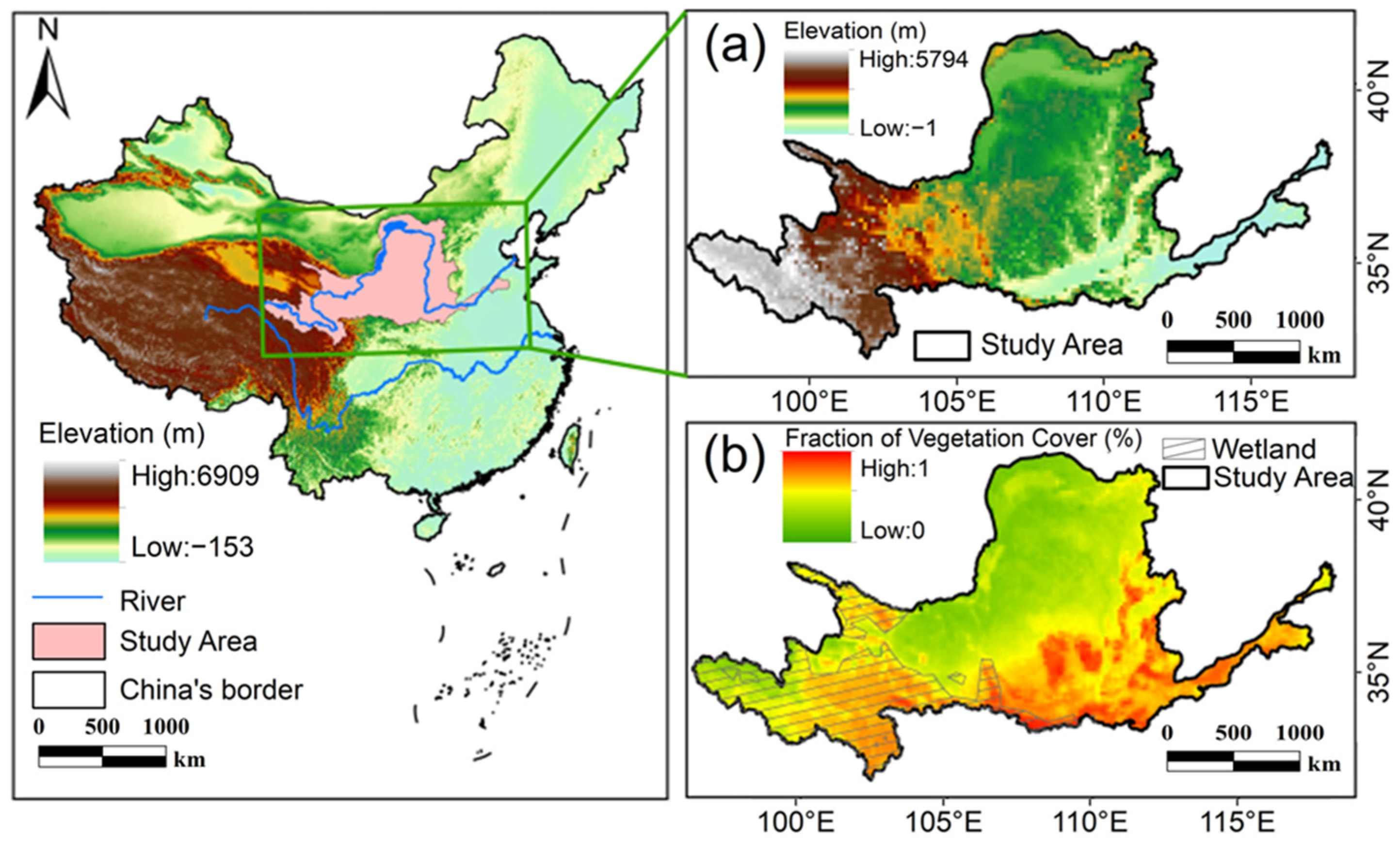
2.1. Study Area

The YRB, spanning from 96° to 119° east longitude and from 32° to 42° north latitude, covers an area of approximately 7.95 × 10⁵ square kilometers. It is the cradle of Chinese civilization and plays a crucial role as an ecological barrier in China [33]. The health of its ecosystem is directly linked to the water security of numerous downstream cities, agricultural production, and regional ecological balance. In recent years, the region’s ecosystem has experienced continuous degradation, and its hydrological functions have declined. The ecological environment and water resources of the basin face a severe crisis, posing a bottleneck to regional ecological protection and high-quality development [31]. Critical issues such as water scarcity, a significant gap in water resources, and the apparent imbalance between supply and demand pose severe threats to the ecological security of the YRB [34]. These challenges restrict the trajectory of high-quality development centered on regional ecology and green growth [35]. Human activities, such as soil conservation measures, increased irrigation demand, and reservoir construction, have significantly impacted the hydrological conditions and vegetation cover in the YRB, altering the distribution of vegetation and the structure of ecosystems within the basin [36].

2.2. Data Sources

This study leverages boundary data from the YRB and its constituent provinces and cities, sourced from the Resource Environment Science and Data Center of the Chinese Academy of Sciences. It employs the United Nations Environment Programme’s aridity criteria, defining arid regions as those where the Aridity Index (AI), the ratio of annual precipitation (P) to potential evapotranspiration (E₀), falls below 0.65, equivalent to an E/P ratio of less than 0.84. Within the YRB, wetlands represent 26.71% of the total land area, in stark contrast to drylands, which constitute 66.14% (Figure 1). This distribution underscores the prevalence of drought and water scarcity across significant portions of the region [37].

In this research, FVC is adopted as the primary indicator of vegetation. The PKU GIMMS Normalized Difference Vegetation Index (NDVI) dataset (PKU GIMMS NDVI, version 1.2) provides uniform global NDVI data spanning from 1982 to 2022 at semi-monthly intervals [38], with a resolution of 1/12°. This dataset is designed to mitigate the prevalent uncertainties in existing studies. Notably, it surpasses its predecessor, GIMMS NDVI3g, in accuracy. Following preprocessing steps, including cropping, gap-filling, projection transformation, and normalization, monthly NDVI data are compiled using the maximum-value composite method for further analysis, facilitating the derivation of necessary FVC metrics. In this study, NDVI data were resampled to a 0.1° × 0.1° resolution to match the spatial resolution of the ERA5-Land dataset, ensuring consistent analysis.

Meteorological data for this study are derived from the publicly available reanalysis dataset of the European Centre for Medium-Range Weather Forecasts’ Fifth Generation (ECMWF), renowned for its comprehensive coverage and high precision. These data, extensively validated and applied by the research community, prove particularly pertinent for the YRB. The study employed data from the ERA5-Land dataset, covering root-zone soil moisture, precipitation, evaporation, and monthly temperatures from 1982 to 2021 (

Table 1. Reanalysis data used in this study.

Variable Name	Short Name	Dimension	Variable Name in Product	Temporal Resolution	Horizontal Resolution
Precipitation	P	3	Total precipitation	Monthly	0.1° × 0.1°
Evapotranspiration	E	3	Evaporation	Monthly	0.1° × 0.1°
2 m temperature	2 mT	3	2 m temperature	Monthly	0.1° × 0.1°
Soil moisture	SM	3	Volumetric soil moisture layer	Monthly	0.1° × 0.1°

). The ERA5-Land dataset encompasses four soil layers (first layer: 0–7 cm; second layer: 7–28 cm; third layer: 28–100 cm; fourth layer: 100–289 cm). This study calculated soil moisture for the 0–100 cm soil layers, based on the proportional distribution across the three soil layers (7:21:72), to effectively represent root-zone soil moisture.

2.3. Research Method

2.3.1. Preprocessing and Calculation of Fractional Vegetation Cover (FVC)

NDVI was derived through a pixel-based binary method [39].

$${NDVI}_i=MAX\left({NDVI}_{jk}\right)$$

(1)

where NDVI_i represents the NDVI value in month i, and NDVI_jk represents the NDVI value in periods j and k of month i. The maximum composite method was employed to mitigate the impacts of clouds, atmospheric conditions, and solar zenith angles, thereby synthesizing NDVI data on a monthly scale for analysis. Subsequently, the FVC was derived from the NDVI calculations.

$$FVC=({NDVI}_i-{NDVI}_{soil})/({NDVI}_{veg}-{NDVI}_{soil})$$

(2)

where FVC is the vegetation coverage, NDVI_soil is the NDVI value of the area that is completely bare soil or without vegetation coverage, and NDVI_veg represents the NDVI value of the pixels that are completely covered by vegetation, that is, the NDVI value of the pure vegetation pixels. According to the interval distribution of NDVI values within the study area, the upper and lower thresholds of NDVI intercepted at the 5% and 95% confidence levels were used as NDVI_soil and NDVI_veg.

2.3.2. Trend Analysis

We used a linear regression based on the least squares method to detect the trend for the annual FVC [40]. The regression coefficient represented the annual FVC change rate:

$$slope(\beta )={\displaystyle \frac{{\sum }_{i=1}^{40}\left({\alpha }_i-\overline{\alpha }\right)\left(y_i-\overline{y}\right)}{{\sum }_{i=1}^{40}{\left({\alpha }_{yi}-\overline{\alpha }\right)}^2}}$$

(3)

where i is the sequential year range (1982–2021), α_i is the annual FVC in the year y_i, and α and $\overline{y}$ are the mean values. Here, slope(β) is the linear slope, the negative slope indicates that β decreases, whereas the positive slope means that β increases. The absolute value of the slope represents the degree of variation in β.

2.3.3. Mann–Kendall Trend Test

The Mann–Kendall method is a simple and intuitive trend detection technique, characterized by its independence from assumptions about data distribution, resilience to outliers, and high sensitivity to time [41]. It is particularly useful in the analysis of time-series data, demonstrating strong regularity and stability. It has been widely applied in trend significance testing for long time-series data. The statistical testing procedure is as follows:

$$S=\sum _{i=1}^{n-1}\sum _{j=i+1}^{n}sgn(x_j-x_i)$$

(4)

$$sgn\left(x_j-x_i\right)=\left\{\begin{array}{c}1,x_j-x_i>0\\ 0,x_j-x_i=0\\ -1,x_j-x_i<0\end{array}\right.$$

(5)

where negative values indicate a decreasing trend, while positive values indicate an increasing trend; x_i and x_j represent the vegetation characteristics data for years i and j (j > i); n is the length of the time series; and S is the MK test statistic and statistical tests are conducted at a significance level of 0.05.

By overlaying the classification results of trend analysis, the Mann–Kendall test yields pixel-scale FVC trend data [8], classified into four types: SUT (significant uptrend), NUT (non-significant uptrend), SDT (significant downtrend), and NDT (non-significant downtrend).

2.3.4. Grey Relational Analysis

Grey relational analysis (GRA) is a method for evaluating the degree of association between factors, based on the similarity of the geometric shapes of sequence curves. The closer the curves, the stronger the correlation between the corresponding sequences [42]. By quantitatively analyzing the development trends in dynamic processes, it compares the statistical data of time series within a system to determine the degree of correlation between the reference sequence and other sequences. A higher correlation indicates closer proximity to the reference sequence. In this study, GRA was conducted by calculating the GRA of long-term time-series dynamics between different meteorological factors, and vegetation coverage was achieved through grey relational degree calculation. The calculation process was as follows:

1. Selection of reference and comparative sequences:

The monthly vegetation coverage was set as the reference sequence, denoted by X = {x(k), i = l, 2,…, n; k = 1, 2, …m}; Phenological parameters were set as the comparative sequence Y = {y(k), i = 1, 2, …, n; k = l, 2, …,m}. Here, X represents the reference sequence, Y represents the comparative sequence, i represents the sequence category number, and k represents the sequence length.

2. Sequence normalization:

To eliminate the dimensional influence, the standardization method was used to normalize the data. The calculation formula was as follows:

$$X_i^{\prime }(k)={\displaystyle \frac{X_i\left(k\right)-\overline{X_i}}{\sigma }}$$

(6)

$$Y_i^{\prime }(k)={\displaystyle \frac{Y_i\left(k\right)-{\bar{Y}}_i}{\sigma }}$$

(7)

3. Maximum difference and minimum difference:

The absolute difference between the comparative sequence and the reference sequence was calculated, where the maximum value is the maximum difference and the minimum value is the minimum difference. The calculation formula was as follows:

$${\mathsf{\Delta }}_i=\left|Y_i^{\prime }\left(k\right)-X_i^{\prime }(k)\right|,i=\mathrm{1,2},\dots ,n;k=\mathrm{1,2},\dots m$$

(8)

4. Grey relational coefficient calculation:

The calculation formula was as follows:

$$\xi (k)={\displaystyle \frac{{min}_i{min}_k{\mathsf{\Delta }}_i\left(k\right)+\alpha \times {max}_i{max}_k{\mathsf{\Delta }}_i\left(k\right)}{{\mathsf{\Delta }}_i\left(k\right)+\alpha \times {max}_i{max}_k{\mathsf{\Delta }}_i\left(k\right)}}$$

(9)

where α is the resolution coefficient. Studies have shown that when α ≤ 0.5463, the resolution is the best. In this study, the resolution coefficient α was set to 0.5 [43].

5. Calculation of average grey relational degree:

The arithmetic mean of all grey relational degrees in the sequence was calculated. The calculation formula was as follows:

$$r_i={\displaystyle \frac{{\sum }_{k=1}^n{\xi }_i\left(k\right)}{n}}$$

(10)

2.3.5. Path Analysis

Path analysis, based on multiple linear regression equations, analyzes the linear relationship between multiple independent variables and a dependent variable. It separates the direct and indirect effects of independent variables on the dependent variable. Compared to geographical detectors, it offers a clearer display of variable relationships in raster data, aiding the analysis of their influence on the dependent variable [44]. By comparing path coefficients’ absolute values, the impact of each independent variable was directly compared. Widely applicable, it performed spatial path analysis to reflect the impact of individual climate differences in variable pairs on FVC at the spatial scale. The calculation formula was as follows:

For an interrelated system, if there is a linear relationship between n independent variables x_i (i = 1, 2, …, n) and a dependent variable y, the regression equation is as follows:

$$y=a_0+a_1{x}_1+a_2{x}_2+\cdots +a_n{x}_n$$

(11)

According to the simple correlation coefficient r_xixj (i, j ≤ n) between the respective variables, and the simple correlation r_xiy (i ≤ n) between the respective variables and the dependent variable, the normal matrix equation can be established through mathematical transformation from Formula (11):

$$\left[\begin{array}{cccc}1& r_{x_1{x}_2}& \cdots & r_{x_1{x}_n}\\ r_{x_2{x}_1}& 1& \cdots & r_{x_2{x}_n}\\ ⋮& ⋮& \ddots & ⋮\\ r_{x_n{x}_1}& r_{x_n{x}_2}& \cdots & 1\end{array}\right]\left[\begin{array}{c}{a}_1\\ a_2\\ ⋮\\ a_n\end{array}\right]=\left[\begin{array}{c}{r}_{x_{1}y}\\ r_{x_{2}y}\\ ⋮\\ r_{x_{n}y}\end{array}\right]$$

(12)

According to Formula (3), the path coefficient a_i can be obtained; ai represents the direct path coefficient of the independent variable xi on the dependent variable y, which is the direct effect of xi on y; r_xixj∙a_i represents the independent variable x_i on the dependent variable through x_j. The indirect path coefficient of y is the indirect effect of x_i on the dependent variable y through x_j.

In order to facilitate the comparison of indicators with different units and magnitudes, all data were first standardized using the Z-score standardization method [45]:

$${\mathrm{X}}_{\mathrm{s}\mathrm{t}\mathrm{d}}={\displaystyle \frac{{\mathrm{X}}_{\mathrm{i}}-\overline{\mathrm{X}}}{\mathsf{\sigma }}}$$

(13)

where x_std is the standardized value, x is the average value of the data sequence x_i, and σ is the corresponding standard deviation.

Multiple linear regression was performed on the standardized FVC, soil moisture (SM), precipitation (P), evapotranspiration (E), and temperature (T):

$$FV{C}_{\mathrm{stad}}=A_{sm}\times SM+A_p\times P+A_e\times E+A_t\times T+\epsilon$$

(14)

where $\epsilon$ is the residual; Asm, Ap, Ae, and At represent the standardized regression coefficient (immediate impact) on FVC, that is, the direct impact of soil moisture, precipitation, evapotranspiration, and temperature on FVC, respectively, without considering the influence of other variables.

Due to the mutual influence between different average climate variables, their interaction was expressed as follows:

$$A_{p,e,t-sm}=r_{p,sm}{\times A}_p+{r_{e,sm}\times A}_e{+r_{t,sm}\times A}_t$$

(15)

$$A_{sm,e,t-p}=r_{sm,p}\times A_{sm}+r_{e,p}\times A_e{+r_{t,p}\times A}_t$$

(16)

$$A_{t,p,sm-e}=r_{t,e}\times A_t+r_{p,e}\times A_p{+r_{sm,e}\times A}_{sm}$$

(17)

$$A_{sm,p,e-t}=r_{sm,t}\times A_{sm}+r_{p,t}\times A_p{+r_{e,t}\times A}_e$$

(18)

where $r_{i,j}$ represents the correlation coefficient between i and j; $A_{p,e,t-sm},A_{sm,e,t-p},A_{t,p,sm-e},{andA}_{sm,p,e-t}$ represent the indirect path coefficients of soil moisture, precipitation, evapotranspiration and temperature on FVC and the indirect effects of soil moisture, precipitation, evapotranspiration and temperature on FVC through other variables, respectively.

According to the principle of path analysis, the correlation coefficient was equal to the sum of the direct path coefficient and the indirect path coefficient, that is, as follows:

$$r_{sm,fvc}=A_{sm}+A_{p,e,t-sm}$$

(19)

$$r_{p,fvc}=A_p+A_{sm,e,t-p}$$

(20)

$$r_{e,fvc}=A_e+A_{t,p,sm-e}$$

(21)

$$r_{t,fvc}=A_t+A_{sm,p,e-t}$$

(22)

where r_sm,fvc, r_p,fvc, r_e,fvc, and r_t,fvc represent the comprehensive effects of soil moisture, precipitation, evapotranspiration, and temperature on FVC, respectively.

2.3.6. Time-Lag and -Accumulation Analysis

The lagged and accumulated climate variables were defined as follows

$$FV{\mathrm{C}}_{t-SM(m,n)}={\displaystyle \frac{1}{n}}{\sum }_{i=0}^n{SM}_{t-m-i}$$

(23)

$$FV{\mathrm{C}}_{t-P(m,n)}={\displaystyle \frac{1}{n}}{\sum }_{i=0}^n{P}_{t-m-i}$$

(24)

$$FV{\mathrm{C}}_{t-E(m,n)}={\displaystyle \frac{1}{n}}{\sum }_{i=0}^n{E}_{t-m-i}$$

(25)

$$FV{\mathrm{C}}_{t-T(m,n)}={\displaystyle \frac{1}{n}}{\sum }_{i=0}^n{T}_{t-m-i}$$

(26)

where m and n range from 0 to 3, and where values of 1 to 3 represent a lag or accumulation times of 1 to 3 months, respectively. Specifically, m represents the number of lagged months, while n represents the number of cumulative months.

The variable $FV{C}_{t-SM(m,n)}$ refers to the FVC at month t with a lag of m months and an accumulation of n months. It was calculated as the average soil moisture (SM) over n months preceding the lagged month. Additionally, ${SM}_{t-m-i}$ represents the ${SM}_{m+i}$ months before the t month.

In this study, the Pearson correlation coefficients were used to assess the linear relationship between FVC and various climatic variables, examining their lagged and cumulative effects on FVC. The correlation coefficients were computed for different combinations of lagged and cumulative months between FVC and each climatic variable. The lag and accumulation months with the highest absolute Pearson correlation coefficients were determined as the lag and accumulation times of climatic variables that significantly influenced FVC [46,47]. These parameters were categorized into 10 classes, labeled as L0A0, L0A1, L0A2, L0A3, L1A0, L1A1, L1A2, L2A0, L2A1, and L3A0, where L_iA_j denotes lagged months i and cumulative months j.

3. Results

3.1. Spatial Pattern and Trends in Meteorological Variables

Figure 2a shows the inter-annual variation in the annual average FVC, revealing a spatial gradient of decreasing vegetation coverage from southeast to northwest. The 18-year YRB average FVC value was 0.4767. The maximum and minimum values appeared in 2018 and 1990, which were 0.6855 and 0.6063, respectively. The 18-year dryland average FVC value was 0.4548. The maximum and minimum values appeared in 2021 and 1985, which were 0.4903 and 0.4256, respectively. The 18-year wetland average FVC value was 0.5614. The maximum and minimum values appeared in 2016 and 2022, which were 0.5859 and 0.5199, respectively. As is shown in Figure 2b the linear change rates of the annual FVC ranged from −0.00076/a to 0.0063/a. Around 51.36% of YRB areas exhibited a positive linear slope in FVC, while approximately 48.64% showed a negative linear trend. Roughly 64.04% of dryland regions demonstrated a positive linear trend in FVC, contrasting with approximately 35.96% displaying a negative linear slope. About 14.24% of wetland territories showcased a positive linear FVC trend, whereas the majority, approximately 85.76%, exhibited a negative linear slope. Across the YRB region, FVC trends varied, with approximately half of the areas displaying a positive linear slope and the other half showing a negative linear trend. However, within specific land types, dryland regions predominantly exhibited a positive linear FVC trend, while wetland areas were largely characterized by a negative linear FVC slope. In terms of the significance of FVC trends, the proportions of vegetated areas with significantly increasing, non-significant, and significantly decreasing FVC trends were 32.78%, 33.21%, and 34.02%, respectively, indicating vegetation restoration in the YRB (Figure 2c). In dryland areas, the proportions of significantly increasing, non-significant, and significantly decreasing FVC trends were 49.49%, 33.81%, and 16.71%, respectively, also suggesting vegetation restoration efforts in this region. Similarly, in wetland areas, the proportions of significantly increasing, non-significant, and significantly decreasing FVC trends were 7.68%, 14.92%, and 77.41%, respectively. This may indicate vegetation loss rather than restoration in this region, requiring further investigation and intervention measures. Analysis revealed distinct variations in land coverage across different categories within the YRB (Figure 2d,

Table 2. FVC classification.

Vegetation Coverage Value	Categories	YRB	Dryland	Wetland
0.00 ≤ FVC < 0.30	Extremely low coverage	21.46%	25.63%	5.44%
0.03 ≤ FVC < 0.45	Low coverage	27.78%	30.37%	18.32%
0.45 ≤ FVC < 0.60	Medium coverage	21.24%	18.74%	31.54%
0.60 ≤ FVC < 0.75	Medium–high coverage	21.93%	16.91%	38.10%
0.75 ≤ FVC < 1.00	High coverage	7.58%	8.34%	6.61%

), focusing on its dryland and wetland regions. In the YRB, high-coverage areas constituted 21.46%, with medium–high-overage areas being slightly higher at 27.78%. Medium-coverage and low-coverage areas accounted for 21.24% and 21.93%, respectively, while extremely-low-coverage areas represented 7.58%. Comparatively, in the dryland regions, medium–high coverage dominated at 30.37%, followed by high coverage at 25.63%. Medium-coverage and low-coverage areas showed proportions of 18.74% and 16.91%, respectively, with extremely-low-coverage areas being slightly higher at 8.34%. Wetland areas exhibited a distinct pattern, with medium coverage being the most prevalent at 31.54%, followed by low coverage at 38.10%. High-coverage areas in wetlands were notably lower at 5.44%. The FVC trends in the provinces of the YRB, and in dryland and wetland areas followed distinct linear patterns over time (Figure 2e). In the YRB, FVC changed annually according to the equation y = 0.00232 × x + −3.73837, while dryland and wetland areas exhibited their unique linear trends described by equations y = 0.00253 × x + −4.08206 and y = 0.00209 × x + −3.36296, respectively. In summary, while the YRB and dryland regions indicated vegetation restoration efforts, the wetland regions suggest potential vegetation loss. Further investigation and intervention measures are necessary to protect and restore wetland vegetation effectively.

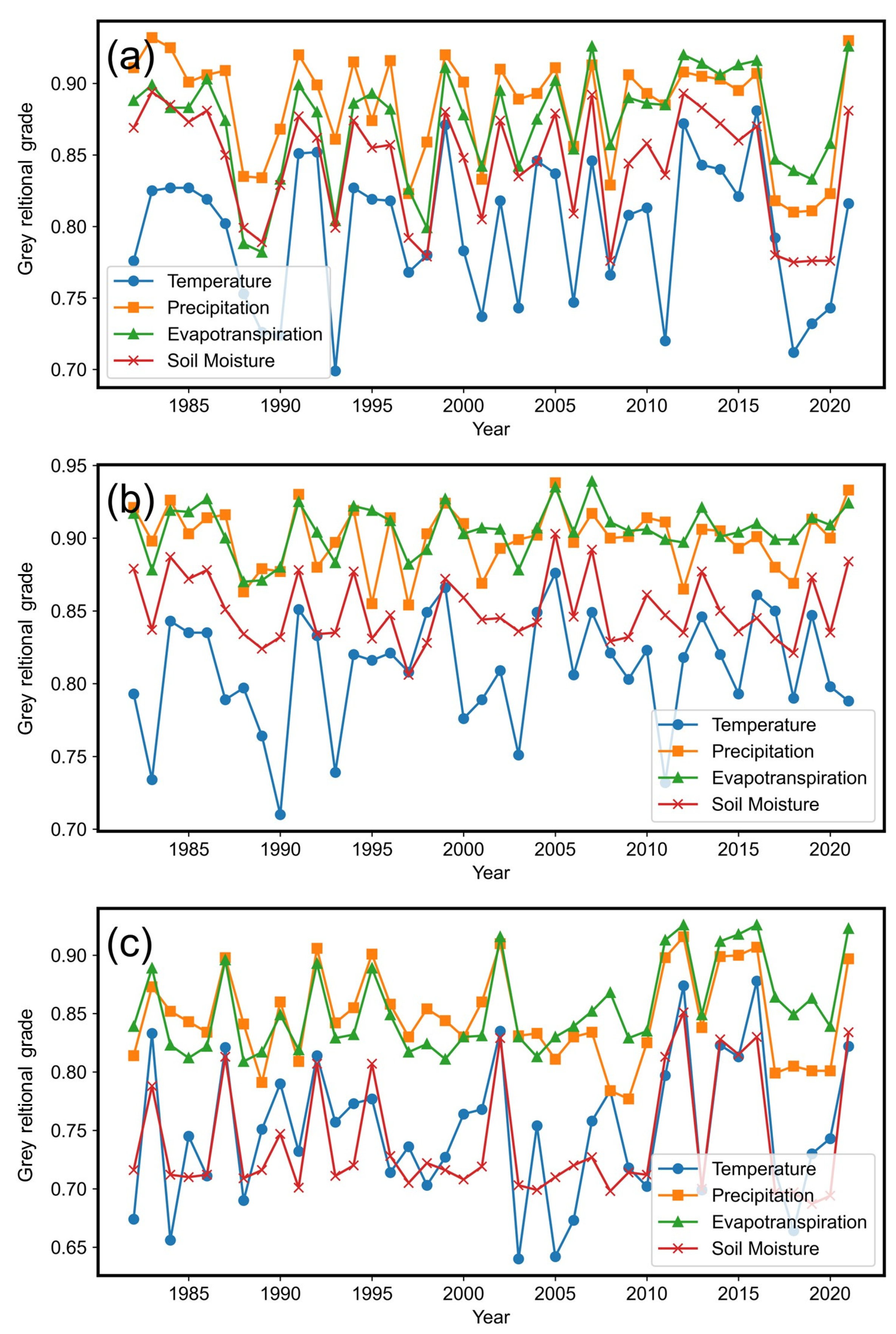
3.2. Grey Relation Analysis

Based on the grey correlation analysis results between each climate element and FVC, the following inferences can be made: as is shown in Figure 3a and

Table A1. Grey relational analysis of FVC with meteorological factors in the YRB.

Year	Temperature	Precipitation	Evapotranspiration	Soil Moisture
1982	0.776	0.911	0.888	0.869
1983	0.825	0.932	0.899	0.894
1984	0.827	0.925	0.883	0.885
1985	0.827	0.901	0.883	0.873
1986	0.819	0.906	0.903	0.881
1987	0.802	0.909	0.874	0.850
1988	0.753	0.835	0.788	0.799
1989	0.726	0.834	0.782	0.789
1990	0.724	0.868	0.833	0.829
1991	0.851	0.920	0.899	0.877
1992	0.852	0.899	0.880	0.862
1993	0.699	0.861	0.804	0.799
1994	0.827	0.915	0.886	0.874
1995	0.819	0.874	0.893	0.855
1996	0.818	0.916	0.882	0.857
1997	0.768	0.823	0.826	0.792
1998	0.780	0.859	0.799	0.779
1999	0.871	0.920	0.911	0.880
2000	0.783	0.901	0.878	0.848
2001	0.737	0.833	0.842	0.805
2002	0.818	0.910	0.895	0.874
2003	0.743	0.889	0.842	0.835
2004	0.846	0.893	0.875	0.845
2005	0.837	0.911	0.902	0.879
2006	0.747	0.856	0.854	0.809
2007	0.846	0.913	0.926	0.892
2008	0.766	0.829	0.857	0.776
2009	0.808	0.887	0.890	0.844
2010	0.813	0.906	0.886	0.858
2011	0.720	0.893	0.885	0.836
2012	0.872	0.908	0.920	0.893
2013	0.843	0.905	0.914	0.883
2014	0.840	0.903	0.906	0.872
2015	0.821	0.895	0.913	0.860
2016	0.881	0.907	0.916	0.870
2017	0.792	0.818	0.847	0.780
2018	0.712	0.810	0.839	0.775
2019	0.732	0.811	0.833	0.776
2020	0.743	0.823	0.858	0.776
2021	0.816	0.930	0.926	0.881
average	0.797	0.883	0.873	0.843
GRA order	4	1	2	3

, in the YRB, the GRAs of the FVC and temperature ranged from 0.699 to 0.881 in the YRB, and the maximum and minimum values appeared in 2016 and 1993; the GRAs of the FVC and precipitation ranged from 0.810 to 0.930 in the YRB, and the maximum and minimum values appeared in 1983 and 2018; the GRAs of the FVC and evapotranspiration ranged from 0.782 to 0.926 in the YRB, and the maximum and minimum values appeared in 2021 and 1989; and the GRAs of the FVC and soil moisture ranged from 0.775 to 0.894 in the YRB, and the maximum and minimum values appeared in 1983 and 2018. Overall, the multi-year average grey correlation degrees between FVC and various meteorological factors in the YRB followed a descending order as follows: GRA_{precipitation} > GRA_{evapotranspiration} > GRA_temperature > GRA_{soil moisture}. As is shown in Figure 3b and

Table A2. Grey relational analysis of FVC with meteorological factors in the dryland areas.

Year	Temperature	Precipitation	Evapotranspiration	Soil Moisture
1982	0.793	0.921	0.917	0.879
1983	0.734	0.898	0.878	0.837
1984	0.843	0.926	0.919	0.887
1985	0.835	0.903	0.918	0.872
1986	0.835	0.914	0.927	0.878
1987	0.789	0.916	0.900	0.851
1988	0.797	0.863	0.870	0.834
1989	0.764	0.879	0.871	0.824
1990	0.710	0.877	0.880	0.832
1991	0.851	0.930	0.925	0.878
1992	0.833	0.880	0.904	0.834
1993	0.739	0.897	0.883	0.835
1994	0.820	0.919	0.922	0.877
1995	0.816	0.855	0.919	0.831
1996	0.821	0.914	0.912	0.847
1997	0.808	0.854	0.882	0.806
1998	0.849	0.903	0.892	0.828
1999	0.866	0.924	0.927	0.872
2000	0.776	0.910	0.903	0.859
2001	0.789	0.869	0.907	0.844
2002	0.809	0.893	0.906	0.845
2003	0.751	0.899	0.878	0.836
2004	0.849	0.902	0.907	0.842
2005	0.876	0.938	0.935	0.903
2006	0.806	0.897	0.904	0.846
2007	0.849	0.917	0.939	0.892
2008	0.821	0.900	0.911	0.829
2009	0.803	0.901	0.905	0.832
2010	0.823	0.914	0.906	0.861
2011	0.732	0.911	0.899	0.847
2012	0.818	0.865	0.897	0.835
2013	0.846	0.906	0.921	0.877
2014	0.820	0.905	0.901	0.850
2015	0.793	0.893	0.904	0.836
2016	0.861	0.901	0.910	0.845
2017	0.850	0.880	0.899	0.831
2018	0.790	0.869	0.899	0.821
2019	0.847	0.913	0.914	0.873
2020	0.798	0.900	0.909	0.835
2021	0.788	0.933	0.924	0.884
average	0.810	0.900	0.906	0.851
GRA order	4	2	1	3

, the GRAs of the FVC and temperature ranged from 0.710 to 0.876 in the dryland areas, and the maximum and minimum values appeared in 2005 and 1990; the GRAs of the FVC and precipitation ranged from 0.854 to 0.938 in the dryland areas, and the maximum and minimum values appeared in 2005 and 1997; the GRAs of the FVC and evapotranspiration ranged from 0.870 to 0.939 in the dryland areas, and the maximum and minimum values appeared in 2007 and 1988; and the GRAs of the FVC and soil moisture ranged from 0.806 to 0.903 in the dryland areas, and the maximum and minimum values appeared in 2005 and 1997. Overall, the multi-year average grey correlation degrees between FVC and various meteorological factors in the dryland areas followed a descending order as follows: GRA_{evapotranspiration} > GRA_{precipitation} > GRA_{soil moisture} > GRA _temperature. As is shown in Figure 3c and

Table A3. Grey relational analysis of FVC with meteorological factors in the wetland areas.

Year	Temperature	Precipitation	Evapotranspiration	Soil Moisture
1982	0.674	0.814	0.839	0.716
1983	0.833	0.873	0.889	0.788
1984	0.656	0.852	0.823	0.712
1985	0.745	0.843	0.812	0.710
1986	0.711	0.834	0.822	0.712
1987	0.821	0.898	0.896	0.813
1988	0.690	0.841	0.809	0.709
1989	0.751	0.791	0.817	0.716
1990	0.790	0.860	0.849	0.747
1991	0.732	0.809	0.819	0.701
1992	0.814	0.906	0.893	0.807
1993	0.757	0.842	0.829	0.711
1994	0.773	0.855	0.832	0.720
1995	0.777	0.901	0.889	0.807
1996	0.714	0.858	0.849	0.728
1997	0.736	0.830	0.817	0.705
1998	0.703	0.854	0.824	0.722
1999	0.727	0.844	0.811	0.716
2000	0.764	0.830	0.830	0.708
2001	0.768	0.860	0.831	0.719
2002	0.835	0.910	0.916	0.829
2003	0.640	0.831	0.830	0.703
2004	0.754	0.833	0.813	0.699
2005	0.642	0.811	0.830	0.710
2006	0.673	0.830	0.839	0.720
2007	0.758	0.834	0.852	0.727
2008	0.784	0.784	0.868	0.698
2009	0.718	0.777	0.829	0.714
2010	0.702	0.825	0.835	0.712
2011	0.797	0.898	0.913	0.813
2012	0.874	0.916	0.926	0.851
2013	0.699	0.838	0.849	0.700
2014	0.823	0.899	0.912	0.828
2015	0.813	0.900	0.918	0.815
2016	0.878	0.907	0.926	0.830
2017	0.715	0.799	0.864	0.697
2018	0.664	0.805	0.849	0.697
2019	0.730	0.801	0.863	0.687
2020	0.743	0.801	0.839	0.694
2021	0.822	0.897	0.923	0.834
average	0.750	0.847	0.854	0.741
GRA order	3	2	1	4

, the GRAs of the FVC and temperature ranged from 0.640 to 0.878 in the wetland areas, and the maximum and minimum values appeared in 2016 and 2003; the GRAs of the FVC and precipitation ranged from 0.777 to 0.916 in the wetland areas, and the maximum and minimum values appeared in 2012 and 2009; the GRAs of the FVC and evapotranspiration ranged from 0.809 to 0.926 in the wetland areas, and the maximum and minimum values appeared in 2012 and 1988; and the GRAs of the FVC and soil moisture ranged from 0.687 to 0.851 in the wetland areas, and the maximum and minimum values appeared in 2012 and 2019. Overall, the multi-year average grey correlation degrees between FVC and various meteorological factors in the wetland areas followed a descending order as follows: GRA_{evapotranspiration} > GRA_{precipitation} > GRA_temperature > GRA_{soil moisture}.

Taking into account the utilization of grey relational analysis to investigate the annual variations in meteorological elements on FVC in the YRB, irrespective of whether in the wetland or dryland regions, the spatial heterogeneity was evident in the influence of these elements on FVC. However, precipitation and evapotranspiration were relatively dominant factors, while soil moisture and temperature were secondary. This phenomenon likely stemmed from the geographical and climatic characteristics of the YRB, where much of the region experienced a semi-arid to semi-humid climate, with vegetation growth primarily constrained by water availability. Consequently, fluctuations in precipitation directly impact soil moisture and vegetation water supply, thereby determining the vegetation’s consumption rate of soil moisture. Conversely, evapotranspiration reflects vegetation’s demand for and utilization of water, thus playing a crucial role in the hydrological cycle and directly influencing vegetation growth and distribution. Considering hydrological cycles, the water supply–demand balance, and climate factors collectively, precipitation and evapotranspiration played a predominant role in the vegetation cover of the YRB, with soil moisture and temperature exerting relatively minor effects. Specifically, soil moisture exhibited a certain lag effect, influenced by precipitation, but its effects typically did not manifest immediately, rather exhibiting a certain lag period. Similarly, temperature’s impact on vegetation growth and metabolic activities also exhibited a lag. Temperature fluctuations affect the growth rate and transpiration of plants, yet plant responses to temperature generally entail a time delay. Moreover, the diverse topography, soil types, and vegetation in the YRB may result in spatial variations in the impact of meteorological elements on FVC.

3.3. Path Analysis of Meteorological Factors and FVC in Spatial and Temporal Dimensions

According to Figure 4 and

Table 3. Path analysis statistical data in the YRB.

Category	Values	Soil Moisture	Precipitation	Evapotranspiration	Temperature
Immediate impacts (II)	Min	−0.372	−0.513	−0.407	−0.151
	Mean	0.401	0.204	0.075	0.003
	Max	0.981	0.616	0.585	0.133
	STD	0.202	0.176	0.151	0.026
Indirect impacts (DI)	Min	−0.380	−0.103	−0.251	−0.107
	Mean	0.217	−0.001	0.145	−0.003
	Max	0.724	0.074	0.794	0.099
	STD	0.150	0.019	0.206	0.025
Combined impacts (CI)	Min	−0.312	−0.522	−0.390	−0.154
	Mean	0.617	0.204	0.220	0.000
	Max	1.044	0.628	0.899	0.141
	STD	0.192	0.175	0.282	0.036
	Min	−0.312	−0.522	−0.390	−0.154

,

Table 4. Path analysis statistical data in the dryland areas.

Category	Values	Soil Moisture	Precipitation	Evapotranspiration	Temperature
Immediate impacts (II)	Min	−0.372	−0.513	−0.407	−0.151
	Mean	0.401	0.204	0.075	0.003
	Max	0.981	0.616	0.585	0.133
	STD	0.202	0.176	0.151	0.026
Indirect impacts (DI)	Min	−0.380	−0.103	−0.251	−0.107
	Mean	0.217	−0.001	0.145	−0.003
	Max	0.724	0.074	0.794	0.099
	STD	0.150	0.019	0.206	0.025
Combined impacts (CI)	Min	−0.312	−0.522	−0.390	−0.154
	Mean	0.617	0.204	0.220	0.000
	Max	1.044	0.628	0.899	0.141
	STD	0.192	0.175	0.282	0.036
	Min	−0.312	−0.522	−0.390	−0.154

and

Table 5. Path analysis statistical data in the wetland areas.

Category	Values	Soil Moisture	Precipitation	Evapotranspiration	Temperature
Immediate impacts (II)	Min	−0.372	−0.513	−0.407	−0.151
	Mean	0.401	0.204	0.075	0.003
	Max	0.981	0.616	0.585	0.133
	STD	0.202	0.176	0.151	0.026
Indirect impacts (DI)	Min	−0.380	−0.103	−0.251	−0.107
	Mean	0.217	−0.001	0.145	−0.003
	Max	0.724	0.074	0.794	0.099
	STD	0.150	0.019	0.206	0.025
Combined impacts (CI)	Min	−0.312	−0.522	−0.390	−0.154
	Mean	0.617	0.204	0.220	0.000
	Max	1.044	0.628	0.899	0.141
	STD	0.192	0.175	0.282	0.036
	Min	−0.312	−0.522	−0.390	−0.154

, the path analysis results provided insights into the extent and spatial distribution characteristics of various climatic variables affecting FVC in different regions of the YRB. Figure 4a,e,i illustrate the impact of soil moisture on FVC, showing a significant direct influence of soil moisture on FVC in dryland areas, with immediate impacts (II) = 0.401. This could be attributed to the limited vegetation growth in dryland areas, where increased soil moisture facilitated the provision of necessary water for growth. In contrast, in wetland areas, the direct impact of soil moisture on FVC was relatively minor (II = 0.138), likely due to the inherently higher soil moisture content in wetlands, resulting in fewer constraints on vegetation growth. Considering both direct and indirect effects, soil moisture exhibited a higher comprehensive impact on FVC, with combined impacts (CI) = 0.617.

Figure 4b,f,j depict the influence of precipitation on FVC, indicating a relatively stable direct impact of precipitation on FVC in both dryland and wetland regions of the YRB (II dryland = 0.204, II wetland = 0.219). This suggested that precipitation provided essential moisture and nutrients for vegetation growth. However, the indirect impact (DI) of precipitation on FVC was slightly higher in wetland compared to dryland regions (DI wetland = 0.019, DI dryland = −0.001). Considering both direct and indirect effects, the comprehensive impact of precipitation on FVC differed between dryland and wetland regions (CI dryland = 0.204, CI wetland = 0.178), possibly due to differences in the interaction between precipitation and soil moisture in different ecosystems.

Figure 4c,g,k illustrate the effect of evapotranspiration on FVC, showing a lower direct impact of evapotranspiration on FVC in dryland areas a(II dryland = 0.075), while the direct impact significantly increased in wetland areas (II wetland = 0.343). This could be attributed to the higher evapotranspiration rate in wetlands, leading to increased water demand for vegetation, thereby exacerbating the direct impact of evapotranspiration on FVC. The indirect impact of evapotranspiration on FVC was slightly higher in wetland than in dryland areas (DI wetland = 0.252, DI dryland = 0.145). Considering both direct and indirect effects, the comprehensive impact of evapotranspiration on FVC was significantly higher in wetland than in dryland areas (CI wetland = 0.823, CI dryland = 0.220), indicating that wetland vegetation is more susceptible to the influence of evapotranspiration.

Figure 4d,h,l demonstrate the impact of temperature on FVC, with a relatively small direct effect of temperature on FVC, close to zero, consistent with the results of the grey relational analysis (II dryland = 0.003, II wetland = 0.009). The indirect impact of temperature on FVC was slightly higher in wetland than in dryland areas (DI wetland = 0.021, DI dryland = −0.003). Considering both direct and indirect effects, the comprehensive impact of temperature on FVC was slightly higher in wetland than in dryland areas (CI wetland = 0.030, CI dryland = 0), possibly due to the higher sensitivity of wetland vegetation to temperature.

In summary, regarding direct effects, evapotranspiration exhibited the most significant influence, with an average value of 0.401, ranging from a minimum of −0.372 to a maximum of 0.981, indicating its significant and widespread impact on the dependent variable. Next was precipitation, with an average value of 0.204, ranging from a minimum of −0.513 to a maximum of 0.616, demonstrating its importance. In contrast, the direct impacts of soil moisture and temperature were relatively minor, characterized by smaller fluctuations and lower average values, with the range of soil moisture impact ranging from −0.407 to 0.585 with an average value of 0.075, and the range of temperature impact ranging from −0.151 to 0.133 with an average value of 0.003. This result was consistent with the results of previous grey relational analysis, indicating that precipitation and evapotranspiration relatively dominated, while soil moisture and temperature were secondary factors. In terms of indirect effects, both evapotranspiration and soil moisture played prominent roles, particularly with soil moisture exerting a more significant indirect impact on FVC, highlighting its importance in the causal pathway. The comprehensive impact results indicated that evapotranspiration remained the dominant factor, but the combined effects of soil moisture and precipitation should not be overlooked. Conversely, temperature played a relatively minor role in the overall impact, with its influence being small and relatively stable.

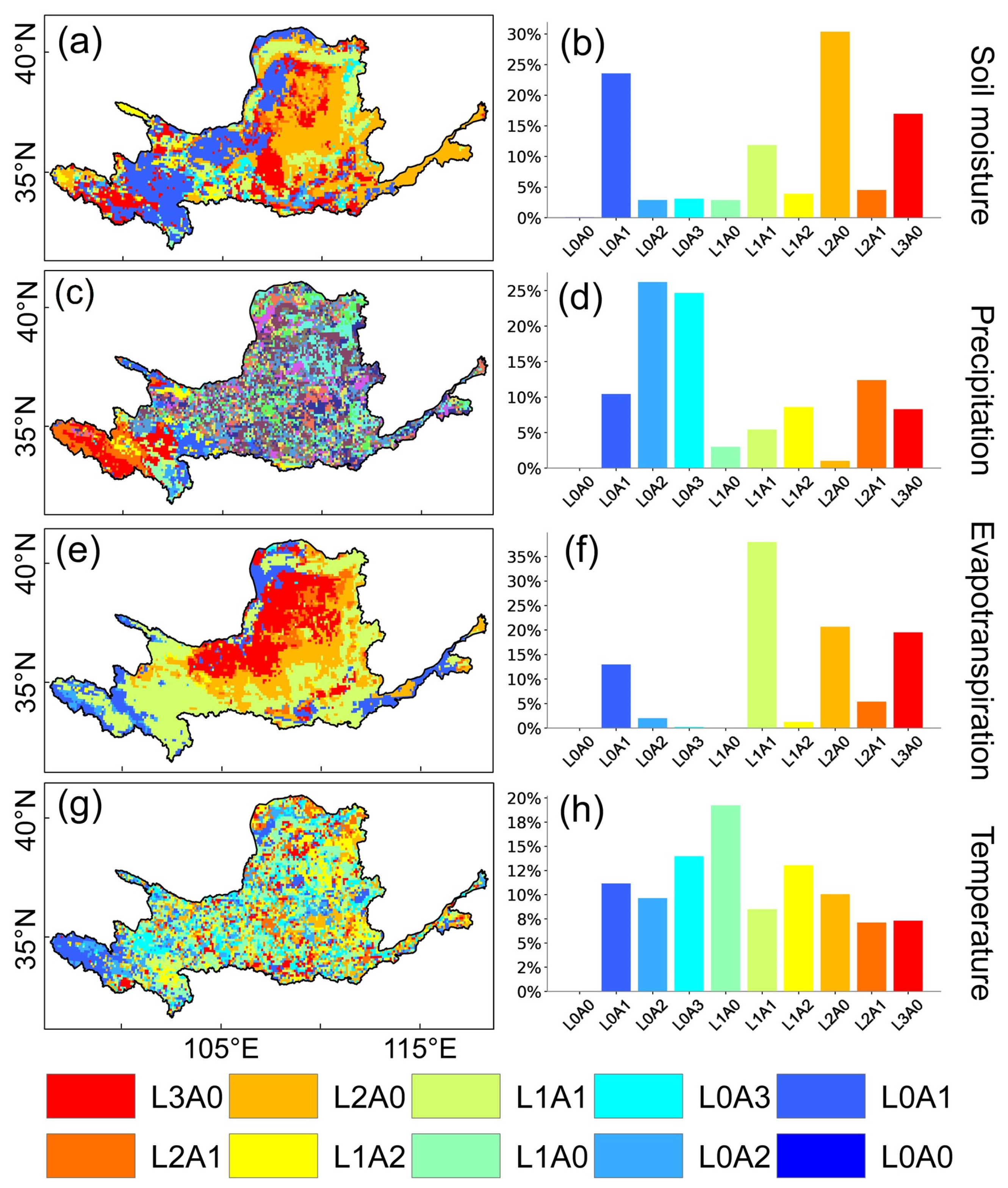
3.4. The Time-Lag and -Accumulation Effects of Meteorological Factors on FVC Changes

The impact of various meteorological factors on vegetation exhibits time-lag and time-accumulation effects. Analyzing the cumulative time and area proportions of meteorological factors, including soil moisture, precipitation, evaporation, and temperature, over 0–3 months in different regions (dryland and wetland) of the YRB enables the quantification of their effects on vegetation (Figure 5).

We examined the temporal accumulation of various meteorological elements across the entire YRB, encompassing its total area as well as its arid and humid regions (

Table 6. Time-lag and -accumulation analysis statistical data in the YRB.

Category	Soil Moisture	Precipitation	Evapotranspiration	Temperature
L0A0	0.05	0.02	0.02	0.02
L0A1	23.57	10.42	12.96	11.16
L0A2	2.88	26.20	2.00	9.63
L0A3	3.09	24.67	0.20	13.96
L1A0	2.87	2.98	0.05	19.23
L1A1	11.84	5.43	37.96	8.49
L1A2	3.88	8.60	1.25	13.05
L2A0	30.37	1.00	20.66	10.04
L2A1	4.51	12.38	5.37	7.10
L3A0	16.95	8.29	19.54	7.31

). Within the YRB, soil moisture exhibited a lag of 1.392 months with an accumulation period of 0.627 months. The predominant combinations of lag and accumulation for soil moisture were denoted as L0A1 and L2A0, constituting 23.57% and 30.37% of the total area, respectively. Precipitation experienced a lag of 0.686 months with an accumulation of 1.718 months, with the primary combinations being L0A2 and L0A3, accounting for 26.2% and 24.67% of the total area, respectively. Evapotranspiration displayed a lag of 1.499 months and an accumulation of 0.634 months, with the primary combinations identified as L1A1 and L2A0, covering 37.96% and 20.66% of the total area, respectively. Temperature demonstrated a lag of 0.970 months and an accumulation of 1.140 months, with the primary combinations designated as L0A3 and L1A0, representing 13.96% and 19.23% of the total area, respectively.

Within the drylands (

Table 7. Time-lag and -accumulation analysis statistical data in the dryland regions.

Category	Soil Moisture	Precipitation	Evapotranspiration	Temperature
L0A0	0.05	0.02	0.02	0.02
L0A1	18.35	7.53	10.44	7.35
L0A2	2.82	32.24	0.14	8.54
L0A3	3.40	31.15	0.24	14.91
L1A0	2.07	1.48	0.06	20.54
L1A1	13.68	5.46	29.23	6.59
L1A2	2.13	7.75	1.53	14.61
L2A0	36.90	1.23	26.38	10.68
L2A1	5.47	9.90	6.83	8.70
L3A0	15.13	3.26	25.14	8.07

), soil moisture exhibited a lag of 1.480 months with an accumulation of 0.576 months. The dominant combinations for soil moisture were noted as L0A1 and L2A0, comprising 18.35% and 36.9% of the total area, respectively. Precipitation showed a lag of 0.467 months with an accumulation of 1.963 months, with the primary combinations being L0A2 and L0A3, accounting for 32.24% and 31.15% of the total area, respectively. Evapotranspiration demonstrated a lag of 1.727 months and an accumulation of 0.506 months, with the primary combinations identified as L1A1 and L2A0, covering 29.23% and 26.38% of the total area, respectively. Temperature displayed a lag of 1.047 months and an accumulation of 1.137 months, with the primary combinations designated as L1A1 and L2A0, representing 14.91% and 20.54% of the total area, respectively.

In the wetlands (

Table 8. Time-lag and -accumulation analysis statistical data in the wetland regions.

Category	Soil Moisture	Precipitation	Evapotranspiration	Temperature
L0A0	0.05	0.05	0.05	0.05
L0A1	41.03	20.12	21.39	23.88
L0A2	3.09	6.01	8.20	13.24
L0A3	2.02	2.98	0.05	10.80
L1A0	5.53	7.98	0.00	14.84
L1A1	5.69	5.32	67.16	14.84
L1A2	9.74	11.44	0.32	7.82
L2A0	8.52	0.27	1.54	7.93
L2A1	1.28	20.70	0.48	1.76
L3A0	23.04	25.12	0.80	4.79

), soil moisture lagged by 1.097 months with an accumulation of 0.797 months. The primary combinations for soil moisture were denoted as L0A1 and L3A0, accounting for 41.03% and 23.04% of the total area, respectively. Precipitation demonstrated a lag of 1.430 months with an accumulation of 0.900 months, with the predominant combinations being L2A1 and L3A0, covering 20.7% and 25.12% of the total area, respectively. Evapotranspiration exhibited a lag of 0.739 months and an accumulation of 1.062 months, with the primary combinations identified as L0A1 and L1A1, comprising 21.39% and 67.16% of the total area, respectively. Temperature showed a lag of 0.713 months and an accumulation of 1.150 months, with the predominant combination noted as L0A1, representing 23.88% of the total area.

Based on the accumulated time–area proportion data of meteorological elements in different regions of the YRB, notable differences existed in the temporal accumulation distribution of precipitation, evapotranspiration, and other factors among these regions. These disparities had significant implications for vegetation growth and ecosystem stability. In dryland regions, the maximum precipitation accumulation value reached 1.963 months, indicating that precipitation accumulated rapidly in the short term. However, with a lag time of only 0.467 months, such accumulation dissipated quickly [48,49]. In contrast, soil moisture in these regions had a lower maximum accumulation value of 0.576 months and a longer lag time of 1.480 months, suggesting that while water retention in the soil was prolonged, accumulation occurred at a slower pace [50]. Wetland regions presented a different scenario, where the maximum soil moisture accumulation value was 0.797 months, with a lag time of 1.097 months, indicating a relatively better water retention capability. The maximum precipitation accumulation value in wetlands was 0.900 months with a lag time of 1.430 months, reflecting a slower but more stable water accumulation, which reduced the likelihood of rapid evaporation [51]. Soil moisture exhibited a greater cumulative effect on FVC in dryland regions, while in wetland regions, it showed more lagged effects on FVC. In dryland regions, due to the scarcity of soil moisture, vegetation growth relies more on soil moisture, leading to its gradual accumulation and hence cumulative effects. Conversely, in wetland regions, where soil moisture was abundant, FVC responded more rapidly to precipitation, demonstrating lagged effects. In dryland regions, the storage of soil moisture took time, leading to lagged effects of precipitation on FVC; whereas in wetland regions, where soil moisture was plentiful, FVC responded more quickly to precipitation, resulting in cumulative effects. These quantified data revealed fundamental differences in water cycling and retention between dryland and wetland regions.

4. Discussion

This study’s examination of vegetation changes in the YRB over the past 40 years reveals a complex interplay between ecological dynamics and human interventions. We observed that while wetlands showed a decrease in FVC, dryland areas experienced an increase, reflecting the substantial impact of conservation initiatives like the Grain for Green Program (GGP) [52,53]. These trends suggest a broader ecological phenomenon where human activity, including reforestation and improved agricultural practices, directly influences vegetation recovery in targeted areas, consistent with ecological theories on human–nature interactions [54,55]. Despite the robust methods employed, such as slope analysis and the Mann–Kendall test, this study faces inherent uncertainties primarily associated with the use of FVC as an indicator of vegetation health. The reliability of FVC can be compromised by the mixed pixel problem in remote sensing data, potentially obscuring finer details of vegetation dynamics [56,57,58]. Resampling, used to adjust the resolution or pixel arrangement of spatial raster data, is a common practice in resolution adjustment, geometric correction, image fusion, and multi-temporal analysis. However, this process may result in the loss of spatial heterogeneity information. Additionally, while GRA provides a comprehensive assessment of the influences on FVC, it does not establish causality, limiting the definitiveness of our conclusions regarding the direct impacts of climatic variables. Our findings on the effects of climatic variables on FVC align with and diverge from existing studies. Like research that has isolated the impacts of individual climate factors on vegetation [59,60,61], our use of GRA and path analysis offers a deeper insight into how these factors interact and collectively affect vegetation, a method not typically employed in conventional studies. This approach has revealed that interactions between soil moisture, air temperature, precipitation, and evapotranspiration add layers of complexity to vegetation dynamics [62,63,64,65,66], highlighting significant regional variations in vegetation response, similar to findings in other global regions where increased precipitation intensity has boosted vegetation growth [67,68]. While the study advances understanding of vegetation dynamics in the YRB, it also reveals inadequacies, such as the potential oversimplification of complex ecological processes by not accounting for below-ground biomass and other non-visible aspects of ecosystem health. Future research should delve deeper into the spatial variability of these relationships by focusing on smaller study areas, such as protected areas, and integrating detailed vegetation characteristics with fine coverage data to fully capture ecosystem dynamics. Innovatively, this research integrates path analysis to parse the direct and indirect effects of multiple interacting climatic variables on vegetation growth [56,69], representing a significant methodological enhancement over traditional statistical models. This novel application provides a more nuanced understanding of the ecological impacts of climate change and human management practices, offering valuable insights for future ecological modeling and conservation strategies [70]. These insights are critical for developing targeted measures to protect and restore the diverse ecological landscapes of the YRB.

5. Conclusions

Climate change significantly impacts terrestrial vegetation growth, and cumulative climate effects are crucial for understanding vegetation dynamics [71,72,73,74]. In this study, we investigated the spatiotemporal dynamics of the FVC across the YRB from 1982 to 2021, examining the impacts of meteorological factors (temperature, precipitation, soil moisture, and evapotranspiration) on FVC through grey relational analysis, path analysis, and time-lag and -accumulation effects analysis. Our findings highlight divergent vegetation dynamics between drylands and wetlands in the YRB. Drylands have shown significant vegetation recovery, with an average FVC of 0.4548 and 49.49% showing a notable increase, while wetlands, despite an average FVC of 0.5614, have experienced significant declines in 77.41% of the areas. Precipitation and evapotranspiration emerged as the primary drivers of FVC changes in both regions, with soil moisture and temperature exerting less impact. Path analysis supports the dominant role of evapotranspiration in directly influencing FVC, complemented by significant indirect effects from soil moisture. The quick accumulation and rapid loss of precipitation in drylands versus better water retention in wetlands suggest tailored management strategies are necessary to address specific climatic impacts on these ecosystems. In future investigations of vegetation–climate interactions, it is essential to integrate the cumulative and lag effects of various climate factors into terrestrial ecosystem models.

References

1. Hill, M.J.; Guerschman, J.P. The MODIS global vegetation fractional cover product 2001–2018: Characteristics of vegetation fractional cover in grasslands and savanna woodlands. Remote Sens. 2020, 12, 406. [Google Scholar] [CrossRef]
2. Huang, C.; Huang, X.; Peng, C.; Zhou, Z.; Teng, M.; Wang, P. Land use/cover change in the Three Gorges Reservoir area, China: Reconciling the land use conflicts between development and protection. Catena 2019, 175, 388–399. [Google Scholar] [CrossRef]
3. Liu, H.; Li, X.; Mao, F.; Zhang, M.; Zhu, D.; He, S.; Huang, Z.; Du, H. Spatiotemporal evolution of fractional vegetation cover and its response to climate change based on MODIS data in the subtropical region of China. Remote Sens. 2021, 13, 913. [Google Scholar] [CrossRef]
4. Agele, S.; Adejobi, K.; Charles, F.; Ogunleye, A.; Olayemi, L. Impacts and feedbacks of land use and land cover patterns in landscapes on ecosystem processes and microclimate: Case of a cacao-based agroforestry landscape. Curr. J. Appl. Sci. Technol. 2017, 22, 1–11. [Google Scholar]
5. Filipponi, F.; Valentini, E.; Nguyen Xuan, A.; Guerra, C.A.; Wolf, F.; Andrzejak, M.; Taramelli, A. Global MODIS fraction of green vegetation cover for monitoring abrupt and gradual vegetation changes. Remote Sens. 2018, 10, 653. [Google Scholar] [CrossRef]
6. Huang, S.; Zheng, X.; Ma, L.; Wang, H.; Huang, Q.; Leng, G.; Meng, E.; Guo, Y. Quantitative contribution of climate change and human activities to vegetation cover variations based on GA-SVM model. J. Hydrol. 2020, 584, 124687. [Google Scholar] [CrossRef]
7. Kaye, J.P.; Quemada, M.J. Using cover crops to mitigate and adapt to climate change. A review. Agron. Sustain. Dev. 2017, 37, 4. [Google Scholar] [CrossRef]
8. Wu, D.; Wu, H.; Zhao, X.; Zhou, T.; Tang, B.; Zhao, W.; Jia, K. Evaluation of spatiotemporal variations of global fractional vegetation cover based on GIMMS NDVI data from 1982 to 2011. Remote Sens. 2014, 6, 4217–4239. [Google Scholar] [CrossRef]
9. Tang, L.; He, M.; Li, X. Verification of fractional vegetation coverage and NDVI of desert vegetation via UAVRS technology. Remote Sens. 2020, 12, 1742. [Google Scholar] [CrossRef]
10. Wan, L.; Zhu, J.; Du, X.; Zhang, J.; Han, X.; Zhou, W.; Li, X.; Liu, J.; Liang, F.; He, Y.; et al. A model for phenotyping crop fractional vegetation cover using imagery from unmanned aerial vehicles. J. Exp. Bot. 2021, 72, 4691–4707. [Google Scholar] [CrossRef]
11. Zhang, J.; Zhang, Z.; Chen, J.; Chen, H.; Jin, J.; Han, J.; Wang, X.; Song, Z.; Wei, G. Development. Estimating soil salinity with different fractional vegetation cover using remote sensing. Land Degrad. Dev. 2021, 32, 597–612. [Google Scholar] [CrossRef]
12. Wang, Y.; Liu, B.; Zhao, J.; Ye, C.; Wei, L.; Sun, J.; Chu, C.; Ming Lee, T. Global patterns and abiotic drivers of ecosystem multifunctionality in dominant natural ecosystems. Environ. Int. 2022, 168, 107480. [Google Scholar] [CrossRef]
13. Han, H.; Yin, Y.; Zhao, Y.; Qin, F. Spatiotemporal Variations in Fractional Vegetation Cover and Their Responses to Climatic Changes on the Qinghai–Tibet Plateau. Remote Sens. 2023, 15, 2662. [Google Scholar] [CrossRef]
14. Li, P.; He, Z.; He, D.; Xue, D.; Wang, Y.; Cao, S. Fractional vegetation coverage response to climatic factors based on grey relational analysis during the 2000–2017 growing season in Sichuan Province, China. Int. J. Remote Sens. 2020, 41, 1170–1190. [Google Scholar] [CrossRef]
15. Zhuang, Q.; Wu, S.; Feng, X.; Niu, Y. Analysis and prediction of vegetation dynamics under the background of climate change in Xinjiang, China. PeerJ 2020, 8, e8282. [Google Scholar] [CrossRef] [PubMed]
16. Liu, T.; Zhang, Q.; Li, T.; Zhang, K. Dynamic Vegetation Responses to Climate and Land Use Changes over the Inner Mongolia Reach of the Yellow River Basin, China. Remote Sens. 2023, 15, 3531. [Google Scholar] [CrossRef]
17. Zhu, X.; He, H.S.; Zhang, S.; Dijak, W.D.; Fu, Y. Interactive effects of climatic factors on seasonal vegetation dynamics in the Central Loess Plateau, China. Forests 2019, 10, 1071. [Google Scholar] [CrossRef]
18. Knapp, A.K.; Ciais, P.; Smith, M.D. Reconciling inconsistencies in precipitation–productivity relationships: Implications for climate change. New Phytologist 2017, 214, 41–47. [Google Scholar] [CrossRef]
19. Yongyong, Z.; Jinjin, H.; Guoxia, M.; Xiaoyan, Z.; Aifeng, L.; Wei, W.; Zhonggen, W. Regional differences of water regulation services of terrestrial ecosystem in the Tibetan Plateau: Insights from multiple land covers. J. Clean. Prod. 2021, 283, 125216. [Google Scholar] [CrossRef]
20. Maia, A.G.; Miyamoto, B.C.B.; Garcia, J.R. Climate change and agriculture: Do environmental preservation and ecosystem services matter? Ecol. Econ. 2018, 152, 27–39. [Google Scholar] [CrossRef]
21. Mo, X.-G.; Hu, S.; Lin, Z.-H.; Liu, S.-X.; Xia, J. Impacts of climate change on agricultural water resources and adaptation on the North China Plain. Adv. Clim. Chang. Res. 2017, 8, 93–98. [Google Scholar] [CrossRef]
22. Zeng, Y.; Yang, X.; Fang, N.; Shi, Z. Large-scale afforestation significantly increases permanent surface water in China’s vegetation restoration regions. Agric. For. Meteorol. 2020, 290, 108001. [Google Scholar] [CrossRef]
23. Wang, J.; Wang, K.; Zhang, M.; Zhang, C. Impacts of climate change and human activities on vegetation cover in hilly southern China. Ecol. Eng. 2015, 81, 451–461. [Google Scholar] [CrossRef]
24. Li, L.; Zha, Y.; Zhang, J.; Li, Y.; Lyu, H. Effect of terrestrial vegetation growth on climate change in China. J. Environ. Manag. 2020, 262, 110321. [Google Scholar] [CrossRef]
25. Li, L.; Zhu, L.; Xu, N.; Liang, Y.; Zhang, Z.; Liu, J.; Li, X. Climate Change and Diurnal Warming: Impacts on the Growth of Different Vegetation Types in the North–South Transition Zone of China. Land 2022, 12, 13. [Google Scholar] [CrossRef]
26. Running, S.W.; Nemani, R.R.; Heinsch, F.A.; Zhao, M.; Reeves, M.; Hashimoto, H. A continuous satellite-derived measure of global terrestrial primary production. Bioscience 2004, 54, 547–560. [Google Scholar] [CrossRef]
27. de Jong, R.; Schaepman, M.E.; Furrer, R.; De Bruin, S.; Verburg, P.H. Spatial relationship between climatologies and changes in global vegetation activity. Glob. Chang. Biol. 2013, 19, 1953–1964. [Google Scholar] [CrossRef] [PubMed]
28. Ma, Y.; Guan, Q.; Sun, Y.; Zhang, J.; Yang, L.; Yang, E.; Li, H.; Du, Q. Three-dimensional dynamic characteristics of vegetation and its response to climatic factors in the Qilian Mountains. Catena 2022, 208, 105694. [Google Scholar] [CrossRef]
29. Zhu, J.; Zeng, X.; Zhang, M.; Dai, Y.; Ji, D.; Li, F.; Zhang, Q.; Zhang, H.; Song, X. Evaluation of the new dynamic global vegetation model in CAS-ESM. Adv. Atmos. Sci. 2018, 35, 659–670. [Google Scholar] [CrossRef]
30. Sa, R.; Yin, S.; Bao, Y.; Bao, H. Change of Desertification based on MODIS Data in the Mongolia Border Region. In Proceedings of the 7th Annual Meeting of Risk Analysis Council of China Association for Disaster Prevention (RAC-2016), Changsha, China, 4–6 November 2016; pp. 837–843. [Google Scholar]
31. Zhang, Q.; Wang, G.; Yuan, R.; Singh, V.P.; Wu, W.; Wang, D. Dynamic responses of ecological vulnerability to land cover shifts over the Yellow River Basin, China. Ecol. Indic. 2022, 144, 109554. [Google Scholar] [CrossRef]
32. Zhang, Q.; Liu, J.; Singh, V.P.; Shi, P.; Sun, P. Hydrological responses to climatic changes in the Yellow River basin, China: Climatic elasticity and streamflow prediction. J. Hydrol. 2017, 554, 635–645. [Google Scholar] [CrossRef]
33. Li, T.; Zhang, Q.; Singh, V.P.; Zhao, J.; Song, J.; Sun, S.; Wang, G.; Shen, Z.; Wu, W. Identification of degradation areas of ecological environment and degradation intensity assessment in the Yellow River Basin. Front. Earth Sci. 2022, 10, 922013. [Google Scholar] [CrossRef]
34. Feng, Y.; Zhu, A.; Liu, P.; Liu, Z. Coupling and coordinated relationship of water utilization, industrial development and ecological welfare in the Yellow River Basin, China. J. Clean. Prod. 2022, 379, 134824. [Google Scholar] [CrossRef]
35. Yang, T.; Zhang, Q.; Chen, Y.D.; Tao, X.; Xu, C.y.; Chen, X. A spatial assessment of hydrologic alteration caused by dam construction in the middle and lower Yellow River, China. Hydrol. Process. Int. J. 2008, 22, 3829–3843. [Google Scholar] [CrossRef]
36. Yang, Y.; Tian, F. Abrupt change of runoff and its major driving factors in Haihe River Catchment, China. J. Hydrol. 2009, 374, 373–383. [Google Scholar] [CrossRef]
37. Zhou, S.; Williams, A.P.; Lintner, B.R.; Berg, A.M.; Zhang, Y.; Keenan, T.F.; Cook, B.I.; Hagemann, S.; Seneviratne, S.I.; Gentine, P. Soil moisture–atmosphere feedbacks mitigate declining water availability in drylands. Nat. Clim. Chang. 2021, 11, 38–44. [Google Scholar] [CrossRef]
38. Li, M.; Cao, S.; Zhu, Z.; Wang, Z.; Myneni, R.; Piao, S. Spatiotemporally consistent global dataset of the GIMMS Normalized Difference Vegetation Index (PKU GIMMS NDVI) from 1982 to 2022. Earth Syst. Sci. Data 2023, 15, 4181–4203. [Google Scholar] [CrossRef]
39. Viovy, N.; Arino, O.; Belward, A.S. The Best Index Slope Extraction (BISE): A method for reducing noise in NDVI time-series. Int. J. Remote Sens. 1992, 13, 1585–1590. [Google Scholar] [CrossRef]
40. Forkel, M.; Carvalhais, N.; Verbesselt, J.; Mahecha, M.D.; Neigh, C.S.; Reichstein, M. Trend change detection in NDVI time series: Effects of inter-annual variability and methodology. Remote Sens. 2013, 5, 2113–2144. [Google Scholar] [CrossRef]
41. Hamed, K.H.; Rao, A.R. A modified Mann-Kendall trend test for autocorrelated data. J. Hydrol. 1998, 204, 182–196. [Google Scholar] [CrossRef]
42. Fu, C.; Zheng, J.; Zhao, J.; Xu, W. Application of grey relational analysis for corrosion failure of oil tubes. Corros. Sci. 2001, 43, 881–889. [Google Scholar] [CrossRef]
43. Liu, C.; Zhang, J.; Luo, X.; Hu, C. Railway freight demand forecasting based on multiple factors: Grey relational analysis and deep autoencoder neural networks. Sustainability 2023, 15, 9652. [Google Scholar] [CrossRef]
44. Werts, C.E.; Linn, R.L. Path analysis: Psychological examples. Corros. Sci. 1970, 74, 193. [Google Scholar] [CrossRef]
45. Fei, N.; Gao, Y.; Lu, Z.; Xiang, T. Z-score normalization, hubness, and few-shot learning. In Proceedings of the IEEE/CVF International Conference on Computer Vision, Montreal, QC, Canada, 10–17 October 2021; pp. 142–151. [Google Scholar]
46. Ding, Y.; Li, Z.; Peng, S. Geoinformation. Global analysis of time-lag and-accumulation effects of climate on vegetation growth. Int. J. Appl. Earth Obs. Geoinf. 2020, 92, 102179. [Google Scholar]
47. Wu, D.; Zhao, X.; Liang, S.; Zhou, T.; Huang, K.; Tang, B.; Zhao, W. Time—lag effects of global vegetation responses to climate change. Glob. Chang. Biol. 2015, 21, 3520–3531. [Google Scholar] [CrossRef]
48. Schwinning, S.; Sala, O.E. Hierarchy of responses to resource pulses in arid and semi-arid ecosystems. Oecologia 2004, 141, 211–220. [Google Scholar] [CrossRef] [PubMed]
49. Sala, O.E.; Gherardi, L.A.; Reichmann, L.; Jobbágy, E.; Peters, D. Legacies of precipitation fluctuations on primary production: Theory and data synthesis. Philos. Trans. R. Soc. B Biol. Sci. 2012, 367, 3135–3144. [Google Scholar] [CrossRef]
50. Rodriguez-Iturbe, I.; Rinaldo, A. Fractal River Basins: Chance and Self-Organization; Cambridge University Press: Cambridge, UK, 1997. [Google Scholar]
51. Rodríguez-Iturbe, I.; Porporato, A. Ecohydrology of Water-Controlled Ecosystems: Soil Moisture and Plant Dynamics; Cambridge University Press: Cambridge, UK, 2007. [Google Scholar]
52. Wang, Y.; Zhao, J.; Fu, J.; Wei, W. Effects of the Grain for Green Program on the water ecosystem services in an arid area of China—Using the Shiyang River Basin as an example. Ecol. Indic. 2019, 104, 659–668. [Google Scholar] [CrossRef]
53. Jian, S.; Zhang, Q.; Wang, H. Spatial–temporal trends in and attribution analysis of vegetation change in the yellow river basin, China. Remote Sens. 2022, 14, 4607. [Google Scholar] [CrossRef]
54. Yang, L.; Jia, K.; Liang, S.; Liu, M.; Wei, X.; Yao, Y.; Zhang, X.; Liu, D. Spatio-temporal analysis and uncertainty of fractional vegetation cover change over northern China during 2001–2012 based on multiple vegetation data sets. Remote Sens. 2018, 10, 549. [Google Scholar] [CrossRef]
55. Yu, X.; Xie, J.; Jiang, R.; Zhao, Y.; Li, F.; Liang, J.; Wang, Y. Spatiotemporal variation and predictability of vegetation coverage in the Beijing–Tianjin–Hebei metropolitan region, China. Theor. Appl. Climatol. 2021, 145, 47–62. [Google Scholar] [CrossRef]
56. Huang, X.; Zhang, T.; Yi, G.; He, D.; Zhou, X.; Li, J.; Bie, X.; Miao, J. Dynamic changes of NDVI in the growing season of the Tibetan Plateau during the past 17 years and its response to climate change. Int. J. Environ. Res. Public Health 2019, 16, 3452. [Google Scholar] [CrossRef] [PubMed]
57. Gerus-Gościewska, M.; Gościewski, D. Grey systems theory as an effective method for analyzing scarce, incomplete and uncertain data on the example of a survey of public perceptions of safety in urban spaces. Land 2021, 10, 73. [Google Scholar] [CrossRef]
58. Rosenberg, D.E. Shades of grey: A critical review of grey-number optimization. Eng. Optim. 2009, 41, 573–592. [Google Scholar] [CrossRef]
59. Crockford, R.; Richardson, D.P. Partitioning of rainfall into throughfall, stemflow and interception: Effect of forest type, ground cover and climate. Hydrol. Process. 2000, 14, 2903–2920. [Google Scholar] [CrossRef]
60. Senay, G.; Leake, S.; Nagler, P.; Artan, G.; Dickinson, J.; Cordova, J.; Glenn, E.P. Estimating basin scale evapotranspiration (ET) by water balance and remote sensing methods. Hydrol. Process. 2011, 25, 4037–4049. [Google Scholar] [CrossRef]
61. Seneviratne, S.I.; Corti, T.; Davin, E.L.; Hirschi, M.; Jaeger, E.B.; Lehner, I.; Orlowsky, B.; Teuling, A.J. Investigating soil moisture–climate interactions in a changing climate: A review. Earth-Sci. Rev. 2010, 99, 125–161. [Google Scholar] [CrossRef]
62. Wang, S.; Fu, B.; Gao, G.; Yao, X.; Zhou, J. Soil moisture and evapotranspiration of different land cover types in the Loess Plateau, China. Hydrol. Earth Syst. Sci. 2012, 16, 2883–2892. [Google Scholar] [CrossRef]
63. Wei, J.; Su, H.; Yang, Z.-L. Impact of moisture flux convergence and soil moisture on precipitation: A case study for the southern United States with implications for the globe. Clim. Dyn. 2016, 46, 467–481. [Google Scholar] [CrossRef]
64. Spracklen, D.V.; Arnold, S.R.; Taylor, C.M. Observations of increased tropical rainfall preceded by air passage over forests. Nature 2012, 489, 282–285. [Google Scholar] [CrossRef]
65. Cavanaugh, M.L.; Kurc, S.A.; Scott, R.L. Evapotranspiration partitioning in semiarid shrubland ecosystems: A two-site evaluation of soil moisture control on transpiration. Ecohydrology 2011, 4, 671–681. [Google Scholar] [CrossRef]
66. Taylor, C.M.; de Jeu, R.A.; Guichard, F.; Harris, P.P.; Dorigo, W.A. Afternoon rain more likely over drier soils. Nature 2012, 489, 423–426. [Google Scholar] [CrossRef] [PubMed]
67. Zeppel, M.; Wilks, J.V.; Lewis, J.D. Impacts of extreme precipitation and seasonal changes in precipitation on plants. Biogeosciences 2014, 11, 3083–3093. [Google Scholar] [CrossRef]
68. Holdrege, M.C.; Beard, K.H.; Kulmatiski, A. Woody plant growth increases with precipitation intensity in a cold semiarid system. Ecology 2021, 102, e03212. [Google Scholar] [CrossRef] [PubMed]
69. Li, L.; Liu, J.; Liu, H.; Sun, B.; Zhang, Z.; Shi, Z.; Ren, F.; Li, J. Effects of hillslope aspect on erosion rate of alpine meadows in the Three-River Headwater Region, China. Catena 2024, 239, 107971. [Google Scholar] [CrossRef]
70. Wright, S. The method of path coefficients. Ann. Math. Stat. 1934, 5, 161–215. [Google Scholar] [CrossRef]
71. Keenan, T.F.; Riley, W.J. Greening of the land surface in the world’s cold regions consistent with recent warming. Nat. Clim. Change 2018, 8, 825–828. [Google Scholar] [CrossRef] [PubMed]
72. Piao, S.; Liu, Z.; Wang, T.; Peng, S.; Ciais, P.; Huang, M.; Ahlström, A.; Burkhart, J.F.; Chevallier, F.; Janssens, I.A.; et al. Weakening temperature control on the interannual variations of spring carbon uptake across northern lands. Nat. Clim. Chang. 2017, 7, 359–363. [Google Scholar] [CrossRef]
73. Seddon, A.W.; Macias-Fauria, M.; Long, P.R.; Benz, D.; Willis, K.J. Sensitivity of global terrestrial ecosystems to climate variability. Nature 2016, 531, 229–232. [Google Scholar] [CrossRef]
74. Forkel, M.; Carvalhais, N.; Rödenbeck, C.; Keeling, R.F.; Heimann, M.; Thonicke, K.; Zaehle, S.; Reichstein, M. Enhanced seasonal CO2 exchange caused by amplified plant productivity in northern ecosystems. Science 2016, 351, 696–699. [Google Scholar] [CrossRef]
Figure 1. Location of the YRB and provinces therein. (a) Spatial distribution of multi-year elevation; (b) Spatial distribution of the multi-year average annual Fractional Vegetation Cover.
Remotesensing 16 02991 g001
Figure 2. FVC distribution and variation from 1982 to 2021 in the YRB. (a) Spatial distribution of the multi-year average annual FVC; (b) Spatial distribution of the linear slope in the annual FVC; (c) Spatial distribution of the significance level of the annual FVC; (d) Spatial distribution different classification levels of the multi-year average annual FVC. SUT means significant uptrend, NUT means non-significant uptrend, SDT means significant downtrend, and NDT means non-significant downtrend; (e) Temporal variation in annual FVC and proportions of each FVC class.
Remotesensing 16 02991 g002
Figure 3. The gray relation grade between meteorological factors and FVC indicates their correlation across the YBR (a), dryland regions (b), and wetland regions (c) from 1982 to 2021 (blue circles means temperature, orange squares means precipitation, green triangles means evapotranspiration, and red stars means soil moisture).
Remotesensing 16 02991 g003
Figure 4. Time path analysis: immediate impacts (ad), indirect impacts (eh), and combined impacts (il) of FVC and meteorological factors across the YRB from 1982 to 2021.
Remotesensing 16 02991 g004
Figure 5. Spatial distribution of lag and accumulation times of meteorological factors influencing FVC in YRB. LiAj means that the lag and accumulation months were i and j months. (a,c,e,g) Depict the spatial patterns of meteorological variables’ influence on vegetation cover in terms of lag months and cumulative months. (b,d,f,h) Illustrate the proportions of area for different combinations of lag and cumulative months.
Remotesensing 16 02991 g005