Geometric Factor Correction Algorithm Based on Temperature and Humidity Profile Lidar

Abstract

Due to the influence of geometric factors, the temperature and humidity profile of lidar’s near-field signal was warped when sensing the air environment. In order to perform geometric factor correction on near-field signals, this article proposes different correction solutions for the Mie and Raman scattering channels. Here, the Mie scattering channel used the Raman method to invert the aerosol backscatter coefficient and correct the extinction coefficient in the transition zone. The geometric factor was the ratio of the measured signal to the forward-computed vibration Raman scattering signal. The aerosol optical characteristics were reversed using the corrected echo signal, and the US standard atmospheric model was added to the missing signal in the blind zone, reflecting the aerosol evolution process. The stability and dependability of the proposed algorithm were validated by the consistency between the visibility provided by the Environmental Protection Agency and the visibility acquired via lidar retrieval data. The near-field humidity data were supplemented by the interpolation method in the Raman scattering channel to reflect the water vapor transfer process in the temporal dimension. The measured transmittance curve of the filter, the theoretical normalized spectrum, and the sounding data were used to compute the delay geometric factor. The temperature was retrieved and the near-field signal distortion issue was resolved by applying the corrected quotient of the temperature channel. The proposed algorithm exhibited robustness and universality, enhancing the system’s detection accuracy compared to the temperature and humidity data constantly recorded by the probes in the meteorological gradient tower, which have a high correlation with the lidar observation data. The comparison between lidar data and instrument monitoring data showed that the proposed algorithm could effectively correct distorted echo signals in the transition zone, which was of great value for promoting the application of lidar in the meteorological monitoring of the urban canopy layer.

1. Introduction

Atmospheric aerosols, temperature, and humidity play important roles in various meteorological processes. Numerous findings show that the urban canopy layer contains significant concentrations of aerosols and abrupt variations in temperature and humidity that are directly related to human activity [1,2]. Consequently, one of the most crucial tasks in researching urban canopy layer meteorology is determining the optical characteristics of aerosols as well as the temperature and humidity patterns. Due to its high spatiotemporal resolution and detection sensitivity, temperature and humidity profile lidar has been widely employed as an active remote sensing device for aerosols, temperature, and humidity [3,4,5]. However, near-field signals cannot be fully received due to the influence of the matching between the divergence angle of the laser and the receiving field angle of the telescope, which limits the high-precision detection ability of lidar for urban canopy layer meteorological elements. The ratio of the actual received part of the echo signal by the telescope to the theoretical total received part at various heights is known as the geometric factor. The vertical detection signal near the ground needs to be corrected in order to encourage the use of temperature and humidity profile lidar [6].

Currently, measuring data and simulating signals are the primary methods used to implement the geometric factor correction method. Through the use of simulated signals, geometric optics may be mathematically calculated using the known optical properties of system components. However, the use of this method is limited since it is challenging to evaluate optical parameters including laser beam spot quality, divergence angle, and the telescope’s receiving field of view properly in the laboratory [7,8,9]. It is possible to determine the geometric factors of the system indirectly by calibrating known parameters using measured data. Uniformly mixed atmospheric aerosols [10] or optical aerosol characteristic profiles obtained by other methods, such as near-ground aerosol data from spaceborne lidar measurements and aerosol backscatter profiles from Raman lidar measurements, can be used as the known parameters (true values) introduced for calibration. Kuze et al. [11] calculated the relationship between the echo signal and the aperture of the telescope, analyzed the simulation and observation results of Newton and Cassegrain telescopes, and derived analytical expressions for the geometric factor. Su et al. [12] computed the vertical profile of the system’s geometric factor using information from synchronized observations of ground-based and spaceborne lidar systems, including CALIPSO. However, there is limited use for this method due to the difficulty in accurately matching the foot positions of spaceborne lidar with the positions of ground-based lidar stations, as well as the low signal-to-noise ratio and resolution of spaceborne lidar near-ground observation data, which seriously affects the inversion accuracy. Wandinger et al. [13] obtained the aerosol backscatter coefficient by vertically detecting Mie–Raman scattering signals using lidar. The geometric factor of the lidar was then obtained by continuously reducing the deviation between the two using the Raman–Klett iterative correction procedure. Due to incorrect boundary value selection and the requirement to assume the wavelength exponent, the aerosol backscatter coefficient calculated using the Klett method, notwithstanding its high precision, can result in inversion errors [14].

The current temperature and humidity profile lidars’ near-field signals need to be calibrated in order to measure the meteorological elements of the urban canopy layer. This article makes use of the benefits of multi-channel temperature and humidity profile detection lidar. Firstly, we computed the aerosol backscatter coefficient using the Raman method and added the measured wavelength exponent and lidar ratio to the near-ground aerosol extinction coefficient correction. Additionally, we forwarded Raman signals, computed the Mie scattering channel’s geometric factor, and further corrected the near-field aerosol optical properties. The interpolation method was used to complement near-field relative humidity data by employing a detection device to guarantee that the sensitivity and spectral path of the two detectors in the humidity channel were consistent. Utilizing the sounding temperature and calibrated spectral transmittance, we calculated the ratio of the Raman scattering differential cross-section. Next, we utilized the observed temperature quotient to compute the delay geometric factor and adjust the near-field temperature. The Environmental Protection Agency’s data and the meteorological gradient tower’s vertical data were compared and validated with the temperature and humidity profile lidar detection results, and the algorithm’s efficacy was explored.

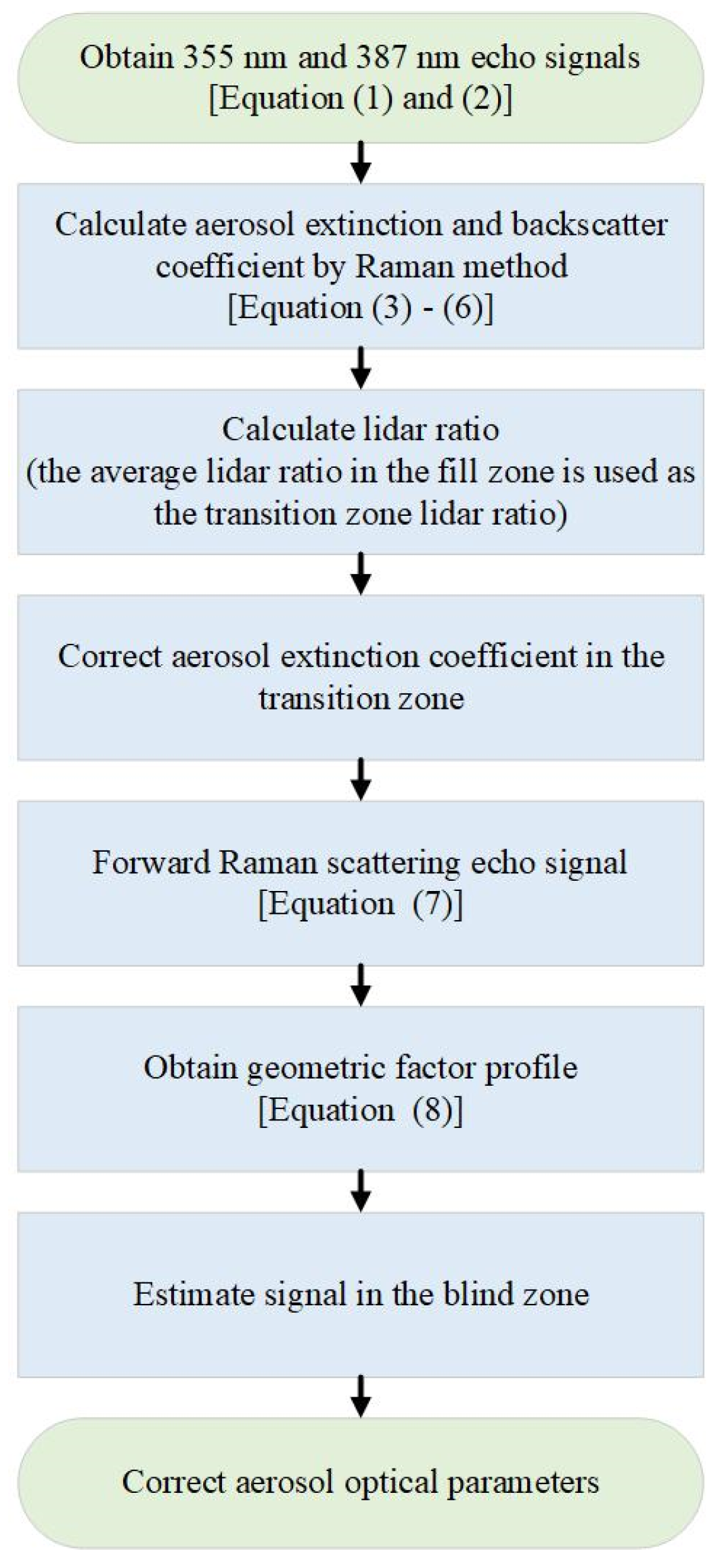
2. Geometric Factor Correction Algorithm

The emission wavelengths of the temperature and humidity profile lidar are 355 nm and 532 nm, with Mie scattering signals of 355 nm and 532 nm, vibrational Raman scattering signals of 387 nm and 407 nm, as well as pure rotational Raman scattering signals of 354 nm and 353 nm, which are received by a telescope and the subsequent optical path splitting. Due to the incomplete overlap between the emitted beam and the received field of view of the system, there is a geometric factor that results in the near-field signal being only partially received [15]. The geometric factor is 0 in the system’s blind zone since the telescope is not picking up the echo signal. The transition zone occurs when only a fraction of the echo signal reaches the receiving field of view and increases gradually with the detecting height; at this zone, the geometric factor smoothly moves from 0 to 1. The fill zone with a geometric factor of 1 is where the echo signal is fully received. The photodetector detects an inadequate and absent near-field signal, which encompasses the urban canopy layer intimately associated with human existence. In order to fulfill the high-precision detection aim of temperature and humidity profile lidar, the near-field signal must be corrected.

2.1. Mie Scattering Channel Correction Algorithm

The Mie scattering signal (355 nm) and vibration Raman scattering signal (387 nm) received by the temperature and humidity profile lidar are as follows [16]:

$$P(z,{\lambda }_E)=C_E{O}_E(z){\displaystyle \frac{{\beta }_a(z,{\lambda }_E)+{\beta }_m(z,{\lambda }_E)}{z^2}}\times \exp \{-2{\displaystyle {\int }_0^z[{\alpha }_a(z,{\lambda }_E)+{\alpha }_m(z,{\lambda }_E)]dz}\}$$

(1)

$$\begin{array}{l}P(z,{\lambda }_V)=C_V{O}_V(z){\displaystyle \frac{N_V(z)}{z^2}}{\displaystyle \frac{d\sigma (\pi )}{d\Omega }}\hfill \\ \hspace{1em}\hspace{1em}\hspace{1em}\hspace{1em}\hspace{1em}\times \exp \{-{\displaystyle {\int }_0^z[{\alpha }_a(z,{\lambda }_E)+{\alpha }_m(z,{\lambda }_E)+{\alpha }_a(z,{\lambda }_V)+{\alpha }_m(z,{\lambda }_V)]dz}\}\hfill \end{array}$$

(2)

where P(z, λ) represents the elastic scattering and vibrational Raman scattering echo signals at a distance of z, λ is the wavelength, C is the system constant, O(z) is the geometric factor, β(z) is the backscatter coefficient of aerosols (subscript a) and atmospheric molecules (subscript m) at the emission wavelength, N_V(z) is the number density of nitrogen molecules, dσ(π)/dΩ is the differential scattering cross-section of nitrogen molecules, and α(z) is the extinction coefficient of aerosols (subscript a) and atmospheric molecules (subscript m) at the emission wavelength and Raman wavelength. The subscripts E and V represent elastic scattering and vibrational Raman scattering, respectively.

From the above equation, it can be seen that the aerosol backscatter is independent of the nitrogen echo signal, which is mainly affected by the aerosol extinction coefficient. The aerosol extinction coefficient can be inverted using the Raman method, with no parameter assumptions to avoid introducing errors, as demonstrated by the relatively stable nitrogen molecule abundance in the atmosphere [17,18]:

$${\alpha }_a(z,{\lambda }_E)={\displaystyle \frac{1}{1+{(\frac{{\lambda }_V}{{\lambda }_E})}^{-A}}}\left\{{\displaystyle \frac{d}{dz}}[\ln {\displaystyle \frac{N(z)}{P(z,{\lambda }_V)z^2}}]-{\alpha }_m(z,{\lambda }_E)[1+{({\displaystyle \frac{{\lambda }_V}{{\lambda }_E}})}^{-4}]\right\}$$

(3)

where A is the Ångström exponent. The general value is between 0 and 4 [19], which can be calculated by the following equation [20]:

$$A(z)={\displaystyle \frac{\ln ({\beta }_a(z,{\lambda }_2)/{\beta }_a(z,{\lambda }_1))}{\ln ({\lambda }_1/{\lambda }_2)}}$$

(4)

To calculate the aerosol backscatter coefficient, the system can be calibrated using clear and cloudless nighttime high-altitude data with a very low aerosol content. The scattering ratio at 355 nm is approximately 1, and the scattering ratio at 532 nm is approximately 1.01 [17]. Therefore, the aerosol scattering ratio (defined as the ratio of total backscatter to molecular backscatter) can be calibrated as follows:

$$R(z,{\lambda }_E)={\displaystyle \frac{{\beta }_a(z,{\lambda }_E)+{\beta }_m(z,{\lambda }_E)}{{\beta }_m(z,{\lambda }_E)}}=C{\displaystyle \frac{P(z,{\lambda }_E)}{P(z,{\lambda }_V)}}{\displaystyle \frac{O_V(z)}{O_E(z)}}$$

(5)

The geometric factors of the two channels can be about equal during system design if the optical paths of the vibrational Raman scattering and Mie scattering channels are consistent. Consequently, the aerosol backscatter coefficient is:

$${\beta }_a(z,{\lambda }_E)={\beta }_m(z,{\lambda }_E)\times \left[C{\displaystyle \frac{P(z,{\lambda }_E)}{P(z,{\lambda }_V)}}-1\right]$$

(6)

As can be observed from the computation procedure above, the geometric factor does not affect the aerosol backscatter coefficient determined by the Raman method, and trustworthy signals can be obtained in the near-field region. Getting the lidar ratio is the next important step. The near-field extinction coefficient can be supplemented by multiplying the lidar ratio by the backscatter coefficient. To correct the extinction coefficient in the transition zone, the average lidar ratio at a given height in the fill zone is utilized. The forward vibration Raman scattering echo signal can be calculated by using the supplemented extinction coefficient:

$$P(z,{\lambda }_V)={\displaystyle \frac{N(z)}{z^2\cdot \exp \{{\alpha }_a(z,{\lambda }_E)[1+{(\frac{{\lambda }_V}{{\lambda }_E})}^{-A}]+{\alpha }_m(z,{\lambda }_E)[1+{(\frac{{\lambda }_V}{{\lambda }_E})}^{-4}]\}}}$$

(7)

The system geometric factor profile can be expressed as the ratio of the measured Raman scattering signal $P^{\prime }(z,{\lambda }_V)$ to the forward vibration Raman scattering echo signal:

$$O(z)={\displaystyle \frac{P^{\prime }(z,{\lambda }_V)}{P(z,{\lambda }_V)}}$$

(8)

The near-field fluorescence effect causes a “false signal” in the blind zone during lidar detection, which means that the geometric factor is never null. To differentiate the blind zone from the transition zone, a threshold that is near 0 must be specified. The profile of the standard aerosol extinction coefficient determined by the US standard atmosphere model crosses through the blind zone point when the aerosol extinction coefficient supplement is applied inside the blind zone. This can be accomplished by applying the theoretical slope approach for rectification. Figure 1 depicts the flow of the Mie scattering channel’s geometric factor correction procedure.

2.2. Raman Scattering Channel Correction Algorithm

There are two types of Raman scattering channels: vibration Raman scattering channels for humidity measurement and pure rotational channels for temperature measurement. Different calibration algorithms are needed because the optical structures in the receiving system vary. The wavelengths employed for humidity inversion in the vibrational Raman scattering channel are 387 nm and 407 nm, respectively, with a significant gap between the two wavelengths. As a result, a 45° color divider can be employed to split the echo beam during splitting system construction, transmitting 387 nm (P387) and reflecting 407 nm (P407), as seen in Figure 2. The geometric factors in the echo signals of the two shared receiving and emission routes are the same, as determined by employing photodetectors with the same performance, laser rangefinders, 6-D locators, and other tools to confirm that the receiving optical paths at 387 nm and 407 nm are consistent. As a result, the computed humidity quotient value (P407/P387) in the transition zone is trustworthy, and interpolation is only required to fill in the missing humidity data in the blind zone.

The high- and low-order wavelengths employed for temperature retrieval in the pure rotational Raman scattering channel are 353 nm (P353) and 354 nm (P354), respectively, which are in close proximity to the emission wavelength. A “Z”-shaped optical route was created for echo beam splitting in order to fully take advantage of the filter’s blue shift properties, as seen in Figure 3. The temperature quotient (P354/P353) will include the delay geometric factor since the path length of 353 nm is longer than that of 354 nm, resulting in a different geometric factor.

The pure rotational Raman scattering echo signal is as follows [21,22,23,24]:

$$\begin{array}{l}P(z,{\lambda }_R,T)=C_R{O}_R(z){\displaystyle \frac{N_R(z)}{z^2}}{\displaystyle \frac{112{\pi }^4}{15}}{\displaystyle \frac{g(J)hcB{[v_0+\Delta v(J)]}^4{\gamma }^2}{{(2I+1)}^{2}kT}}X(J)\exp [-{\displaystyle \frac{E(J)}{kT}}]\hfill \\ \hspace{1em}\hspace{1em}\hspace{1em}\hspace{1em}\hspace{1em}\times \exp \{-{\displaystyle {\int }_0^z[{\alpha }_a(z,{\lambda }_E)+{\alpha }_m(z,{\lambda }_E)+{\alpha }_a(z,{\lambda }_R)+{\alpha }_m(z,{\lambda }_R)]dz}\}\hfill \end{array}$$

(9)

where N_R(z) is the number density of nitrogen or oxygen molecules, g(J) is the weight factor related to nuclear spin I, h is the Planck constant, c is the speed of light, B is the rotational constant of the molecule at the ground state vibrational level, ν₀ is the frequency of the emitted laser, Δv(J) is the Raman scattering frequency shift, γ is the anisotropic parameter of molecular polarization intensity, k is the Boltzmann constant, T is the atmospheric temperature, and E(J) is the rotational energy of the same nuclear diatom with the ground state vibrational level rotational quantum number J. Based on this, the temperature quotient value is expressed as follows:

$$Q(z,T)={\displaystyle \frac{P_{low}(z,T)}{P_{high}(z,T)}}=C{O}_R(z){\displaystyle \frac{{\displaystyle \sum _{i=N_2,O_2}{\displaystyle \sum _{J_{low}}{N}_{R,i}(z)}{\tau }_{low}{\left(\frac{d\sigma (\pi )}{d\Omega }\right)}_i(J_i,T)}}{{\displaystyle \sum _{i=N_2,O_2}{\displaystyle \sum _{J_{high}}{N}_{R,i}(z)}{\tau }_{high}{\left(\frac{d\sigma (\pi )}{d\Omega }\right)}_i(J_i,T)}}}$$

(10)

where C is the system constant ratio, O_R(z) is the delay geometry factor, τ is the system optical efficiency, and dσ(π)/dΩ is the differential scattering cross-section of nitrogen or oxygen molecules. Due to the close wavelength of high-order and low-order Raman scattering signals, the atmospheric transmittance term is eliminated in the ratio. By using the spectral width of each channel filter and calibrating the received spectral line shape, the normalized transmittance can be obtained.

The theoretical high–low order differential scattering cross-section ratio can be determined using sounding temperature T; the following result can be obtained:

$$C{O}_R(z)={\displaystyle \frac{Q(z,T)}{\frac{{\displaystyle \sum _{i=N_2,O_2}{\displaystyle \sum _{J_{low}}{N}_{R,i}(z)}{\tau }_{low}{\left(\frac{d\sigma (\pi )}{d\Omega }\right)}_i(J_i,T)}}{{\displaystyle \sum _{i=N_2,O_2}{\displaystyle \sum _{J_{high}}{N}_{R,i}(z)}{\tau }_{high}{\left(\frac{d\sigma (\pi )}{d\Omega }\right)}_i(J_i,T)}}}}$$

(11)

The delay geometric factor O_R(z) can be obtained by calibrating the system constant C with measurement data from the fill zone in stable air conditions without temperature retrieval. The temperature quotient value is corrected using a delay geometric factor, and then an approximative quadratic polynomial fitting is carried out:

$$Q^{\prime }(z,T)=\exp ({\displaystyle \frac{a}{T^2}}+{\displaystyle \frac{b}{T}}+e)\iff T={\displaystyle \frac{-2a}{b\pm \sqrt{b^2-4a(e-\ln Q^{\prime }(z,T))}}}$$

(12)

where a, b, and e are calibration coefficients that can be used for the temperature calculation of continuous signal acquisition. Figure 4 depicts the flow of the Raman scattering channel’s geometric factor correction procedure.

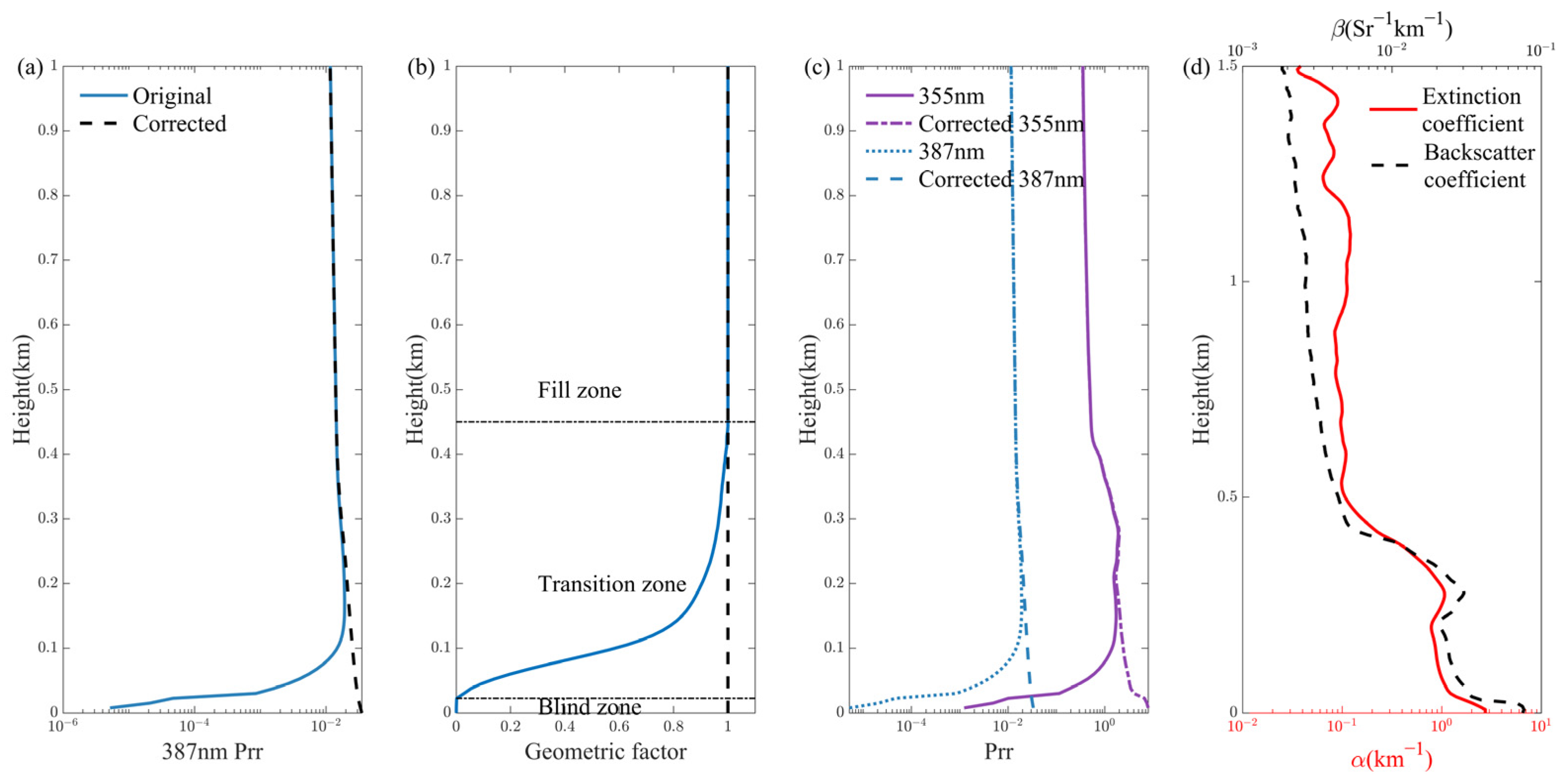
3. Experimental Analysis and Discussion of Geometric Factor Correction

The team’s self-developed temperature and humidity profile lidar was calibrated for the experiments, and the system parameters are shown in

Table 1. The key specifications of the lidar system.

Laser: Nd: YAG		Receiver: Newton Telescope
Wavelength/(nm)	355, 532	Diameter/(mm)	300
Energy/(mJ)	3.5, 1.5	Iris/(mrad)	1.0
Repetition rate/(Hz)	2000	Optical efficiency	0.3
Divergence/(mrad)	0.5	Interference filter bandwidth/(nm)	0.3–0.5
Temporal resolution/(min)	5	Range resolution/(m)	7.5
Data acquisition	AD + PC	Detector	PMT

. The aerosol extinction coefficient was measured by this lidar from 00:00 on 1 February 2024 to 03:30 on 2 February 2024, in Harbin (45°42′59.4″N, 126°37′54.5″E). The relative humidity and temperature were measured by this lidar from 00:00 on 26 December 2023, to 00:00 on 29 December 2023, in Guangzhou (23°6′5.5″N, 113°19′24.6″E). These were then compared and verified with atmospheric meteorological data from the Environmental Protection Agency and vertical data measured by a meteorological gradient tower (Canton Tower). The Environmental Protection Agency used the TH-NJD50 visibility meter to detect the atmospheric environment in real-time, with a detection range of 0–50 km (≤1 km ± 2%, ±10% > 1 km). The Canton Tower (23°6′31.4″N, 113°19′4.1″E) is located in Guangzhou City, and it has three air quality monitoring platforms at 118 m, 168 m, and 488 m [25,26,27]. The meteorological probes at the monitoring sites can measure atmospheric data such as temperature and relative humidity.

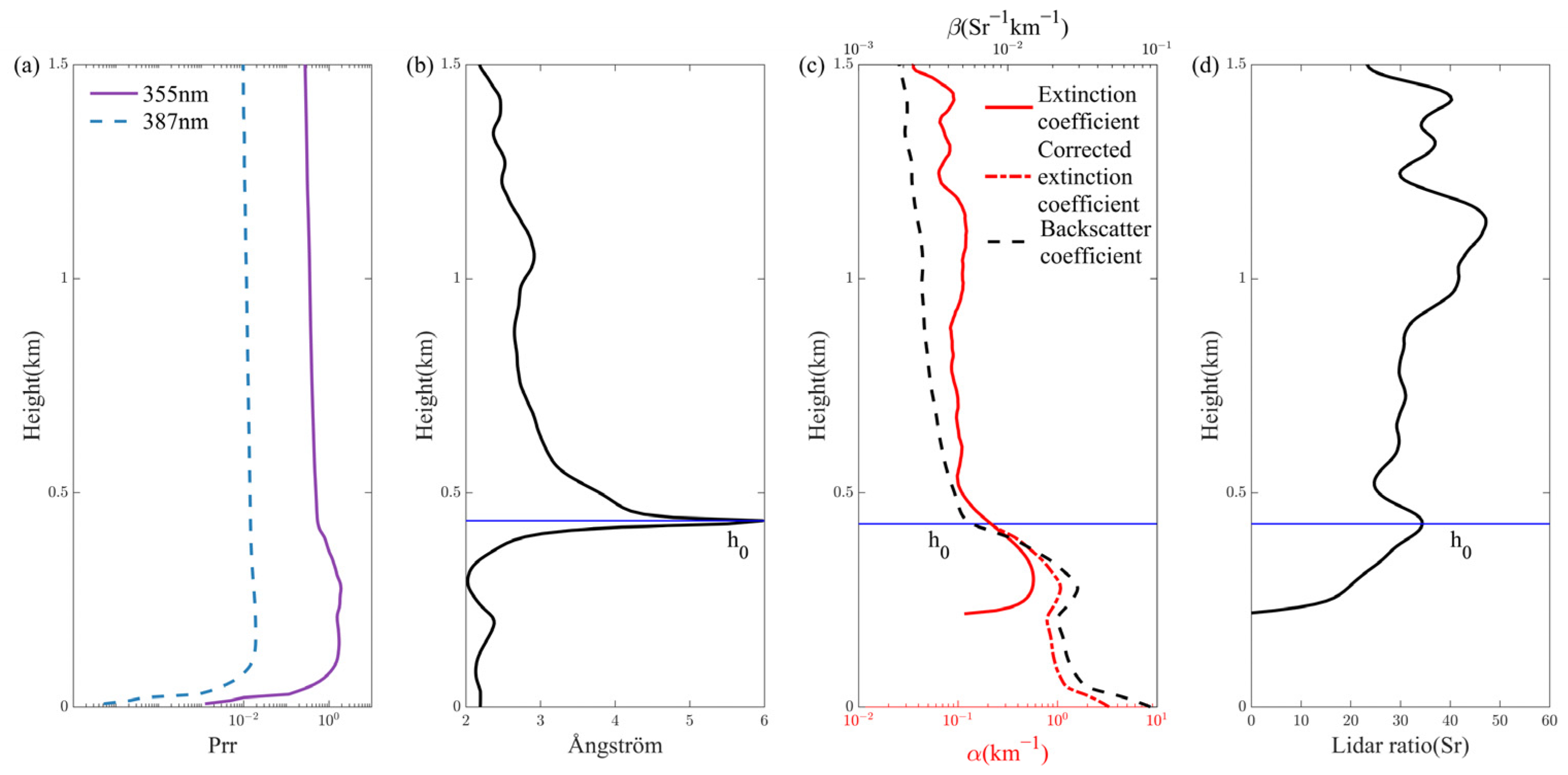
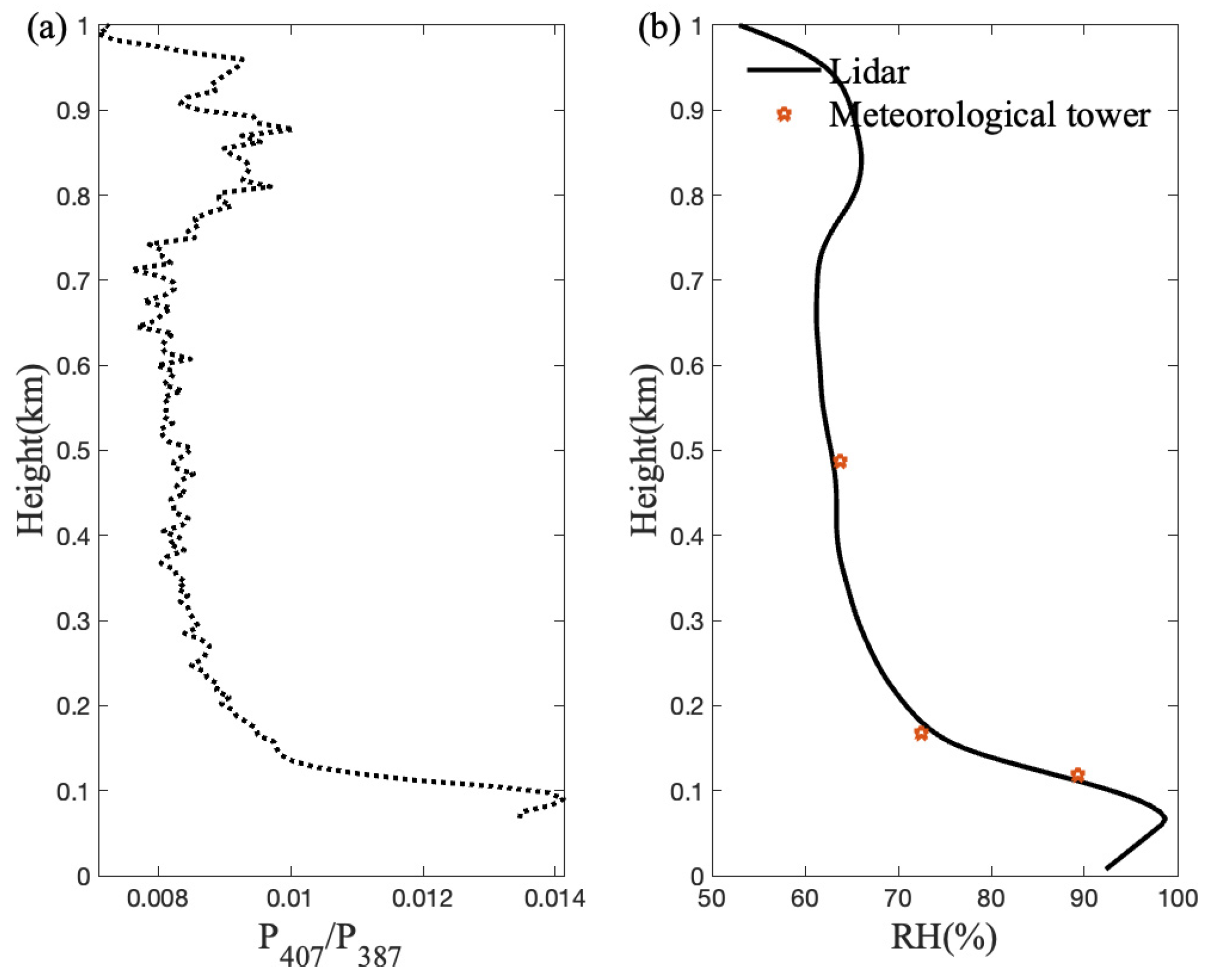
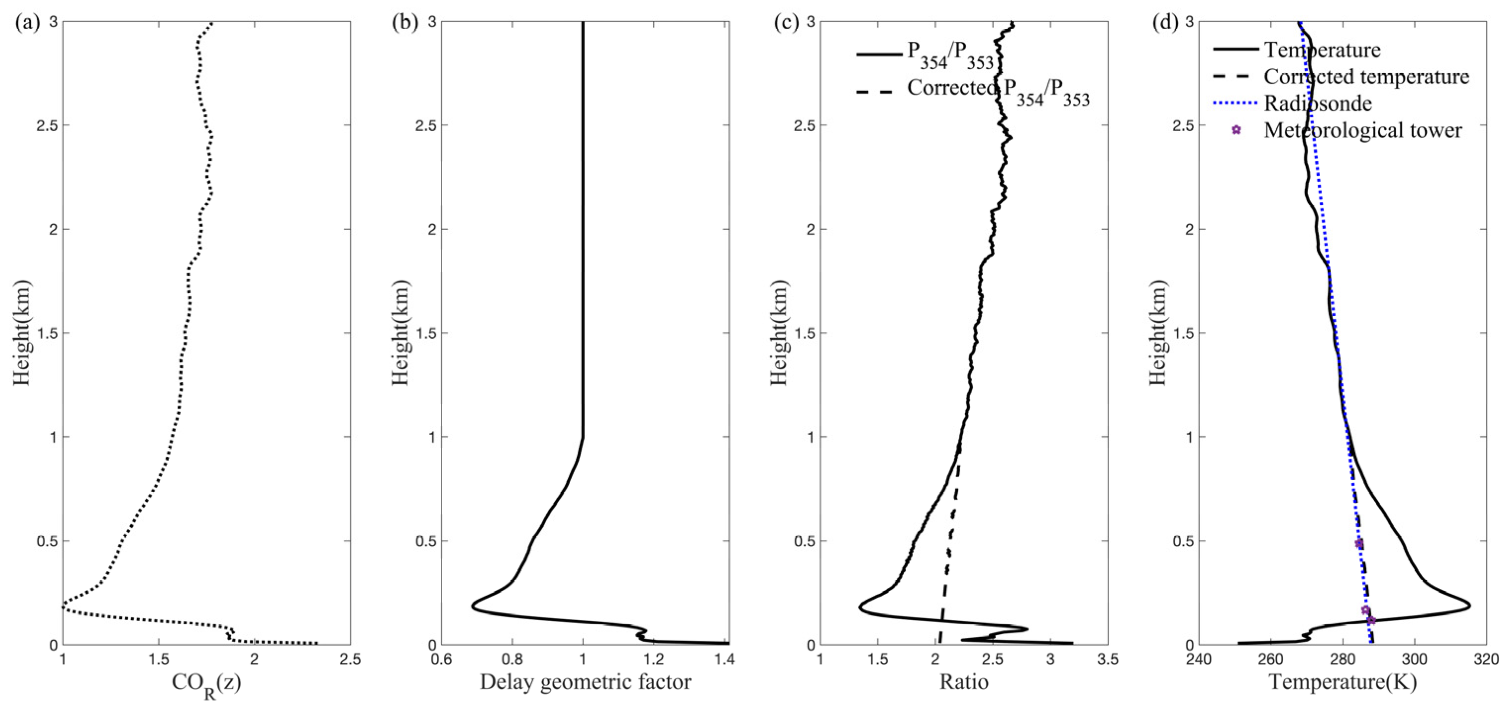
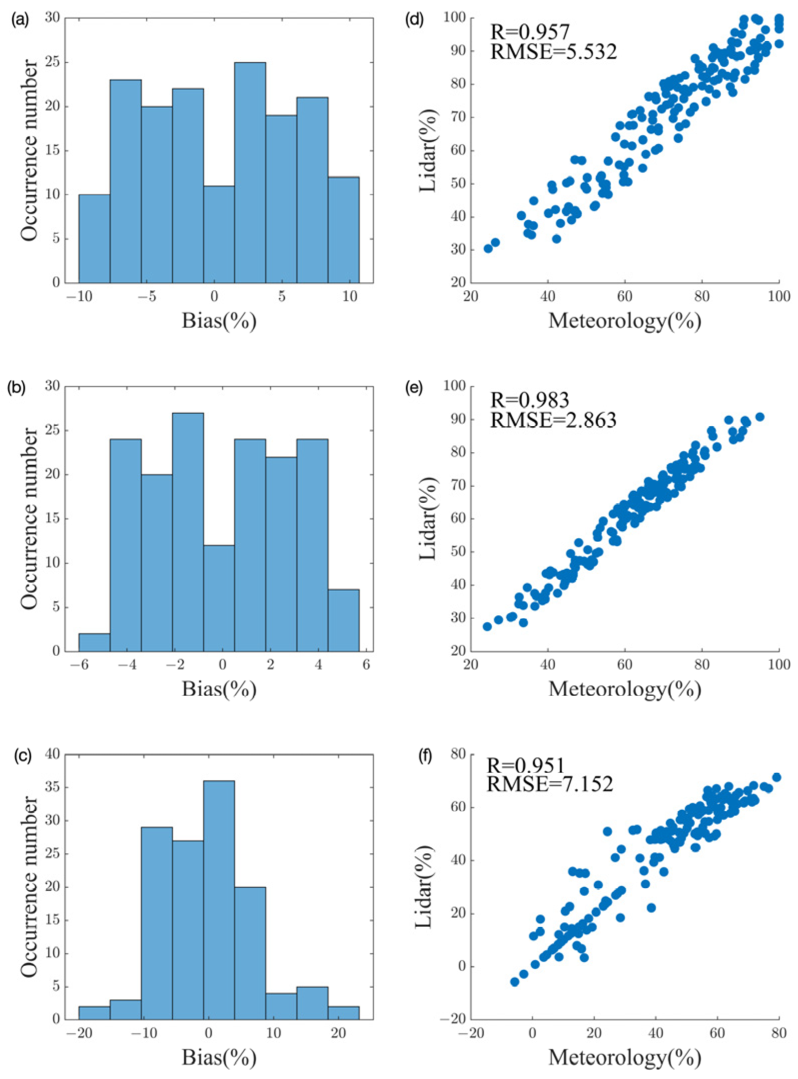
3.1. Analysis of Single-Profile Correction

Figure 5 displays the raw range-squared-corrected echo signal obtained using the temperature and humidity profile lidar. In the near-field region, the echo signal in Figure 5a exhibits an increasing trend with distance due to the geometric factor. The Ångström exponent, which is derived from the backscatter coefficients at 532 nm and 355 nm, is displayed in Figure 5b. The accuracy of the system when inverting aerosol optical characteristics can be enhanced by utilizing the fill zone’s average Ångström exponent. The profiles of the aerosol backscatter coefficient and extinction coefficient calculated via the Raman method are displayed in Figure 5c. Within 1.5 km, the Ångström exponent increased with the increased backscatter coefficient, which indicated that fine particles (with a size smaller than emission wavelength) may constitute the main component of aerosols. The backscatter coefficient is less impacted by the transition zone and is still valid in the near-field region, but the extinction coefficient steadily deteriorates below 0.435 km. Under the influence of the geometric factor, the extinction coefficient rapidly decayed, and negative values were calculated to cause the profile to break, resulting in null processing of invalid data. Due to the fact that, below 0.435 km, the variation of the aerosol extinction coefficient, Ångström exponent, and lidar ratio is much more affected by the geometric factor than by aerosol content, the first peak of optical parameters reflects the effect of the geometric factor on the transition zone and fill zone. Therefore, this height is selected as the initial value for the transition zone height h₀. Multiplying the backscatter coefficient by the average lidar ratio adds to the extinction coefficient profile in the transition zone. In Figure 5c, the dashed line displays the outcomes. The pattern of change for the augmented extinction coefficient is similar to the theoretical value change, and it is comparatively smooth and undistorted.

The vibration Raman scattering signal was forwarded using the preliminary corrected extinction coefficient, as indicated in Figure 6a. As a result, the corrected echo signal increased by four orders of magnitude, lowered the signal’s dynamic range, and progressively decreased with height. The geometric factor profile that the system measured can be determined by computing its ratio to the observed signal, as Figure 6b illustrates. The blind zone height is 0.0225 km, and the actual determined height of the transition zone is 0.45 km, which is near the initial height h₀ chosen in the preceding phase, suggesting that the inaccuracy of this correction approach is small. The optical parameter profile is supplemented and corrected using the theoretical slope method and the corrected echo signal, as shown in Figure 6c,d. The transition zone echo signal is corrected using the geometric factor profile. Using the collected extinction coefficient, Koschmieder’s law [28] allowed for the calculation of the atmospheric visibility, which came out as 2.52 km. The Environmental Protection Agency reported 3 km of atmospheric visibility. The two remained reasonably consistent with one another, confirming the geometric factor correction algorithm’s logic. As a result, the aerosol optical parameters, corrected for geometric factors, can accurately depict variations in the air environment inside the urban canopy layer, giving environmental protection agencies additional monitoring information and a more solid foundation for environmental governance. The average lidar ratio and the backscatter coefficient in the transition zone provide the forward-calculated vibration Raman scattering echo signal. The signal-to-noise ratio of the vibration Raman scattering signal determines the aerosol optical parameters’ accuracy, and the calibrated system constant may introduce errors as well. Weak signal noise can introduce some flaws in the inversion results when determining the aerosol extinction coefficient from the vibration Raman scattering echo signal. The theoretical slope method is used to augment the extinction coefficient within the blind zone, which is estimated using the US standard atmospheric model, which deviates somewhat from actual atmospheric changes. The signal correction in the transition zone and data supplementation within the blind zone are related to the height of the transition zone and the blind zone. The different heights of the two zones can affect the structure of the geometric factor, leading to deviations in signal correction. Therefore, determining the initial height of the transition zone is a crucial step. As mentioned earlier, the selection criterion for h₀ is the first peak height at which the Ångström exponent and lidar ratio undergo significant changes simultaneously.

The size, shape, and energy distribution of the light spot irradiated on the two photodetector surface sources are consistent, given that the optical path of the two humidity channels (P387 and P407) and the photodetectors’ performance are guaranteed to be consistent in the initial design of the subsequent optical path. By doing this, it is guaranteed that the two channels’ geometric factors are identical. The geometric factor in the humidity quotient no longer affects humidity retrieval because the geometric factors in the two-channel echo signals will be eliminated in the process of calculating the humidity quotient. Figure 7 displays the humidity data in the blind zone that was enhanced by the interpolation method. It is evident from Figure 7a that the humidity quotient value in the blind zone lacks a signal when the influence of near-field fluorescence is removed, preventing the further inversion of relative humidity. The humidity data enhanced by the interpolation method are displayed in Figure 7b. The relative humidity inversion results show good consistency when compared to the meteorological gradient tower’s data. The deviation between the two devices is very small. This confirms the validity of the interpolation method and can yield more precise humidity data for meteorological observations of the urban canopy layer.

For temperature channels, the geometric factors of high- and low-order pure rotational Raman scattering channels are not completely consistent due to the unequal optical paths of each channel; therefore, the delay geometric factor present in the temperature quotient cannot be directly eliminated. For the time difference caused by the optical path difference between the two channels when receiving echo signals, it is more appropriate to refer to this geometric factor as the delay geometric factor [29,30,31]. It is possible to completely remove the influence of Rayleigh–Mie scattering signals in the received pure rotational Raman scattering echo signals by choosing data with low aerosol content and cloudless weather for analysis. Figure 8 shows the transmittance curves of the measured high–low order channels and the narrowband filter used at the emission wavelength, with a high-order channel bandwidth of 0.5 nm at 353 nm and a low-order channel bandwidth of 0.3 nm at 354 nm. The transmittance of interference filters is above 60%. To fully suppress the crosstalk of Mie scattering signals, two interference filters were used in the optical path and rotated at a certain angle to position them. Based on the pure rotational Raman scattering spectra of oxygen molecules and nitrogen molecules at different temperatures, the quantum number of spectral lines used in the system can be determined. The differential scattering cross-sections of high-order and low-order channels can be further calculated using the temperature data obtained from sounding balloons.

Figure 9a,b display the computed CO_R(z) and delay geometry factor O_R(z). The detection data were processed using a filtering method because of the poor signal-to-noise ratio and weak pure rotational Raman scattering signal that was observed. Data beyond 2 km are used to calibrate the system constant profile. The O_R(z) profile shows that distortion from near-field fluorescence occurs in the blind zone and that, below 1 km, the value deviates from the theoretical value due to the influence of the delay geometric factor. The most obvious manifestation is that, as Figure 9c illustrates, the temperature quotient value approximates linearity with height in the fill zone, experiences severe deformation and attenuation in the transition zone, and false signals appear in the blind zone as a result of near-field fluorescence. The temperature retrieval results are displayed in Figure 9d both before and after correction. The delay geometric factor causes a large deviation of the uncorrected temperature from the sounding data, which makes it impossible to analyze the temperature variations within the urban canopy. The accuracy of near-field temperature retrieval is significantly increased by the corrected temperature profile, which agrees well with both the sounding and meteorological gradient tower data. This will help to advance the broad use of temperature and humidity profile lidar in atmospheric environment detection as well as the analysis of changes in the atmospheric environment within the urban canopy layer.

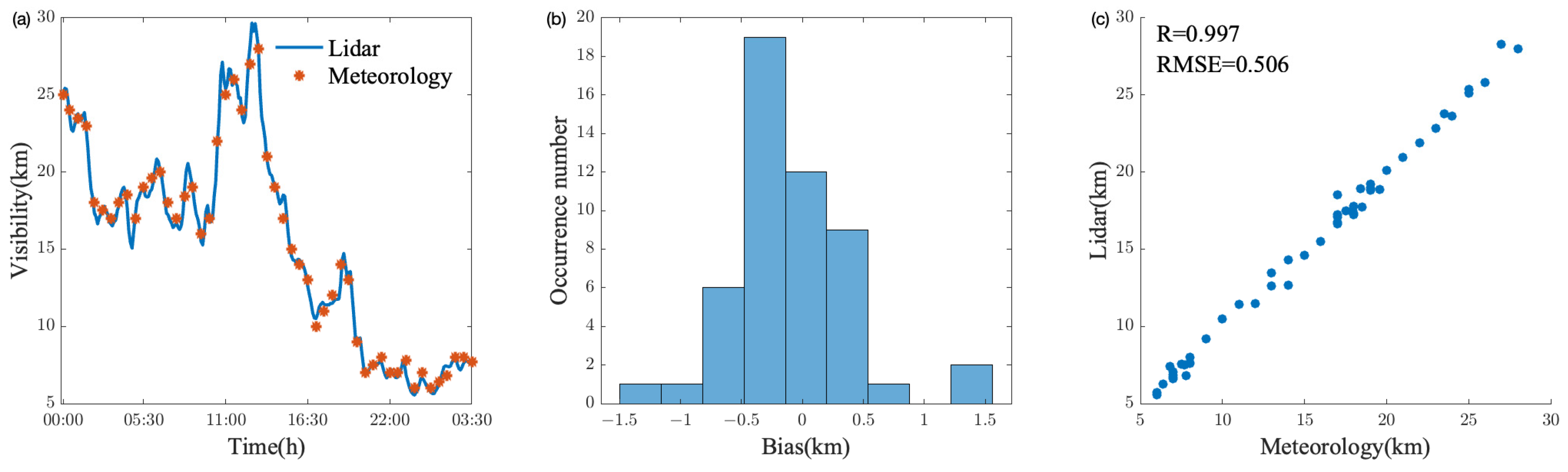
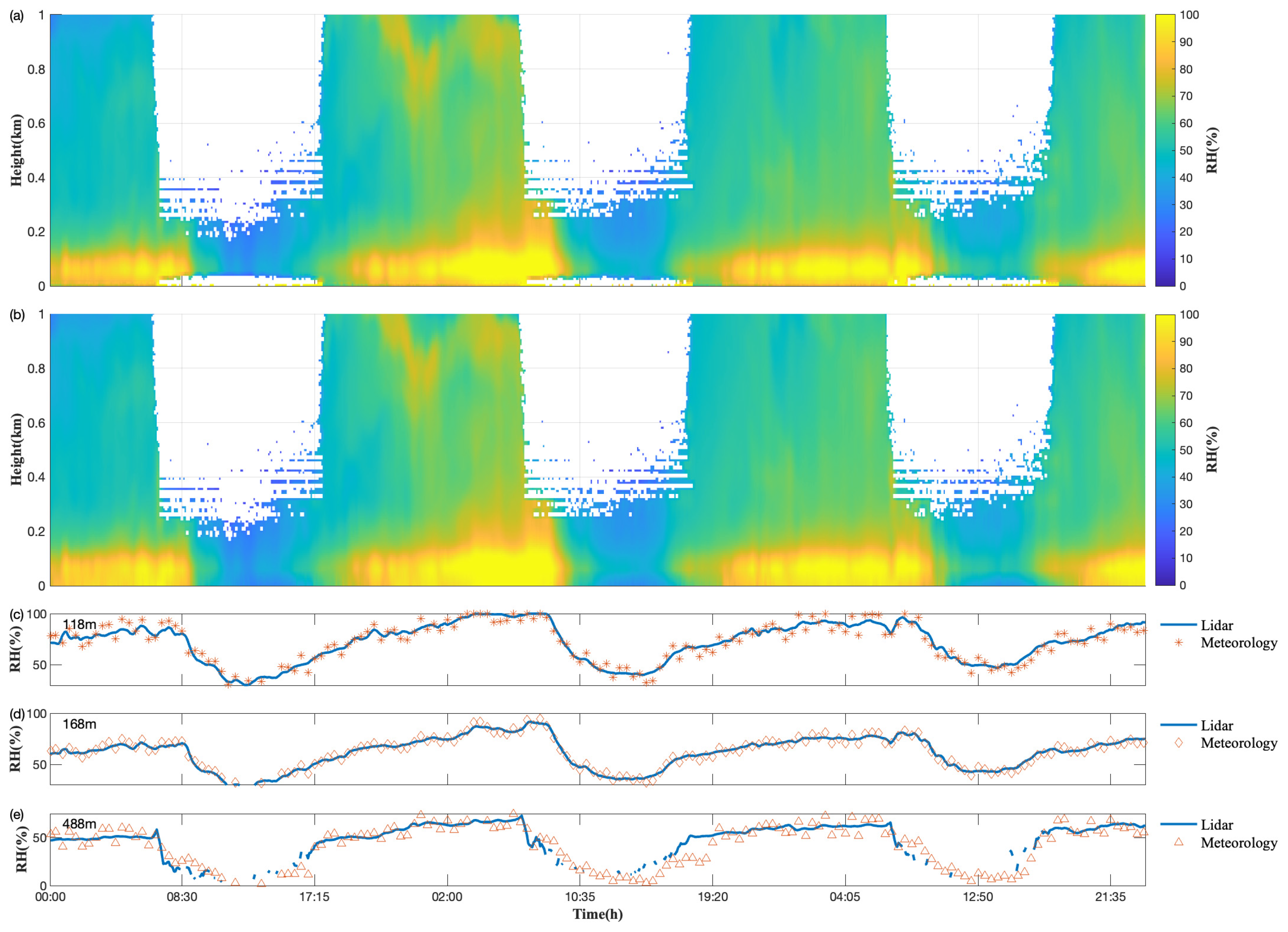
3.2. Analysis of Continuous Profile Correction

The aerosol extinction coefficient, humidity, and temperature profiles continuously collected by the temperature and humidity profile lidar were corrected and analyzed when the system parameters and emission path remained unchanged, in order to confirm the robustness and long-term stability of the proposed geometric factor correction algorithm. By comparing and statistically analyzing the observation data before and after calibration, lidar retrieval data, and fixed equipment measurement results, it has been proven that the calibration algorithm is effective in practical applications. The proposed algorithm can supplement the observation data within the urban canopy layer and improve the accuracy of lidar detection.

Figure 10 displays the spatiotemporal distribution of aerosol extinction coefficients as a pseudo-color map both before and after geometric factor correction. Figure 10a shows that the geometric factor alters aerosol optical characteristics below 0.5 km; invalid data occurred during the calculation, causing them to lose their spatiotemporal distribution. This makes it difficult to monitor the atmospheric environment of the urban canopy layer. The layered structure of aerosols is clearly depicted in Figure 10b, which rectified the transition zone signal using the geometric factor mentioned above. The spatial and temporal distribution of the corrected aerosol extinction coefficient clearly shows the process of particle transport and aggregation near the ground, allowing for the observation of the starting time of pollution aggravation. And the coherence between the supplemented data and the original data was smooth, without any jumps. This is of great value for analyzing the causes of pollution. Additionally, a model was added to the extinction coefficient within the blind zone. While it is an optimal approximation in the spatial domain, it can capture the aerosol transport mechanism in the temporal domain. Although the adaptability of the model is debatable, it is worthwhile using model data to obtain temporal aerosol variation patterns due to the very low height of the blind zone (below 30 m). More spatiotemporal evolution characteristics are shown by the corrected aerosol extinction coefficient close to the ground, offering trustworthy data for atmospheric particulate matter environmental monitoring in the urban canopy layer. The ground visibility was computed using the extinction coefficient’s inversion results, based on the atmospheric visibility data from the same period that were provided by the Environmental Protection Agency. Figure 11 displays the comparison findings, which further demonstrate the algorithm’s stability and robustness. The deviation between lidar retrieval results and device measurement data is mostly concentrated within 0.5 km, and the trend in visibility changes is the same, indicating that lidar measurement results have high accuracy. Compared to visibility meters that can only obtain visibility values at fixed heights within a fixed measurement interval, the lidar can obtain visibility values at any time and even at any height. The correlation between the two is as high as 0.997, with an RMSE of 0.506, which indicates a good consistency.

Figure 12 displays the relative humidity data that have been rectified by the interpolation method. It is evident by comparing the relative humidity before and after a correction that the interpolation method corrects the distorted data brought on by near-field fluorescence in addition to adding missing blind zone data. The distribution of water vapor does not jump within a short distance. As a result, the interpolation method can provide an approximation of the transmission mechanism and partially make up for the missing near-field data. Figure 12c–e displays the comparison results with the data recorded by the meteorological gradient tower sensors. The general consistency of the data’s changing variations attests to the long-term stability of the proposed algorithm. Figure 13 displays the correlation analysis and statistical deviation distribution histogram of humidity data collected by sensors at three different heights: 188 m, 168 m, and 488 m. At 488 m, there are partially missing and significant deviations in the lidar inversion data during the daytime period. This is due to the increasing sky background radiation and low single-pulse energy of the laser, which leads to a severe decrease in the signal-to-noise ratio of the echo signal. The signal-to-noise ratio of the vibrational Raman channel can be enhanced and the inversion accuracy can be improved by increasing the laser energy or suppressing the sky background radiation, such as by using interference filters or other filtering devices with stronger suppression capabilities. A correlation of more than 0.95 suggests that the calibration results of this method are trustworthy and useful for monitoring relative humidity in the urban canopy layer.

Figure 14 displays the temperature comparison before and after correction using the delay geometric factor to adjust the temperature quotient value and reinvert the temperature data. Figure 14a shows that the near-ground (below 0.2 km) data are warped and ineffectual, the inversion findings in the transition zone are biased and unreliable, and the temperature before rectification is impacted by the delay geometric factor, making it difficult to observe the day–night distribution in the time dimension. The corrected pseudo-color map of spatiotemporal temperature evolution is displayed in Figure 14b. It demonstrates notable daily temperature variations that follow the pattern of fluctuation in the atmospheric temperature field, and the temperature had not been amplified and was closer to the true values. There is also a clear presentation of the inversion layer close to 1 km. This provides the possibility to observe temperature field changes within the urban canopy layer. The proposed algorithm’s efficacy is confirmed by the good agreement between the corrected temperature and the meteorological gradient tower sensor’s measurement results, as seen in Figure 14c–e. The correlation analysis and statistical deviation distribution histogram between the lidar measurement data and the sensor measurement results at different heights are displayed in Figure 15. The accuracy of the detection is significantly increased when the temperature correlation at each height is better than 0.95. Studying and tracking the spatiotemporal evolution of the temperature of the urban canopy layer depends critically on the correction of the delay geometric factor.

4. Conclusions

To achieve the goal of monitoring atmospheric environmental changes within the urban canopy layer at all times, we have developed a temperature and humidity profile lidar to obtain aerosol optical parameters and temperature and humidity profile data within the urban canopy layer. Due to the hardware limitations of the system, the signal in the near-ground area was distorted by the geometric factor, which reduced the measurement accuracy and detection limit of the system.

In order to correct the echo signals, this paper proposed several solutions to the problem of the geometric factor influencing near-field signals in temperature and humidity profile lidar detection. The benefits of inverting aerosol optical properties using the Raman method were applied to the Mie scattering channel. The near-field extinction coefficient was supplemented by the measured backscatter coefficient, Ångström exponent, and lidar ratio. After solving the geometric factor through the forward calculation of the vibration Raman scattering signal, the Mie scattering channel echo signal was corrected. The model was applied to augment the optical parameters in the blind zone and the aerosol optical parameters were reinverted. Despite being a theoretical value that differs from the real atmosphere in space, it could represent the process of aerosol optical parameter transmission and evolution in the temporal dimension. The Environmental Protection Agency’s data on atmospheric visibility over the same period was compared with the ground visibility, which was determined through continuous signal collection. The results demonstrated the long-term stability and dependability of the proposed method.

For the vibration Raman scattering channel, the interpolation method was used to supplement the missing near-field relative humidity data. Although some accuracy was lost in the spatial dimension, the water vapor would not undergo severe distortion over a short distance, the evolution process of water vapor could still be reflected in the temporal dimension, and some inversion results have been corrected. Using the measured transmittance curve and normalized spectrum of the filter, combined with sounding data, the theoretical temperature quotient value was calculated. The ratio of the measured temperature quotient value to the delay geometric factor was used to reinvert the temperature through the corrected quotient value, solving the problem of sudden temperature changes and distortion in the near-field without affecting the signal observation results. The comparison between the temperature and humidity data measured by lidar and the measured data from meteorological gradient tower sensors showed that, while the lidar system remained unchanged, the proposed algorithm corrected the near-field temperature and humidity signal, improved the measurement accuracy of the system, and had high robustness and universality. The results indicate that the signals detected by lidar with Raman channels will no longer be affected by the geometric factor in the transition zone, and the signals in the blind zone will also have certain spatiotemporal significance, which is a significant innovation.

Several geometric factor correction algorithms carefully designed in this article aim to effectively correct the distorted echo signals in the transition region, thereby significantly improving the accuracy of aerosol optical parameters, relative humidity, and temperature data retrieval. The successful application of these innovative algorithms not only significantly reduced the detection limit of temperature and humidity profile lidar in effective data acquisition, but also significantly enhanced the overall detection efficiency and accuracy of the system. Compared to traditional observation methods such as radiosonde instruments and fixed monitoring probes, lidar stands out with its unparalleled high spatiotemporal resolution and continuous real-time monitoring capability. This technological advantage, combined with the algorithm proposed in this article, is particularly critical in dealing with complex and changing urban canopy layer meteorological environments. It makes lidar an ideal tool for capturing fine meteorological parameter changes and providing real-time and accurate data. Therefore, the research results of this article not only deepen the application potential of lidar technology in the field of meteorological detection, especially its practical value in urban canopy layer meteorological observation, but also lay a solid foundation for the widespread application and promotion of temperature and humidity profile lidar. This progress has profound significance and important application value for promoting the development of meteorological monitoring technology, improving the refinement level of urban environmental management, and enhancing the responsiveness to climate change.

References

1. Veselovskii, I.; Kolgotin, A.; Griaznov, V.; Müller, D.; Franke, K.; Whiteman, D.N. Inversion of multiwavelength Raman lidar data for retrieval of bimodal aerosol size distribution. Appl. Opt. 2004, 43, 1180–1195. [Google Scholar] [CrossRef] [PubMed]
2. Lange, D.; Behrendt, A.; Wulfmeyer, V. Compact Operational Tropospheric Water Vapor and Temperature Raman Lidar with Turbulence Resolution. Geophys. Res. Lett. 2019, 46, 14844–14853. [Google Scholar] [CrossRef]
3. Ji, H.; Zhang, Y.; Chen, S.; Chen, H.; Guo, P. Aerosol characteristics inversion based on the improved lidar ratio profile with the ground-based rotational Raman–Mie lidar. Opt. Commun. 2018, 416, 54–60. [Google Scholar] [CrossRef]
4. Hara, Y.; Nishizawa, T.; Sugimoto, N. Retrieval of Aerosol Components Using Multi-Wavelength Mie-Raman Lidar and Comparison with Ground Aerosol Sampling. Remote Sens. 2018, 10, 937. [Google Scholar] [CrossRef]
5. Teixeira, J.; Fallmann, J.; Carvalho, A.; Rocha, A. Surface to boundary layer coupling in the urban area of Lisbon comparing different urban canopy models in WRF. Urban Clim. 2019, 28, 100454–100470. [Google Scholar] [CrossRef]
6. Hu, S.; Wang, X.; Wu, Y.; Li, C.; Hu, H. Geometrical form factor determination with Raman backscattering signals. Opt. Lett. 2005, 30, 1879–1881. [Google Scholar] [CrossRef] [PubMed]
7. Hey, J. Determination of Lidar Overlap; Springer International Publishing: Berlin, Germany, 2015; pp. 81–106. [Google Scholar]
8. Gong, W.; Mao, F.; Li, J. OFLID: Simple method of overlap factor calculation with laser intensity distribution for biaxial lidar. Opt. Commun. 2011, 284, 2966–2971. [Google Scholar] [CrossRef]
9. Wang, W.; Gong, W.; Mao, F.; Pan, Z. Physical constraint method to determine optimal overlap factor of Raman lidar. J. Opt. 2018, 47, 83–90. [Google Scholar] [CrossRef]
10. Tomine, K.; Hirayama, C.; Michimoto, K.; Takeuchi, N. Experimental determination of the crossover function in the laser radar equation for days with a light mist. Appl. Opt. 1989, 28, 2194–2195. [Google Scholar] [CrossRef]
11. Kuze, H.; Kinjo, H.; Sakurada, Y.; Takeuchi, N. Field-of-view dependence of lidar signals by use of Newtonian and Cassegrainian telescopes. Appl. Opt. 1998, 37, 3128–3132. [Google Scholar] [CrossRef]
12. Su, J.; McCormick, M.; Liu, Z.; Leavor, K.H.; Lee, R.B.; Lewis, J.; Hill, M.T. Obtaining a ground-based lidar geometric form factor using coincident spaceborne lidar measurements. Appl. Opt. 2010, 49, 108–121. [Google Scholar] [CrossRef]
13. Wandinger, U.; Ansmann, A. Experimental determination of the lidar overlap profile with Raman lidar. Appl. Opt. 2002, 41, 511–514. [Google Scholar] [CrossRef] [PubMed]
14. Ji, H.; Chen, S.; Zhang, Y.; Chen, H.; Guo, P.; Chen, H. Calibration method for the reference parameter in Fernald and Klett inversion combining Raman and Elastic return. J. Quant. Spectrosc. Radiat. Transf. 2017, 188, 71–78. [Google Scholar] [CrossRef]
15. Ansmann, A.; Wandinger, U.; Riebesell, M.; Weitkamp, C.; Michaelis, W. Independent measurement of extinction and backscatter profiles in cirrus clouds by using a combined Raman elastic-backscatter lidar. Appl. Opt. 1992, 31, 7113–7131. [Google Scholar] [CrossRef]
16. Lv, M.; Zhao, C.; Wang, Q.; Li, Z. Feasibility study of water vapor and temperature retrieval using a combined vibrational rotational Raman and Mie scattering multi-wavelength lidar. In Proceedings of the Remote Sensing of the Atmosphere, Clouds, and Precipitation V, Beijing, China, 13–16 October 2014; Volume 9259. [Google Scholar]
17. Whiteman, D. Examination of the traditional Raman lidar technique. I. Evaluating the temperature-dependent lidar equations. Appl. Opt. 2003, 42, 2571–2592. [Google Scholar] [CrossRef]
18. Whiteman, D. Examination of the traditional Raman lidar technique. II. Evaluating the ratios for water vapor and aerosols. Appl. Opt. 2003, 42, 2593–2608. [Google Scholar] [CrossRef] [PubMed]
19. Ferrare, R.; Melfi, S.; Whiteman, D.; Evans, K.D.; Leifer, R. Raman lidar measurements of aerosol extinction and backscattering: 1. Methods and comparisons. J. Geophys. Res. Atmos. 1998, 103, 19663–19672. [Google Scholar] [CrossRef]
20. Song, I.; Kim, Y.; Baik, S.; Park, S.; Cha, H.; Choi, S.; Chung, C.; Kim, D. Measurement of Aerosol Parameters with Altitude by Using Two Wavelength Rotational Raman Signals. J. Opt. Soc. Korea 2010, 14, 221–227. [Google Scholar] [CrossRef]
21. Penney, C.; Peters, R.; Lapp, M. Absolute rotational Raman cross sections for N2, O2, and CO2. J. Opt. Soc. Am. 1974, 64, 712–716. [Google Scholar] [CrossRef]
22. Liu, F.; Yi, F. Lidar-measured atmospheric N2 vibrational-rotational Raman spectra and consequent temperature retrieval. Opt. Express 2014, 22, 27833–27844. [Google Scholar] [CrossRef]
23. Behrendt, A. Temperature Measurements with Lidar. In Lidar. Range-Resolved Optical Remote Sensing of the Atmosphere; Weitkamp, C., Ed.; Springer Series in Optical Sciences; Springer: New York, NY, USA, 2005; Volume 102, pp. 273–305. ISBN 0-387-40075-3. [Google Scholar]
24. Zenteno-Hernández, J.A.; Comerón, A.; Rodríguez-Gómez, A.; Muñoz-Porcar, C.; D’Amico, G.; Sicard, M. A Comparative Analysis of Aerosol Optical Coefficients and Their Associated Errors Retrieved from Pure-Rotational and Vibro-Rotational Raman Lidar Signals. Sensors 2021, 21, 1277. [Google Scholar] [CrossRef]
25. Fan, G.; Zhang, B.; Zhang, T.; Fu, Y.; Pei, C.; Lou, S.; Li, X.; Chen, Z.; Liu, W. Accuracy Evaluation of Differential Absorption Lidar for Ozone Detection and Intercomparisons with Other Instruments. Remote Sens. 2024, 16, 2369. [Google Scholar] [CrossRef]
26. Truong, T.; Cho, S.; Yun, C.; Sohn, H. Finite element model updating of Canton Tower using regularization technique. Smart Struct. Syst. 2012, 10, 459–470. [Google Scholar] [CrossRef]
27. Yi, T.; Li, H.; Wang, X. Multi-dimensional sensor placement optimization for Canton Tower focusing on application demands. Smart Struct. Syst. 2013, 12, 235–250. [Google Scholar] [CrossRef]
28. Koschmieder, H. Theorie der horizontalen Sichtweite. Beitrz Physd Freien Atm. 1924, 12, 33–53. [Google Scholar]
29. Chen, H.; Chen, S.; Zhang, Y.; Guo, P.; Chen, H.; Chen, B. Overlap determination for temperature measurements from a pure rotational Raman lidar. J. Geophys. Res. Atmos. 2016, 121, 2805–2813. [Google Scholar] [CrossRef]
30. Comerón, A.; Muñoz-Porcar, C.; Rodríguez-Gómez, A.; Sicard, M.; Dios, F.; Gil-Díaz, C.; Oliveira, D.C.F.d.S.; Rocadenbosch, F. An explicit formulation for the retrieval of the overlap function in an elastic and Raman aerosol lidar. Atmos. Meas. Tech. 2023, 16, 3015–3025. [Google Scholar] [CrossRef]
31. Ji, H.; Chen, S.; Zhang, Y.; Chen, H.; Guo, P. Determination of Geometric Factor for Ground-Based Raman-Mie Lidar with Bi-Static Configuration. Trans. Beijing Inst. Technol. 2019, 39, 644–649. [Google Scholar]
Figure 1. Flow chart for geometric factor correction of Mie scattering channel.
Remotesensing 16 02977 g001
Figure 2. Structural design of humidity chamber.
Remotesensing 16 02977 g002
Figure 3. Structural design of temperature chamber.
Remotesensing 16 02977 g003
Figure 4. Flow chart for geometric factor correction of Raman scattering channel.
Remotesensing 16 02977 g004
Figure 5. Single profile measurement results (00:12 on 2 February 2024, in Harbin): (a) Range-squared-corrected signal; (b) Ångström exponent; (c) aerosol optical parameters; (d) lidar ratio.
Remotesensing 16 02977 g005
Figure 6. Geometric factor calculation and signal correction. (a) Range-squared-corrected signal; (b) geometric factor (c) echo signal correction; (d) aerosol optical parameters correction.
Remotesensing 16 02977 g006
Figure 7. Humidity channel calibration (02:07 on 27 December 2023, in Guangzhou). (a) Measured quotient value; (b) Relative humidity correction.
Remotesensing 16 02977 g007
Figure 8. Normalized spectra and transmittance curves of pure rotational Raman scattering channels.
Remotesensing 16 02977 g008
Figure 9. Temperature channel calibration (21:16 on 28 December 2023, in Guangzhou). (a) COR(z); (b) delay geometric factor OR(z); (c) temperature quotient correction; (d) temperature correction.
Remotesensing 16 02977 g009
Figure 10. Pseudo-color map of the spatiotemporal distribution of the aerosol extinction coefficient (from 00:00 on 1 February 2024 to 03:30 on 2 February 2024, in Harbin). (a) Extinction coefficient before correction; (b) corrected and supplemented extinction coefficient.
Remotesensing 16 02977 g010
Figure 11. Comparison of visibility results. (a) Lidar data and meteorological data; (b) statistical error distribution between the lidar and meteorology (where the vertical axis represents the occurrence number); (c) correlation analysis.
Remotesensing 16 02977 g011
Figure 12. Relative humidity correction (from 00:00 on 26 December 2023 to 00:00 on 29 December 2023, in Guangzhou). (a,b) Relative humidity before and after calibration; (ce) comparison results of meteorology.
Remotesensing 16 02977 g012
Figure 13. Comparison of the relative humidity between Lidar data and meteorological data. (ac) Statistical error distribution at different heights (at 118 m, 168 m, 488 m); (df) correlation analysis.
Remotesensing 16 02977 g013
Figure 14. Temperature correction (from 00:00 on 26 December 2023, to 00:00 on 29 December 2023, in Guangzhou). (a,b) Temperature before and after calibration; (ce) Comparison results of meteorology.
Remotesensing 16 02977 g014
Figure 15. Comparison of the temperature between Lidar data and meteorological data. (ac) Statistical error distribution at different heights (at 118 m, 168 m, 488 m); (df) Correlation analysis.
Remotesensing 16 02977 g015