Insights into the Effects of Tile Size and Tile Overlap Levels on Semantic Segmentation Models Trained for Road Surface Area Extraction from Aerial Orthophotography

Abstract

Studies addressing the supervised extraction of geospatial elements from aerial imagery with semantic segmentation operations (including road surface areas) commonly feature tile sizes varying from 256 × 256 pixels to 1024 × 1024 pixels with no overlap. Relevant geo-computing works in the field often comment on prediction errors that could be attributed to the effect of tile size (number of pixels or the amount of information in the processed image) or to the overlap levels between adjacent image tiles (caused by the absence of continuity information near the borders). This study provides further insights into the impact of tile overlaps and tile sizes on the performance of deep learning (DL) models trained for road extraction. In this work, three semantic segmentation architectures were trained on data from the SROADEX dataset (orthoimages and their binary road masks) that contains approximately 700 million pixels of the positive “Road” class for the road surface area extraction task. First, a statistical analysis is conducted on the performance metrics achieved on unseen testing data featuring around 18 million pixels of the positive class. The goal of this analysis was to study the difference in mean performance and the main and interaction effects of the fixed factors on the dependent variables. The statistical tests proved that the impact on performance was significant for the main effects and for the two-way interaction between tile size and tile overlap and between tile size and DL architecture, at a level of significance of 0.05. We provide further insights and trends in the predictions of the extensive qualitative analysis carried out with the predictions of the best models at each tile size. The results indicate that training the DL models on larger tile sizes with a small percentage of overlap delivers better road representations and that testing different combinations of model and tile sizes can help achieve a better extraction performance.

1. Introduction

The successful application of deep learning (DL) to extract and map geospatial features from high-resolution aerial images demonstrates the potential of this artificial intelligence branch for geo-computing vision studies. Nonetheless, current limitations in available computational power force researchers in the field to divide the full aerial images into smaller image tiles with sizes from 256 × 256 pixels to 1024 × 1024 pixels—tile size refers to the pixel count or the number of pixels in an image (“image size” or “image resolution” are also commonly used terms in the specialized literature to refer to the $width\times height$ dimensions of a digital image) from the available data. Larger tile sizes include more scene information and can offer a richer learning context for a model. The cropped image tiles usually present no overlap; the tile/image overlap is measured in percentages and refers to the ratio of common pixels between adjacent tiles (it indicates the area percentage around an image border that is included in an adjacent image). The overlap can provide more aspects of the geospatial element to the model while only slightly increasing the correlation between the training samples.

The correct extraction of roads from aerial orthoimages is highly significant in the context of the rise of autonomous vehicles that require detailed road cartography. As of 2024, in Spain, the creation of road network cartography is still a manual process carried out within public agencies that involves human operators digitalizing road elements. In Sections 5 and 6 of [1] and Section 6 of [2], it was noted that higher rates of errors were present near tile borders even when DL road extraction solutions were trained on large-scale road surface area data of 256 × 256 pixels. This type of prediction artifact was also pointed out in Section 5 of [3]. For these reasons, it was decided to study the effects of tile size and tile overlap on performance, as additional information from larger tile sizes may help the DL implementation learning process by providing more semantic context, while small overlap percentages include additional information near the image borders that might help the learning process. Therefore, it could be beneficial for the model to be exposed to slightly shifted perspectives in the same region, potentially enhancing its generalization capacity.

This work is a continuation of [4], in which the impact of tile size and overlap was studied for the classification operation. Statistical analysis indicated that tile size significantly impacts the performance of road classification models, and models trained on tiles with a size of 1024 × 1024 provided the best performance. In this study, the effects of tile overlap and tile size levels on popular semantic segmentation models are quantified, evaluated, and qualitatively assessed. The goal is to provide additional insights into the significance of the performance metrics obtained and to analyze how the performance of a road surface area extraction changes based on the level of detail captured in the images. The starting premise of the study is “In extraction workflows of the road surface area with deep learning, semantic segmentation models that are trained on datasets with more semantic context (larger tile size) and additional information available near the image borders (higher tile overlap), achieve a higher performance of resulting models trained for semantic segmentation”.

In this work, the road surface area extraction from aerial imagery is tackled as a binary deep learning task and involves classifying pixels as “Road” or “No Road (Background)”, given a new orthoimage tile. For this task, information from the SROADEX dataset [5] was used for training the models, as it contains representative binary road information (approximately 700 million pixels labeled with the positive “Road” class) covering a representative area of approximately 8450 km² of the Spanish territory.

The objective is to study the effects of tile overlap and tile size on models trained for extraction of the surface area road elements and to identify optimal combinations that can improve the performance of future model implementations. This could be useful in the following period, given the expected rise of autonomous vehicles and their requirements for high-quality road maps. The work can also contribute to the exploration and optimization of training data generation to enable more efficient and improved models for geospatial element extraction. The main contributions of this study are summarized as follows:

• Three tile sizes and two overlap levels were explored and statistically studied in eighteen different training scenarios, given that the combinations of tile overlap, tile size, and semantic segmentation architecture were considered. Three different DL models for semantic segmentation were trained and tested on a very large scale to examine how these factors affect prediction performance.
• The metrics achieved by the trained models on unseen testing data (containing approximately 18 million pixels of the positive class) were statistically analyzed to study the differences between the mean performance and the impact of the training settings on the performance. The p-values were significant for the main effects and for the two-way interaction between tile size and tile overlap and between tile size and DL architecture, with performance significantly affected by the training scenario settings.
• A large-scale visual evaluation of the predictions on the test set was carried out to qualitatively analyze the results, provide further insights, and observe trends in the data. Afterward, an extensive discussion on the significance of the insights and future work directions is provided.

The remainder of this article is organized as follows. Section 2 presents the road surface area task from a mathematical perspective. Section 3 comments on works related to this study. Section 4 describes the training and testing data. Section 5 presents the training methodology applied. Section 6 and Section 7 present the quantitative, statistical analysis, and qualitative evaluation of the results delivered by the trained models, respectively. Section 8 presents a discussion of the implications of these results and comments on the uncertainty of the models. Lastly, Section 9 presents the conclusions of the study and future directions.

2. Problem Description

In binary supervised tasks, $n$ independent samples of $(X, Y)$ are processed with machine learning models. In geo-computer vision, binary classification tasks, $X_n$ represents the nth feature found in the available image space while $Y_n$ represents the nth label (with a value of 0, or 1). The goal of the training process is to obtain a classifier function $h$, that predicts $Y$ given $X$ with a low classification error (achieving zero error is not a practical expectation; the classification error cannot be eliminated (equal to zero), as the noise $\epsilon$ present in the data, $X$, implies that the data will not contain the information required to perfectly predict $Y$. The discriminative approach eliminates image classifiers that do not generalize well. The performance of any classifier $h$ is measured by its classification error, and the goal is to minimize it as much as possible with enough observations (as the size of the input data increases, the probability of driving the classification toward a minimum increase) and achieve a classifier that has a good prediction performance. As $Y\in \{0, 1\}$, it follows a Bernoulli distribution, and the regression function of $Y$ onto $X$ ($Y|X$) can be used to obtain a Bayes classifier function $h^{*}$ defined by a rule that assigns the label “0” when the computed value is lower than 0.5 and “1” when it is at least 0.5, but it is important to note that this is a simplification and the implementation of Bayes classifier may involve more complex decision rules [4,6,7].

As for the road surface area extraction operation, from a theoretical perspective, it is formulated as a semantic segmentation task where, given an input image, the goal is to predict a class label for each pixel (adapted from [7]). During training, the DL model will model a binary segmentation function to correctly tag each pixel of a random image variable $X=\{x_1,x_2, ..., x_n\}$ with one of the labels belonging to the label space $Y\in \{0, 1\}$ (i.e., “Road”/“Background”). Remotely sensed images and the complexity of the object studied imply that the input is not noise-free. Furthermore, the boundaries of the estimated object will not always coincide with the input image due to errors affecting the labeling process. Therefore, the inference error cannot be zero, and striving for an error-free model is not realistic.

The encoder-decoder learning structure enables the application of probability theory. A probability distribution, $p\left(y\right|X)$, can be specified ($X$ being the matrix of input features) to estimate the probability of a specific label assignment $y$, given an input image with $M$ pixels [8] (as defined in Equation (1)).

$$p\left(y|X\right)=\prod _{m=1}^{M}p\left(y_m\right|x_m)$$

(1)

In Equation (1), the probability $p\left(y\right|X)$ represents the uncertainty of the joint label assignment, where $p\left(y_m\right|x_m$) corresponds to the confidence of the model in assigning a label $y$ from $Y\in \{0, 1\}$ to a pixel $x_m$ (the probabilities are based on the current knowledge and training of the model). The encoder-decoder approach involves downsampling the size of the input tensor of dimensions, $height\times width\times depth (h\times w\times d)$, by means of convolutional layers to develop feature mapping of a smaller size and discriminate between the two classes, and upsample the representations afterward by means of transposed convolutions into a segmentation map with the same $h\times w$ output size.

Supervised learning tasks allow for the use of transfer learning [9] to leverage the weights from neural networks trained on datasets in the ImageNet Large Scale Visual Recognition Challenge (abbreviated ILSVRC, a classification task of 1000 categories with models trained on around 1.1 million images) [10], instead of applying a random initialization of the weights. This allows for potentially higher-quality results and faster convergence for a new given task [11].

3. Related Work

According to recent surveys [12], the extraction of the road transport network is one of the most addressed tasks in deep learning-based semantic segmentation of remote sensing images. This is considered complex due to the nature of the continuous geospatial object studied: different materials used in pavements, different widths and number of lanes, large curvature changes, no obvious borders, lack of markings, obstructions present in scenes, etc. In general, specialized works employ deep image segmentation techniques based on semantic segmentation models but focus on smaller, ideal-like, favorable scenarios, where the element tends to be grouped in clearly defined regions and features clearly defined borders.

Numerous studies have applied semantic segmentation for road surface area extraction. However, few studies have evaluated the effects of tile overlap and tile size. This section begins by reviewing the works that apply semantic segmentation for road surface area extraction and continues with a review of works that discuss the effect of tile size and tile overlap in semantic segmentation processes. The novel proposal from this study can be found at the intersection of these works.

In relation to the application of semantic segmentation techniques, works that apply convolutional neural networks (CNN), Transformers, and Generative Adversarial Networks can be found. Starting with CNN, DANet [13] provides a convolution kernel for convolutions on feature maps during upsampling to merge features of adjacent pixels and recover local information (target shapes, edges, or texture) while reducing errors near edges. Sharma et al. [14] propose a solution to reduce the network connectivity problem through gated convolutional techniques. This work also analyzes many publications from 2018 to 2023 from the point of view of the tile sizes used but does not reach any conclusion as to whether optimal configurations exist.

In relation to the use of Transformers, Xiong et al. [15] propose a segmentation algorithm that incorporates angle prediction and angle feature fusion modules and adds angle constraints specific to roads. The experimental data is obtained from the Deep Globe public dataset, which is divided into tiles of 512 × 512 pixels with a sliding window of 256 × 256 pixels. Seg-Road [16], using Deep Globe, proposes a transformer structure to improve road segmentation that also features a convolutional neural network (CNN) structure. Furthermore, a structure to improve the connectivity of road segmentation and the quality of predictions is proposed; however, the authors claim that the segmentation of adjacent roads needs improvement. Instead of providing feature fusion at the encoder-decoder level, the approach from this study designs overlap between adjacent image tiles to provide continuity in image borders.

In the field of GAN network applications, GA-Net [17] has been proposed to enhance road connectivity. GA-Net introduces a feature aggregation module to enhance spatial information at multiple scales. The authors trained their model on the DeepGlobe, Massachusetts, and SpaceNet Road Dataset and achieved competitive F1-scores. Moreover, the solution proposed by Abdollahi et al. [18], also based on GAN networks (and using the Massachusetts road image dataset), allows better preservation of road borders and handling of occlusions and shadows. In [19,20], conditional GAN models were proposed for post-processing and improving the road representations extracted with semantic segmentation using image-to-image translation and deep inpainting techniques, respectively.

None of the previous papers carried out a study for different sizes of tiles or used various overlap techniques in their solutions to solve the problem of road network connectivity at edges. Regarding works evaluating the effects of tile size, there are some works outside the scope of remote sensing (such as [21]) that approach the effect of tile sizes for model prediction, concluding that “larger tile sizes yield more consistent results and mitigate undesirable and unpredictable behavior during model inference”. In the field of remote sensing, there are solutions that address the problem of tile size in their experiments. For example, Zhang et al. [22] generate smaller images of the ISPRS Vaihingen dataset (from 480 × 480 pixels input to 224 × 224 pixels output) and experiment with other input data such as 572 × 572 pixels and justify the use of tiling and padding to avoid overflowing video memory during training, while also recommending on the use of data from the image edge.

Other works ([23,24]) use machine learning-based attention methods to prioritize features of higher significance and fade those of lower priority. Tao et al. [25] model the input image at three scales; the attention learned at larger scales relates to smaller details, while the attention at smaller scales modeled more significant structures to enable a better segmentation of the object sizes considered.

In relation to the works that study how tile connectivity improves according to different overlap techniques, the work of Huang et al. [26] can be mentioned, where the challenges of tiling and stitching segmentation outputs for remote sensing are analyzed. The results indicate that using a zero-padding strategy in the tiling approach causes undesired prediction variability in image edges. These findings have led to subsequent works on image segmentation in tiles [21], considering the limitations of zero padding, and overlap in the input tiles.

Neupane et al. [27] published a review of papers on semantic segmentation of urban features in satellite images with DL and established that 18 of the 71 papers reviewed use overlap techniques (mostly 50% overlap), but only the work of Yue et al. [28] perform a calculation to optimize the percentage of overlap, in this case through Gaussian functions. Other works [29] use a sliding window with different overlapping ranges and compare the precision of the results. One of the latest works by Hu et al. [30] applied seven levels of overlap (from 0 to 65%), concluding that larger overlaps increased performance (up to the saturation value of 55%) but also incurred a higher computational cost.

4. Data

The training data used are based on the SROADEX dataset [5], which contains RGB (Red, Green, Blue) aerial orthophotographs from Spain (representative data from different regions featuring diverse types of scenery). The data is produced by Spanish public agencies and features a spatial resolution of 0.5 m. Using a large dataset that features representative information from various conditions is particularly important for training and evaluating deep learning models for road segmentation to ensure high performance and the statistical significance of the results.

The orthoimages are distributed by the National Geographical Institute of Spain, and its producers state that standardized, rigorous procedures were applied to capture and process the data (orthorectification, radiometric, and topographical corrections) before distributing the product. The orthoimage data from SROADEX are labeled with binary road information at the pixel level (ground truth masks), which enables the supervised extraction of the road with semantic segmentation models. More details regarding the data can be found in the “Data” section of [4] and in Section 2 of [5].

The SROADEX data were re-split to follow the tile sizes and overlaps considered in this study, resulting in six different data combinations: (1) 256 × 256 pixel tiles with no overlap, (2) 256 × 256 pixel tiles with 12.5% overlap, (3) 512 × 512 pixel tiles with no overlap, (4) 512 × 512 pixel tiles with 12.5% overlap, (5) 1024 × 1024 pixel tiles with no overlap, and (6) 1024 × 1024 pixel tiles with 12.5% overlap. To avoid processing tiles featuring extremely unbalanced classes, a rule was applied to eliminate tiles where road segments within had a length smaller than 25 m. Afterward, the resulting data were divided with a criterion of 95:5% to obtain the training and validation sets (featuring approximately 700 million pixels of the positive “Road” class at each tile resolution).

The test set is represented by data from a novel region from Palencia, Spain, that was labeled to objectively assess the generalization capacity of the DL models and contains around 18 million pixels of the positive “Road” class. The labeled test area was split afterward to generate tiles at the three tile sizes considered (with no overlap) and compute the models’ performance metrics. The distribution of the data used in this study can be found in

Table 1. Distribution of the image tiles (and the number of pixels corresponding to each class) in the training, validation, and test sets for the binary semantic segmentation of roads using DL models.

Tile Size (Pixels)	Tile Overlap (%)	Set	No. Images	No. Pixels (per Class)
				Road	No Road (Background)
256 × 256	0%	Train	237,919	672,864,947	14,919,394,637
		Validation	12,523	35,644,583	785,062,745
		Percentage of data		4.32%	95.68%
	12.5%	Train	312,092	902,912,960	19,550,348,352
		Validation	16,426	47,987,916	1,028,506,420
		Percentage of data		4.42%	95.58%
	Test set (novel area, no overlap)		7708	18,158,800	486,992,688
	Percentage of data			3.59%	96.41%
512 × 512	0%	Train	90,475	669,081,651	23,048,396,749
		Validation	4762	34,773,408	1,213,556,320
		Percentage of data		2.82%	97.18%
	12.5%	Train	118,078	901,745,879	30,051,693,353
		Validation	6215	48,197,575	1,581,027,385
		Percentage of data		2.92%	97.08%
	Test set (novel area, no overlap)		3110	18,137,722	797,130,118
	Percentage of data			2.22%	97.78%
1024 × 1024	0%	Train	27,705	661,863,036	27,188,935,044
		Validation	1457	35,975,504	1,491,799,728
		Percentage of data		2.38%	97.62%
	12.5%	Train	36,034	891,014,527	36,893,373,057
		Validation	1897	47,973,497	1,941,175,175
		Percentage of data		2.36%	97.64%
	Test set (novel area, no overlap)		955	18,150,383	983,239,697
	Percentage of data			1.81%	98.34%

Notes: (1) Six different training and validation sets were generated for each combination of tile size and overlap using binary road information from the SROADEX dataset that was applied with a criterion of 95:5% (approximately 700 million pixels of the positive class “Road” at each tile size level). (2) The test set contains information from a novel, representative area from Palencia (Spain) that was not modeled during training. (3) Considering the spatial resolution of 0.5 m of the aerial imagery, the area covered by an image tile increases from approximately 0.016 km² to 0.065 km² and to 0.262 km² for tile sizes of 256 × 256, 512 × 512, and 1024 × 1024 pixels, respectively.

, while Figure 1 illustrates samples of aerial orthoimages and ground truth masks from the available data (in three tile sizes that were considered in this study).

In Table 1, it can be observed that the road extraction task involves processing highly unbalanced classes (very high percentages of the “Background” class) due to the natural underrepresentation of the road in a scene, particularly at higher sizes, when the image tiles contain more information (larger areas) but feature less road coverage. For example, the percentage of pixels labeled as “Road” in the training set decreases from approximately 4.32% in the data scenario of tiles with 256 × 256 pixels with no overlap to approximately 2.38% for the data scenario of tiles of 1024 × 1024 pixels with no overlap, while the “Background” class increases from 95.68% to 97.62% for the same data scenarios mentioned previously. Similar values can also be observed in the test set, and it is expected that this experimental design enables the investigation of the correlation between the amount of scene information and model performance.

5. Training Method

The study involves classifying pixels as “Road” or “No Road (Background)” and was tackled with deep learning methods for semantic segmentation. The semantic segmentation models considered follow the encoder-decoder learning structure (where the input is downsized to extract the representations that impact the performance, up to a bottleneck, where the processed is reversed and the feature maps are resized to the size of the input), [31,32]. The architecture–backbone configurations considered are U-Net [33]—Inception-ResNet-v2 [34], U-Net—SEResNeXt50 [35], and LinkNet [36] coupled with EfficientNet (b5 variant) [37]. These semantic segmentation models represent the state-of-the-art in the field and have proven their performance in relevant works specialized in geo-computer vision for large-scale extraction of geospatial elements [2,3].

By training these three DL models on the six data scenarios described in Section 4, a total of eighteen training scenarios were obtained (presented in

Table 2. Training scenarios considered for binary semantic segmentation of road surface areas using deep learning models.

Training Scenario ID	Semantic Segmentation Model	Tile Size (Pixels)	Tile Overlap (%)
1	U-Net—Inception-ResNet-v2	256 × 256	0
2			12.5
3	U-Net—Inception-ResNet-v2	512 × 512	0
4			12.5
5	U-Net—Inception-ResNet-v2	1024 × 1024	0
6			12.5
7	U-Net—SEResNeXt-50	256 × 256	0
8			12.5
9	U-Net—SEResNeXt-50	512 × 512	0
10			12.5
11	U-Net—SEResNeXt-50	1024 × 1024	0
12			12.5
13	LinkNet—EfficientNet-b5	256 × 256	0
14			12.5
15	LinkNet—EfficientNet-b5	512 × 512	0
16			12.5
17	LinkNet—EfficientNet-b5	1024 × 1024	0
18			12.5

), each combination of model, size, and overlap being considered a unique training scenario. This comprehensive approach enables a deeper insight into the interaction of these factors and their effects on performance and identifies the best combinations.

The training scripts for the DL models considered in this study were implemented using the “Segmentation Model” library version 1.0.1 [38] (based on Keras version 2.2.4 [39] and TensorFlow version 1.14.0 [40]). The experiments were conducted on an Ubuntu 22.04 server equipped with an NVIDIA V100-SXM2 GPU (NVIDIA, Nvidia Corporation, Santa Clara, CA, USA) with 16 GB of VRAM and all the software requirements installed. The training and evaluation codes, together with the test data and the best road extraction models, are available in the Zenodo repository [41] under the CC-BY 4.0 license.

The training task is to correctly predict a single feature per pixel (“Road“ or “Background”) in the output mask. The image data available were normalized from [0, 255] to [0, 1] to reduce the scale of the input features and avoid computation with large numbers. A series of transformations were applied to the input training images (such as random flips and rotations, color, and contrast adjustments) as data augmentation strategies with the same small parameter values in all experiments to increase the diversity of the training data. The batch size was the maximum allowed by the GPU’s capacity.

Transfer learning was applied to weight initialization so that the models could start the weight learning from ImageNet during ILSVRC [10] (commented in Section 2) and ensure the reuse of the features learned on this large dataset as a starting point. However, fine-tuning was applied so that the weights of the model were updated during training to learn the useful features for the road surface area extraction task.

A combination of binary cross-entropy and Jaccard loss functions was applied as loss (as defined in Equation (2)) to encourage the model to correctly predict the labels at the pixel level and to produce class predictions that have a high overlap with the ground truth masks (to capture the structure of the segmentation masks). In Equation (2), the combined loss of a model, $\mathcal{L}(y,\widehat{y})$, is calculated as a weighted sum of the two individual losses (defined in Equations (3) and (4)) to the final cost value, α represents the weight factor that balances the contribution of each component (its default hyperparameter value is tuned empirically by the library developers), while “$\cdot$” indicates the element-wise multiplication. The binary cross-entropy (BCE) function component is defined in Equation (3) and is commonly used in binary classification problems, while the Jaccard loss component is defined in Equation (4) and is extensively used for training DL models for image segmentation tasks as it is a good indicator of the overall quality of the segmentation.

$$\mathcal{L}(y,\widehat{y})=\alpha \cdot {\mathcal{L}}_{BCE}(y,\widehat{y})+(1-\alpha )\cdot {\mathcal{L}}_{Jaccard}(y,\widehat{y})$$

(2)

$${\mathcal{L}}_{BCE}(y,\widehat{y})=-{\displaystyle \frac{1}{N}}\sum _{i=1}^N[y_i\cdot log({\widehat{y}}_i)+(1-y_i)\cdot log(1-{\widehat{y}}_i\left)\right]$$

(3)

$${\mathcal{L}}_{Jaccard}(y,\widehat{y})=1-{\displaystyle \frac{\sum _{i=1}^N{y}_i\cdot {\widehat{y}}_i}{\sum _{i=1}^N{y}_i+\sum _{i=1}^N{\widehat{y}}_i-\sum _{i=1}^N{y}_i\cdot {\widehat{y}}_i}}$$

(4)

In Equation (3), $y$ is the true label (0 or 1, “Road” or “Background”), $\widehat{y}$ is the predicted label (probability between 0 and 1, where a threshold of 0.5 is used to determine the class value) while $N$ is the number of samples, $log$ denotes the natural logarithm. Therefore, the binary cross-entropy loss (${\mathcal{L}}_{\mathrm{B}\mathrm{C}\mathrm{E}}$) measures the error of a prediction when the output is expected to be a probability value between 0 and 1 and penalizes the model when it makes a wrong prediction with high confidence, treating each pixel as an independent binary classification problem and calculating the error accordingly.

In Equation (4), $y$ is the pixel class value in the ground truth mask, $\widehat{y}$ represents the corresponding pixel class value in the predicted mask, while $N$ represents the number of pixels in the mask. Therefore, the Jaccard loss (${\mathcal{L}}_{Jaccard}$) measures the similarity between predicted and ground truth masks, a lower loss indicating a higher overlap between the predicted and corresponding ground truth masks.

The computed cost value (calculated at the end of each epoch) was optimized using Adam with a starting learning rate of 0.001. Because of the pronounced class imbalance between the “Road” and “No Road (background)” classes, additional balancing techniques were applied for correct training and to avoid models biased toward the positive class. In this regard, the IoU score was monitored, and early stopping and reduction of learning rate strategies were applied to reduce the learning rate by a factor of 10 up to a minimum of 0.00001 or stop the training when the monitored metric had not improved for ten epochs, to prevent overfitting and help model convergence.

Finally, similar to the training methodology from [4], to isolate and reduce the effect of the randomness associated with deep learning model convergence and to compute statistical measures, in the experimental design, it was established to carry out a minimum of three experiment iterations for each training scenario from Table 2. This training design, with N = 3 samples at the training scenario level (statistically analyzed in Section 6.1), achieves a stronger reflection of the population size. Specifically, it enabled the analysis of performance metrics with $N=18$ samples when grouped by tile size, $N=27$ samples when grouped by tile overlap, and $N=18$ when grouped by semantic segmentation architecture (as detailed in Section 6.2).

6. Results

The loss defined in Section 4 (Equations (2)–(4)) measures how well the predictions of the models align with the true values, with a lower loss value indicating better performance. However, in the context of severe class imbalance (with road pixels occupying only about 3% of the total), additional performance indicators must be computed. The IoU score (defined in Equation (5) in terms of True Positive (TP, road pixels correctly identified as “Road”), False Positive (FP, background pixels incorrectly identified as belonging to the “Road” class), and False Negative (FN, road surface area pixels incorrectly identified as “Background”) values of the confusion matrix) measures the overlap between the predicted and true positive classes (is calculated as the division between the area of intersection and the area of the union of the predicted and the actual “Road” labels); a high IoU score (superior to 0.5) indicates the model that correctly identifies the positive class (“Road”, underrepresented in this case).

Precision (defined in Equation (6)) measures the proportion of correct “Road” predictions among all the positive predictions. A higher precision indicates fewer false positives, but it is important to consider that a model can achieve high precision by being overly conservative in its positive predictions. Recall (also called the sensitivity or true positive rate, defined in Equation (7)) measures the proportion of actual positives that were correctly identified. A higher recall indicates fewer false negatives, but note that a model with high recall could also achieve it by overpredicting the positive class. For these reasons, the F1 score (defined in Equation (8)), which indicates the harmonic mean of precision and recall, is also computed (it is a recommended performance indicator in tasks where severe class imbalance is present). Note that none of the metrics defined in Equations (5)–(8) account for the True Negatives (TN, which indicates the correct prediction of the majority “Background” class).

$$IoU score=TP / (TP+FP+FN)$$

(5)

$$Precision=TP / (TP+FP)$$

(6)

$$Recall=TP / (TP+FN)$$

(7)

$$F1 score=2\times {\displaystyle \frac{Precision\times Recall}{Precision+Recall}}={\displaystyle \frac{2\times TP}{2\times TP+FP+FN}}$$

(8)

The semantic segmentation models mentioned in Section 5 were trained three times for each training scenario outlined in Table 2 following the procedure described in Section 5 (analysis of variance test, or ANOVA, being valid with as few as three samples). Their performance in terms of loss, IoU score, precision, recall, and F1 score values on the training, validation, and testing sets, respectively, can be found in Appendix A for each training experiment.

In Appendix A, the loss values range from 0.4578 to 0.6993, from 0.4668 to 0.7142, and from 0.4248 to 0.4951 on the training, validation, and test sets, respectively. The IoU score values range from 0.3831 to 0.6153, 0.3740 to 0.6099, and 0.5548 to 0.5976 on the training, validation, and test sets, respectively. The precision values vary from 0.4618 to 0.7485, from 0.4514 to 0.7447, and from 0.6386 to 0.8123 on the training, validation, and test sets, respectively, while the recall values ranged from 0.7032 to 0.7432, from 0.7032 to 0.7405 and from 0.6384 to 0.7115 on the training, validation, and test sets, respectively. Finally, the F1 score values ranged from 0.5086 to 0.7334, from 0.4998 to 0.7295, and from 0.6930 to 0.7354 on the training, validation, and test sets, respectively.

These metrics also fluctuate across different training scenarios and their experiment iterations. For example, the validation loss in scenario 3 varies from 0.4819 to 0.4899, while in scenario 6, it ranges from 0.5448 to 0.6630. Other examples include the training F1 scores from Training Scenario 8 (ranging from 0.7179 to 0.7191) and Training Scenario 9 (with values ranging from 0.6911 to 0.6960), as well as the test recall scores, which range from 0.6384 to 0.6633 in Training Scenario 6 and from 0.6714 to 0.6856 in Training Scenario 12.

These differences in metrics indicate that the learning processes were different due to the different tile sizes and overlaps or model architectures (given that all other training aspects, such as processed data and hyperparameters, were identical). This suggests that a more detailed analysis is necessary to identify the most influential factors on the performance delivered by semantic segmentation models. To focus on the analysis, only the performance computed on the test set (presented in Table 2) is analyzed in the following sections, as it is considered the best measure of a DL model’s generalization ability. The statistical analysis was carried out with the SPSS software version 29.0.2.0 [42]. A p-value < 0.001 or <0.05 indicates a highly significant or significant result, respectively. A p-value higher than 0.05 implies that there is not enough evidence to reject the null hypothesis (the results are non-significant). A p-value higher, but close to 0.05 can be considered indicative of a trend in data.

6.1. Mean Performance on the Test Set Grouped by Training Scenario

First, the metrics achieved by the trained models on the test set were grouped by Scenario ID, and the means and their standard deviations were calculated. Furthermore, the ANOVA test was used to obtain the F-statistics and their p-values, and the association measures Eta (η, indicates the correlation ratio between the independent categorical variable and the dependent numerical variable) and Eta squared (η², indicates the proportion of variance in the dependent variable that can be attributed to the different groups of the independent variable). For this, the performance metrics were selected as the dependent variables and the training scenarios as fixed factors ($N=3$ samples, corresponding to the number of training repetitions). The results are presented in

Table 3. Performance metrics achieved by the trained models on the test set statistically analyzed by training scenario IDs: Mean, standard deviation, and ANOVA results.

Independent Variable	Category (Training Scenario ID)	Statistical MeasurE	Loss	IoU Score	F1 Score	Precision	Recall
Training Scenario ID (Road Segmentation)	1	Mean	0.4739	0.5860	0.7211	0.8090	0.6402
		Std. Deviation	0.0020	0.0011	0.0013	0.0024	0.0031
	2	Mean	0.4649	0.5931	0.7274	0.8081	0.6535
		Std. Deviation	0.0070	0.0061	0.0063	0.0072	0.0034
	3	Mean	0.4555	0.5826	0.7193	0.8025	0.6396
		Std. Deviation	0.0051	0.0036	0.0031	0.0033	0.0056
	4	Mean	0.4480	0.5891	0.7254	0.8059	0.6468
		Std. Deviation	0.0054	0.0049	0.0040	0.0054	0.0099
	5	Mean	0.4465	0.5843	0.7233	0.7774	0.6706
		Std. Deviation	0.0041	0.0040	0.0041	0.0107	0.0141
	6	Mean	0.4319	0.5943	0.7326	0.7986	0.6625
		Std. Deviation	0.0073	0.0031	0.0023	0.0051	0.0100
	7	Mean	0.4748	0.5845	0.7201	0.8070	0.6403
		Std. Deviation	0.0061	0.0033	0.0027	0.0027	0.0024
	8	Mean	0.4628	0.5919	0.7263	0.8086	0.6488
		Std. Deviation	0.0111	0.0093	0.0086	0.0046	0.0128
	9	Mean	0.4617	0.5773	0.7149	0.8011	0.6318
		Std. Deviation	0.0223	0.0180	0.0152	0.0023	0.0291
	10	Mean	0.4540	0.5838	0.7196	0.8038	0.6371
		Std. Deviation	0.0039	0.0039	0.0046	0.0090	0.0027
	11	Mean	0.4466	0.5845	0.7262	0.7919	0.6573
		Std. Deviation	0.0044	0.0038	0.0031	0.0024	0.0032
	12	Mean	0.4479	0.5841	0.7253	0.8021	0.6426
		Std. Deviation	0.0073	0.0070	0.0060	0.0015	0.0104
	13	Mean	0.4769	0.5816	0.7175	0.8032	0.6390
		Std. Deviation	0.0031	0.0015	0.0021	0.0030	0.0024
	14	Mean	0.4610	0.5948	0.7289	0.8101	0.6538
		Std. Deviation	0.0111	0.0069	0.0069	0.0003	0.0136
	15	Mean	0.4609	0.5794	0.7162	0.7996	0.6377
		Std. Deviation	0.0078	0.0050	0.0050	0.0017	0.0079
	16	Mean	0.4494	0.5875	0.7235	0.8045	0.6453
		Std. Deviation	0.0041	0.0044	0.0041	0.0081	0.0041
	17	Mean	0.4675	0.5640	0.7043	0.7196	0.7051
		Std. Deviation	0.0052	0.0037	0.0030	0.0164	0.0075
	18	Mean	0.4809	0.5526	0.6920	0.7224	0.6813
		Std. Deviation	0.0028	0.0024	0.0017	0.0057	0.0086
	Inferential Statistics	F-statistic	7.678	8.257	8.464	54.498	9.196
		p-value	<0.001	<0.001	<0.001	<0.001	<0.001
		η	0.885	0.892	0.894	0.981	0.902
		η2	0.784	0.796	0.800	0.963	0.813
Total (Descriptive Statistics)		Mean	0.4592	0.5831	0.7202	0.7931	0.6518
		Std. Deviation	0.0143	0.0115	0.0104	0.0273	0.0201

Note: Bold text represents the scenarios with the highest mean performance and significant ANOVA results.

.

Table 3 shows that the mean performance values and their standard deviations computed on the test set vary across different training scenarios for each metric; however, the performance achieved is relatively stable across different iterations. In this regard, the mean loss values (where a lower value indicated a better performance) vary from a minimum of 0.4319 (training scenario with ID = 6) to a maximum of 0.4809 (training scenario with ID = 18), while the lowest performance variability was achieved in the training scenario with ID = 1 (standard deviation of 0.0020), the maximum standard deviation is obtained in the training scenario with ID = 9 (0.0223).

As for the mean IoU score values (a higher value indicates a better performance), the minimum was achieved by the models trained in scenario with ID = 18 (0.5526), while the maximum mean value was achieved in scenario 6 (0.5943). The minimum standard deviation of the mean IoU score was obtained in the training scenario with ID = 1 (0.0011), while the maximum one was delivered by the models trained in the scenario with ID = 9 (0.0180).

The minimum mean F1 score was delivered in the training scenario with ID = 18 (0.6920), while the maximum was achieved by the models trained in the scenario with ID = 6 (0.7326). The minimum standard deviation was achieved by the models from the training scenario with ID = 6 (0.0023), while the maximum can be found in the training scenario with ID = 9 (0.0152). As for the precision, the minimum mean value is present in a training scenario with ID = 17 (0.7196), the minimum standard deviation being achieved in scenario 14 (0.0003)—the maximum mean value is present in scenario 1 (0.8090), and the maximum standard deviation is found in scenario 5 (0.0107). Finally, in relation to the recall metric, the maximum mean values can be found in the training scenario with ID = 18 (0.6813) and the minimum standard deviation in the training scenario with ID = 10 (0.0027), the minimum mean values being present in training scenario with ID = 5 (0.6706) and the maximum standard deviation in the scenario with ID = 9 (0.0291).

The F-statistics and associated p-values demonstrate that the performance differences between the training scenarios are highly statistically significant (p-value < 0.001) for all considered performance metrics (the variance mean between groups is not random). Between-groups (different training scenarios) variation is larger than the within-groups (same training scenario) variation, suggesting that the training ID has a highly significant effect on road extraction performance.

The values of the η and η² measures of association are high (from 0.784 for the loss to 0.981 for the precision) and reveal a strong positive association between the training ID and the performance, and indicate that the training setting had a significant impact on the dependent variables, as a large portion of the variance in metrics can be explained by the training scenario (is attributable to the independent variable).

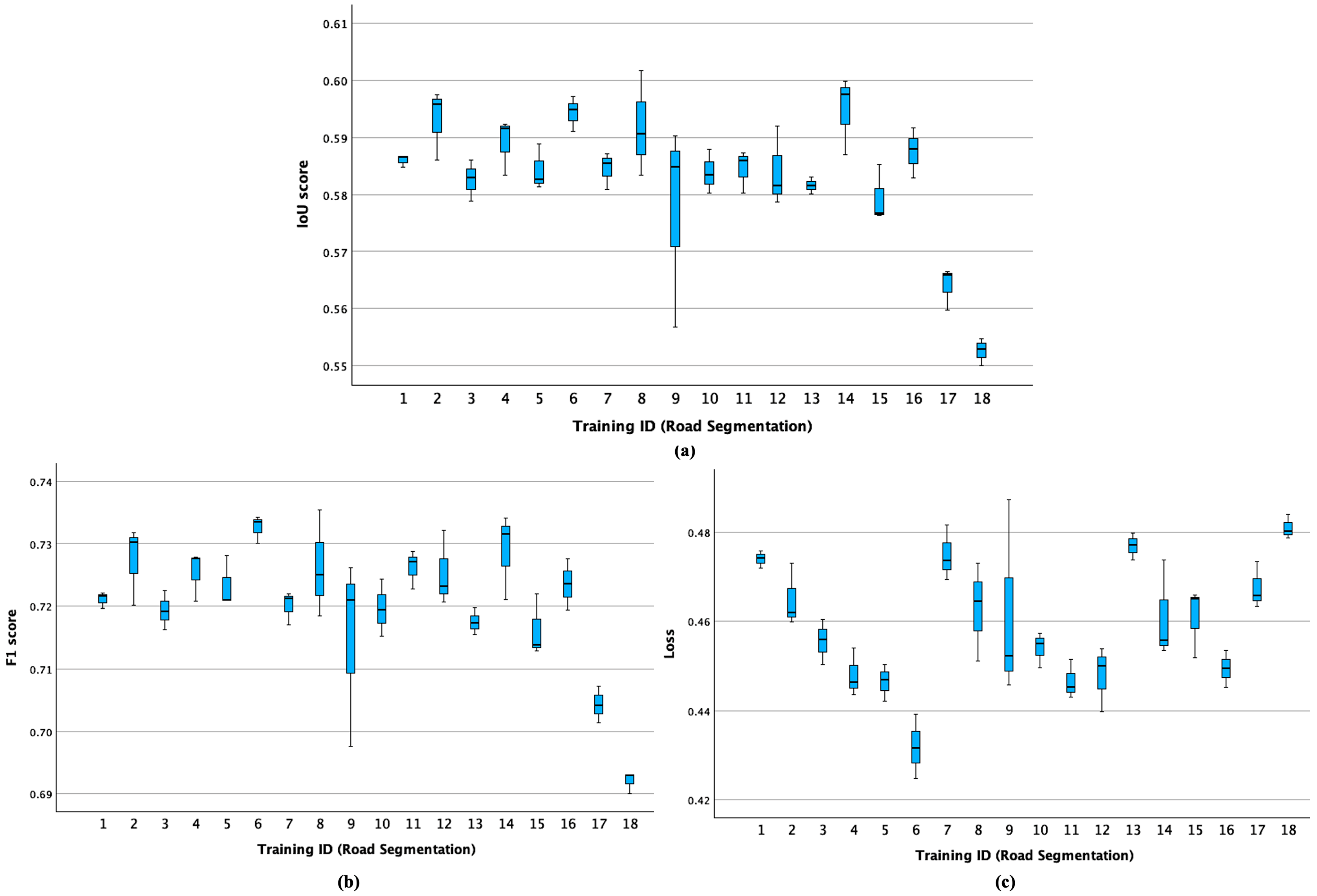
In Figure 2, the boxplots for the performance of the eighteen proposed configurations in terms of IoU score, F1 score, and loss values are presented.

Crossing data from Table 3 with information from Figure 2 (based on the data reported in Appendix A), it appears that the best mean performance on the test set was achieved by the models trained in the scenario with ID = 6 (U-Net—Inception-ResNet-v2, trained on tiles with a size of 1024 × 1024 pixels with 12.5% overlap), which had the highest mean values for IoU Score (0.5943) and F1 Score (0.7326) and the lowest mean value (0.4319). Also, the highest mean IoU score was obtained in the training scenario with ID = 14 (LinkNet—EfficientNet-b5, trained on tiles with a size of 256 × 256 pixels with 12.5% overlap). The models trained on 512 × 512 and 12.5% overlap (training scenarios with IDs = 4, 10, and 16) also appear to achieve consistently high performance across all experiments. The lowest variability in the performance metrics was delivered by the models trained in the scenario with ID = 1 (U-Net—Inception-ResNet-v2 model trained on tiles of 256 × 256 pixels with no overlap).

The worst mean performance is present in the training scenario with ID = 18 (LinkNet—EfficientNet-b5, trained on tiles of 1024 × 1024 pixels with 12.5% overlap), as it presents the lowest mean values for IoU Score (0.5526), F1 Score (0.6920), and the highest loss (0.4809). However, it can also be found that one of the models trained in Scenario 9 (U-Net—SEResNeXt-50 architecture, trained on tiles of 512 × 512 pixels and no overlap) obtained the highest loss (Experiment 25 in Appendix A). The models trained in this scenario (scenario with ID = 9) also featured the highest variability in performance metrics.

As for the lowest variability in performance, it can be found in scenario 1 (U-Net—Inception-ResNet-v2, trained on tiles of 256 × 256 pixels with no overlap), as it has the lowest standard deviations for loss value (0.0020) and IoU Score (0.0011), while the highest one is present in the training scenario with ID = 9 (U-Net—SEResNeXt-50, trained on tiles of 512 × 512 pixels with no overlap), which has the highest standard deviations for the loss (0.0223), IoU score (0.0180), and F1 score (0.0152) values.

6.2. Mean Performance on the Test Data Grouped by Tile Size, Tile Overlap and Semantic Segmentation Model

To further understand these results, the performance metrics on the test set (as dependent variables) were grouped and examined by tile size, overlap, and semantic segmentation model as independent variables (or fixed factors) to determine if the means and standard deviation of metrics are significantly different across the levels of the fixed factors. ANOVA was also applied to inferential statistics (F-statistic and its p-value, together with η and η²). The size of the groups varies from $N=18$ samples for each of the three tile sizes considered to $N=27$ samples for the tile overlap groups and to $N=18$ samples for each semantic segmentation architecture.

In

Table 4. ANOVA analysis of the mean performance metrics across various levels of tile size, overlap, and semantic segmentation architecture.

Independent Variable	Category	Statistical Measure	Loss	IoU Score	F1 Score	Precision	Recall
Tile Size (pixels × pixels)	256	Mean	0.4691	0.5886	0.7235	0.8077	0.6459
		Std. Deviation	0.0091	0.0068	0.0062	0.0040	0.0093
	512	Mean	0.4549	0.5833	0.7199	0.8029	0.6397
		Std. Deviation	0.0102	0.0082	0.0072	0.0053	0.0124
	1024	Mean	0.4536	0.5773	0.7173	0.7687	0.6699
		Std. Deviation	0.0171	0.0151	0.0150	0.0363	0.0218
	Inferential Statistics	F-statistic	8.279	5.054	1.688	17.915	19.164
		p-value	<0.001	0.010	0.195	<0.001	<0.001
		η	0.495	0.407	0.249	0.642	0.655
		η2	0.245	0.165	0.062	0.413	0.429
Tile Overlap (%)	0	Mean	0.4627	0.5805	0.7181	0.7901	0.6513
		Std. Deviation	0.0133	0.0086	0.0078	0.0276	0.0245
	12.5	Mean	0.4557	0.5857	0.7223	0.7960	0.6524
		Std. Deviation	0.0146	0.0134	0.0123	0.0272	0.0147
	Inferential Statistics	F-statistic	3.445	2.904	2.290	0.618	0.042
		p-value	0.069	0.094	0.136	0.435	0.838
		η	0.249	0.230	0.205	0.108	0.029
		η2	0.062	0.053	0.042	0.012	0.001
Semantic Segmentation Model	U-Net—Inception-ResNet-v2	Mean	0.4535	0.5882	0.7249	0.8003	0.6522
		Std. Deviation	0.0146	0.0057	0.0055	0.0123	0.0138
	U-Net—SEResNeXt-50	Mean	0.4580	0.5844	0.7221	0.8024	0.6430
		Std. Deviation	0.0137	0.0088	0.0080	0.0067	0.0144
	LinkNet—EfficientNet-b5	Mean	0.4661	0.5767	0.7138	0.7766	0.6604
		Std. Deviation	0.0121	0.0151	0.0131	0.0411	0.0264
	Inferential Statistics	F-statistic	4.021	5.554	6.768	5.889	3.736
		p-value	0.024	0.007	0.002	0.005	0.031
		η	0.369	0.423	0.458	0.433	0.357
		η2	0.136	0.179	0.210	0.188	0.128

Note: Bold text represents the levels of independent variables with the highest mean performance and significant ANOVA results.

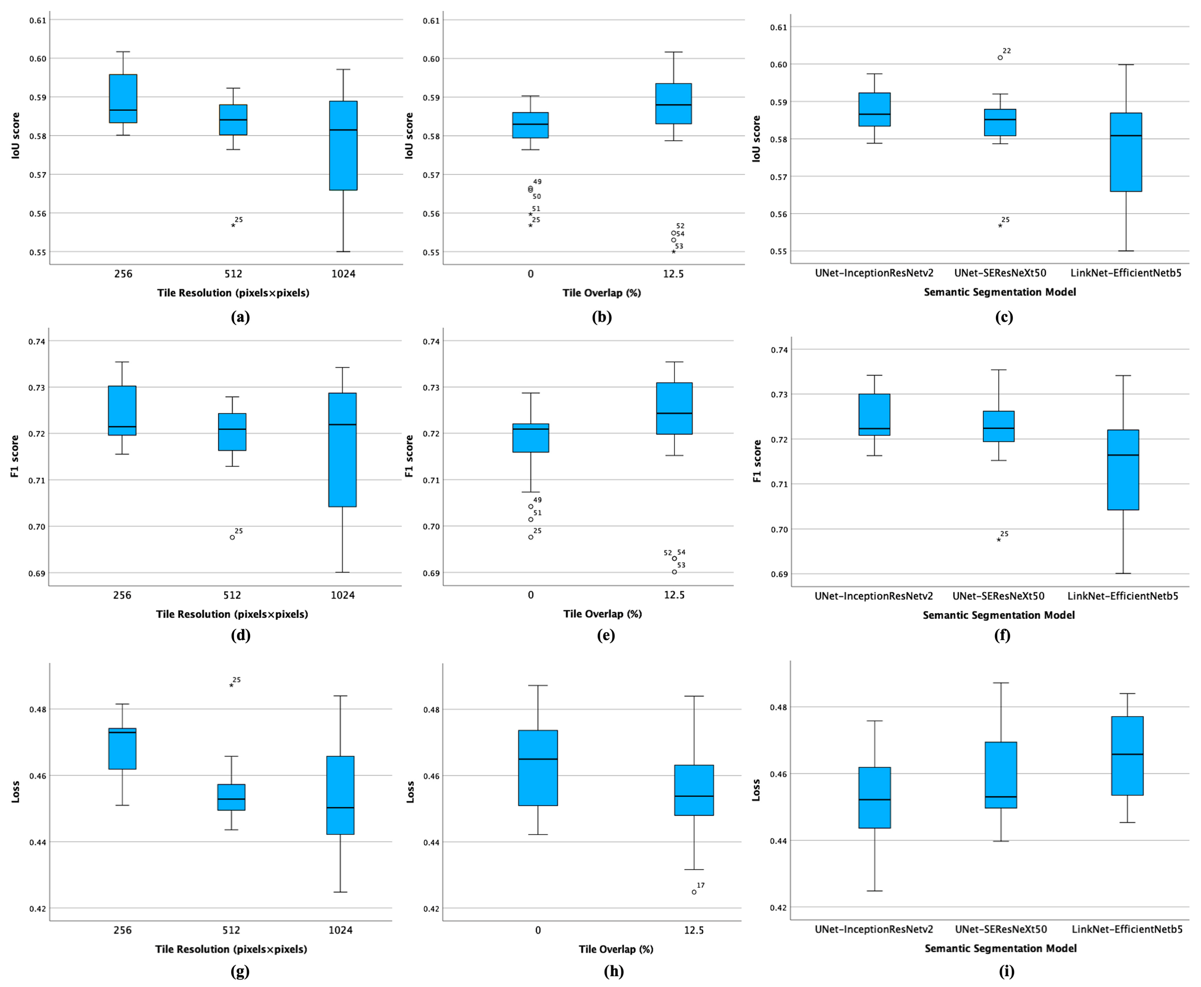
, the mean and standard deviation of performance metrics are presented by the categories of the independent variables “Model”, “Overlap”, and “Size” to explore the relations between these factors. Inferential statistics resulting from the ANOVA table are also provided for further analysis of the differences between the group means and their significance. Figure 3 presents the box plots for the performance grouped by the considered factors.

Values in Table 4 and Figure 3 shows that, in terms of tile size, the models trained on tiles of 256 × 256 pixels achieved the highest mean IoU score of 0.5886 (compared to 0.5833 achieved on 512 × 512 pixel tiles, or 0.5773 achieved on 1024 × 1024 pixel tiles). The largest tile size also featured the highest variability in the IoU metric values, while the models trained on tiles with a size of 512 × 512 pixels achieved the lowest metric variability, except for experiment 25 (an outlier, as observed in Appendix A). This pattern can be observed for the F1 score and loss values.

Crossing these data with information from Table 1, Table 2 and Table 3, it results that the best training setting for the size of 256 × 256 pixels was the training scenario with ID = 14 (LinkNet—EfficientNet-b5 models trained on tiles featuring a 12.5% overlap), as it achieved the highest mean IoU and F1 scores (0.5948 and 0.7289, respectively) and a lower mean loss value of 0.4610 when compared to the rest of the scenarios trained on data with the same size.

The models trained on tiles of 512 × 512 pixels achieved the highest mean values for IoU Score (0.5891) and F1 Score (0.7254) and the lowest mean value for loss (0.4480) in scenario 4 (U-Net—Inception-ResNet-v2 architecture trained on tiles with 12.5% overlap), which has a higher IoU Score (0.5838), lower Loss (0.4540), and higher F1 Score (0.7196) compared to other scenarios with the same size.

Lastly, the models trained on tiles of 1024 × 1024 pixels, in Scenario ID = 6 (U-Net—Inception-ResNet-v2, 12.5% overlap) have the highest mean values for IoU Score (0.5943), and F1 Score (0.7326) and the lowest mean loss value of 0.4319—this scenario achieved the best performance. The differences are statistically significant (p-values of <0.001 and <0.01 for loss and IoU score, respectively), but the mean values of the analyzed metrics are close enough to indicate that a more in-depth evaluation should be carried out (in Section 6.3). The ANOVA analysis shows that the effect of tile size on loss, precision, and recall is significant. This aligns with the observations in Table 3 and indicates that larger tile sizes (1024 × 1024) generally lead to better performance.

Grouping the performance metrics by tile overlap reveals that the segmentation models trained on data with 12.5% overlap consistently outperform (higher median IoU and F1 scores and lower median loss) those trained on data without overlap. As the associated p-value is higher than 0.05, the evidence present in the data is insufficient to reject the null hypothesis (“The mean performances are not different”.) but are close enough to the threshold value to be considered indicative of a trend (p-values of 0.069 and 0.094 for the loss and IoU score, respectively). The ANOVA analysis suggests that the amount of overlap between tiles may not be a critical factor in the mean performance of these semantic segmentation architectures, and further analysis of the effect of tile overlap on the metrics is carried out in Section 6.3. Nonetheless, models trained on tiles with 12.5% overlap result in a lower mean loss of 0.4557 (compared to 0.4627 in the case of “No overlap”), a higher mean IoU score of 0.5857 (versus 0.5805 for “No overlap”), and a higher mean F1 score of 0.7223 (compared to 0.7181 for “No overlap”).

Among the semantic segmentation architectures trained, U-Net—Inception-ResNet-v2 has the highest mean IoU and F1 scores of 0.5882 and 0.7249, respectively, and the lowest mean loss of 0.4535. The best model was U-Net—Inception-ResNet-v2 (with the mean performance reported earlier for the training scenario with ID = 6). The second-best architecture is U-Net—SEResNeXt-50 trained in a scenario with ID = 8 (tiles of 256 × 256 pixels with 12.5% overlap), where it obtained mean IoU and F1 scores of 0.5919 and 0.7263, respectively, and a loss of 0.4628. Finally, the best mean performance of LinkNet—EfficientNet-b5 is present in the training scenario with ID = 14 described earlier (tiles of 256 × 256), featuring a 12.5% overlap. The differences in the model’s performance are statistically significant across all the performance metrics (p-values of 0.024, 0.007, and 0.002 for the loss, IoU, and F1 scores, respectively). The results support the observations from Table 3 and Table 4 and are consistent with those found in similar studies [2].

6.3. Main and Interaction Effects with Factorial ANOVA

Next, to analyze the impact of the independent variables (tile size, or “Size”, tile overlap, or “Overlap” and semantic segmentation architecture, or “Model”) on the performance, factorial ANOVA was applied for the main and interaction effects of the fixed factors on the performance metrics (dependent variables) to explore the effects of one, two or more independent variables (also known as factors) on each metric.

The main effect is the effect of each factor on the dependent variable, while the interaction effect represents the combined effect of two or more factors on the dependent variable (which may differ from the sum of their individual main effects). The null hypothesis of the interaction effect asserts that the effect of one independent variable on the dependent variable remains consistent regardless of the level of another independent variable. Analyzing the interaction effect between two factors reveals whether the relationship between one factor and the dependent variable (performance) changes depending on the level of the other factor. When the p-value < 0.05, the result is deemed statistically significant (it is unlikely that the interaction has occurred by chance), and the null hypothesis is rejected: the performance achieved at a level of the fixed factor does vary at other levels of another independent variable. In this case, it indicates whether the means of the performance are significantly different across the independent variables and whether there are significant interactions between these factors. If the p-value > 0.05, it implies that the evidence present in the data is insufficient to reject the null hypothesis.

Table 5. Main and interaction effects of the size, overlap, and semantic segmentation model (fixed) factors on loss, F1, and ROC-AUC scores (dependent variables).

ID	Source	Dependent Variable	Type III Sum of Squares	df	Mean Square	F	p-Value
1	Corrected Model	IoU score	0.0056 a	17	0.0003	8.257	<0.001
		F1 score	0.0046 b	17	0.0003	8.464	<0.001
		Loss	0.0085 c	17	0.0005	7.678	<0.001
2	Intercept	IoU score	18.3588	1	18.3588	463,213.653	<0.001
		F1 score	28.0115	1	28.0115	879,920.640	<0.001
		Loss	11.3857	1	11.3857	175,315.654	<0.001
3	Model	IoU score	0.0013	2	0.0006	15.772	<0.001
		F1 score	0.0012	2	0.0006	18.865	<0.001
		Loss	0.0015	2	0.0007	11.342	<0.001
4	Size	IoU score	0.0012	2	0.0006	14.586	<0.001
		F1 score	0.0004	2	0.0002	5.583	0.008
		Loss	0.0027	2	0.0013	20.407	<0.001
5	Overlap	IoU score	0.0004	1	0.0004	9.329	0.004
		F1 score	0.0002	1	0.0002	7.587	0.009
		Loss	0.0007	1	0.0007	10.348	0.003
6	Size * Overlap	IoU score	0.0002	2	0.0001	3.036	0.060
		F1 score	0.0002	2	0.0001	3.372	0.045
		Loss	0.0004	2	0.0002	2.814	0.073
7	Model * Size	IoU score	0.0022	4	0.0005	13.658	<0.001
		F1 score	0.0022	4	0.0005	17.186	<0.001
		Loss	0.0027	4	0.0007	10.276	<0.001
8	Model * Overlap	IoU score	0.0001	2	2.5282−5	0.638	0.534
		F1 score	0.0001	2	3.1339−5	0.984	0.383
		Loss	0.0001	2	4.0069−5	0.617	0.545
9	Model * Size * Overlap	IoU score	0.0003	4	8.2644−5	2.085	0.103
		F1 score	0.0003	4	7.9184−5	2.487	0.061
		Loss	0.0006	4	0.0001	2.179	0.091
10	Error	IoU score	0.0014	36	3.9634−5
		F1 score	0.0011	36	3.1834−5
		Loss	0.0023	36	6.4944−5
11	Total	IoU score	18.3658	54
		F1 score	28.0172	54
		Loss	11.3965	54
12	Corrected Total	IoU score	0.0070	53
		F1 score	0.0057	53
		Loss	0.0108	53

Notes: (1) Each source of variation listed in the table is evaluated against the three dependent variables. (2) The adjusted R² values of ^a 0.699, ^b 0.705, and ^c 0.682 represent the variance proportion in the dependent variables that can be predicted from the independent variables by the “Corrected ANOVA Model”. (3) “Total” denotes the total variance in the dependent variables, whereas “Corrected Total” indicates the total variance of the dependent variables after adjusting for the effects of the model. (4) The “Error” row shows the unexplained variance in the dependent variables. (5) The “df” column displays the number of degrees of freedom. (6) The bold text highlights the effects of fixed factors and interactions that have a significant effect on the performance.

reports the statistical results of the “between-subjects” factorial ANOVA test results of the main and interaction effects of the fixed factors mentioned earlier for the three dependent variables (IoU score, F1 score, and Loss performance metrics).

In Table 5, the “Corrected Model” (Source ID = 1) represents the variation explained by the ANOVA model (includes all factors and interactions and indicates the combined effect of all of them). The p-level (<0.001) indicates that the model is statistically significant for the three metrics (IoU score, F1 score, and loss; the dependent variables) and implies that at least one of the factors or their interactions has a significant effect on the dependent variables. “Intercept” refers to the overall mean of the dependent variables—the high F-values and low p-values levels (<0.001) indicate that the overall means of the performance metrics are significantly different from zero.

“Model”, “Size”, “Overlap” (Source IDs 3 to 5) represents the main effects of each fixed factor; all three factors significantly predict the dependent variables, as indicated by the highly significant p-values < 0.001. This indicates that the semantic segmentation model trained and the tile size and overlap levels in the training images significantly impact the performance metrics. It also indicates that future studies should consider the levels of fixed factor performance to optimize the metrics.

The two-way interaction “Size * Overlap” (Source ID = 6) represents the interaction effect between the tile size and tile overlap. The significance level (0.045 for the F1 score) indicates that the interaction between size and overlap significantly affects the F1 score. The p-values of 0.06 and 0.073 for the IoU score and loss, respectively, are not statistically significant but are close enough to the significance level of 0.05 to be considered indicative of a possible trend. As for the interaction effect between the semantic segmentation architecture and tile size (Source ID = 7), the p-value < 0.001 indicates that the interaction between the segmentation model and tile size significantly affects the performance. The two-way interaction “Model * Overlap” (Source ID 8) suggests that the interaction between the semantic segmentation model and tile overlap is not statistically significant (p-value higher than 0.05) and that the interaction between them does not significantly affect the performance metrics—the effect of the semantic architecture does not depend on the level of tile overlap.

The p-values higher than 0.05 of the three-way interaction “Model * Size * Overlap” (Source ID = 9) indicate that the combined effect of the model, tile size, and tile overlap does not significantly impact performance metrics obtained in the road extraction task, beyond their main effects and two-way interactions. However, for the F1 score, the p-value of 0.061 is close enough to the significance threshold to be considered an indicator of a possible trend. Interpreting three-way interactions can be complex, and visualizing the estimated means of the metrics at each level of a fixed factor with the Estimated Marginal Means (EMMs) plots (or profile plots, they are adjusted for the effects of other factors in the model) can be helpful for a better understanding. The EMMs plots for the three-way interaction are based on the data reported in Appendix B and are presented in Figure 4.

For interpreting the plots in Figure 4, the slopes of the lines are important; plotted lines that are not parallel suggest an interaction effect (the steeper the lines, the stronger the effect of the interaction on the dependent variable; parallel lines suggest no interaction). For example, the LinkNet-EfficientNetb5 model trained on tiles of 256 × 256 pixels with no overlap (Figure 4a) has a mean IoU score of 0.5816; this score increases slightly to 0.5948 when there is a 12.5% overlap. A p-value of 0.061 is reported in Table 5 for the three-way interaction (non-significant, but possibly indicative of a trend) on the F1 score, and a more pronounced interaction can be observed in the semantic segmentation models trained on tiles of 1024 × 1024 pixels (Figure 4f), depending on the tile overlap levels (indicated by the crossed lines).

The results described in this section suggest that the performance is significantly influenced by the semantic segmentation architecture trained, the size of the images, and the overlap of the tiles. The interaction between these factors also plays a significant role, especially the two-way interaction between the semantic segmentation model and tile size. The implications are further discussed in Section 8.4.

7. Qualitative Evaluation

To further assess the results of the tests applied in Section 6, a visual comparison of random samples from the test area was conducted using the best models from the scenarios with the highest mean metrics (identified in Section 6.1 and Section 6.2). The objective was to analyze the quality of the predicted road representations delivered by the best models at different tile sizes and verify whether underlying trends can be identified in the correct and false predictions of the models to provide additional insights regarding their prediction behavior.

The predictions delivered by these best semantic segmentation models on random samples from the test set, together with their corresponding orthoimage tile and the ground truth mask, are illustrated in Figure 5. In this section, all comments, insights, and findings related to the extracted road representations refer to the mentioned subplots of Figure 5.

The best model trained on tiles of 256 × 256 pixels was obtained in Experiment 42 of training scenario ID = 14 (LinkNet—EfficientNet-b5, trained on tiles with 12.5% overlap, as found in Appendix A); the model achieved performance metrics of 0.4534, 0.5998, 0.7341, 0.8098, and 0.6639 in terms of loss, IoU and F1 scores, and precision and recall values on the test set, respectively. The best model trained on tiles of 512 × 512 pixels was obtained in Experiment 11 of training scenario ID = 4 (U-Net—Inception-ResNet-v2, trained on tiles with 12.5% overlap, as found in Appendix A); the model achieved performance metrics of 0.4465, 0.5923, 0.7276, 0.8118, and 0.6444 for the loss, IoU and F1 scores, and precision and recall values on the test set, respectively. Finally, the best model trained on tiles of 1024 × 1024 pixels was obtained in experiment 17 of training scenario ID = 6 (U-Net—Inception-ResNet-v2, trained on tiles with 12.5% overlap, as found in Appendix A); the model achieved performance metrics of 0.4248, 0.5948, 0.7335, 0.8030, and 0.6594 for the loss, IoU and F1 scores, and precision and recall values on the test set, respectively.

7.1. General Trends

In the visual comparison between the aerial tiles, ground truth masks, and model predictions, it was observed that, in general, the road representations in the predictions are a clear improvement over the ground truth masks. This improvement occurs in three main aspects: (1) streets, paths, and/or other roads present in the aerial imagery but not present in the segmentation mask (for example, the upper part of Figure 5(f2)) are extracted by the models; (2) the geometries of the road representation and the logic of their layout (for example, at their intersections) are also clearly improved with respect to the ground truth masks (as seen in Figure 5(c3)); and (3) the real width of roads is reflected in the predictions (for example, comparing Figure 5(b6) and Figure 5(c6)).

Regarding the identification of new roads, these are not always extracted in a clearly defined way but with some degree of uncertainty (predicted probabilities closer to 0.5). This can be observed in the upper left of Figure 5(f1) or in Figure 5(f3) (road representations without continuity), but it is important to note that remotely sensed scenes where this scenario is encountered are usually complex and present obstructions that would make extraction difficult for humans as well.

It should also be noted that the extraction of new roads is found in all three tile sizes considered. The improvement is also observed in the geometric layout predicted since the roads are represented with smoother curves and closer to reality than in the ground truth masks, as illustrated in Figure 5(a2,b2,c6). Another improvement in the drawing is the identification of cut streets (cul-de-sac), frequent in residential areas, as observed in Figure 5(f2) (bottom right part, where an alley that is not connected to the highway is correctly extracted by the model, despite not being reflected in the ground truth mask).

This incorporation of new elements and connections helps to improve the logic of the road layout. For example, by comparing the lower central parts of the segmentation mask and the predicted mask from Figure 5(e3,f3), respectively, it can be observed that the ground mask does not contain any road representation in the residential area. A similar case can be observed in the lower right part of Figure 5(i3). Another example is shown in Figure 5(i1), where urban houses are better connected to road exits when compared to Figure 5(g1). Nonetheless, predictions from tight urban layouts should be improved with post-processing. Another example of improvement is observed in the upper rectangle of Figure 5(f3), where connecting sections that are hidden by vegetation are correctly connected, unlike in the segmentation mask from Figure 5(e3), where the road parts are disconnected.

Furthermore, an improvement in the representation of the true road widths is widely observed in the predicted masks. For example, in Figure 5(a6,b6,c6), the differences in road widths are evident; the predictions from Figure 5(c6) better reflect the true road widths when compared to the masks from Figure 5(b6). Another example can be seen in Figure 5(d1,e1,f1), where Figure 5(f1) better illustrates the difference in amplitude of the main road from the aerial tile of Figure 5(d1) when compared to the ground truth mask from (e1).

Another pattern observed is related to a better extraction of road information near bridges and underpasses. For example, although in the lower central part of the predicted mask from Figure 5(i3), it initially might appear that there is a problem with disconnected road segments, it is an underpass that is missing from the ground truth mask from Figure 5(g3). This can also be observed in Figure 5(d5,f5). Furthermore, in the official ground truth masks, the representation of road bridges over highways seems to intersect with the highways, although the drivable area of a bridge and overpass is beneath or over a highway. It is proposed to train a model that detects these structures and decides a better approach for representing these road regions.

Small prediction artifacts near the image borders are still present even in the best models (in the form of thickened road representation (for example, in Figure 5(f1)), or missing road pixels at the very edge of the prediction mask (for example, in the upper central part of Figure 5(i1)). In addition, there are some unexpected prediction errors, such as the obvious missing road segment observed in the lower central part of Figure 5(i3).

7.2. Areas with Higher Error Rates

In general, road elements present more differences from the ground truth in scenes with road widening, like when small spaces or squares are formed (for example, in Figure 5(c9), the central rectangle of Figure 5(c10), or in Figure 5(i1)). These differences also occur in regions with very short segments of road, such as the incorporation marked in the bottom right of Figure 5(f1). The errors associated with wider roads are more accentuated when they occur near tile edges, where the identification becomes blurred and loses sharpness (for example, the upper central part of Figure 5(c7), the lower central part of Figure 5(i2), or in the upper left rectangle of Figure 5(f4)). However, this effect seems to be attenuated in medium-sized tiles; for example, the road to the north of the roundabout in Figure 5(f2) has a higher quality. The part corresponding to the lower center of Figure 5(g3) results in an omitted road representation in the prediction mask. Therefore, wider roads can be considered as a significant conditioning factor in urban scenes (caused by public squares or street openings).

There is also qualitative evidence that road extraction problems near the tile edge of the image are caused by the angle of incidence of the road with the edge. For example, the road part from the upper left corner of Figure 5(d5) was not predicted in Figure 5(f5). Another example is the widening at the central edge in Figure 5(d6), which causes issues in the prediction mask in Figure 5(f6). The same case is illustrated in the upper parts of Figure 5(c3,i1), where wider roads with shorter lengths are present near the tile border. These errors near the edges can also be observed on the upper left side (near the roundabout) of Figure 5(c2) or in the intersection of the road and roundabout at the central left part of the subplot of Figure 5(c4). Otherwise, a sufficient road length enables the correct identification of the event at the edges of the image (as found in Figure 5(c8,f5,i1)). Therefore, the existence of short stretches of roads that touch the edge of the tile at a considerable angle appears to result in higher prediction rates.

7.3. Observed Behavior in Rural and Urban Scenes

The prediction behavior observed in rural and urban scenes shows different patterns, although they are related to differences in contrast in the aerial image. In urban areas, the biggest error sources are the shadows of buildings, which cause significant differences in contrast, while in rural areas, tree occlusions produce higher rates of errors.

In urban areas, the problem of shadows in narrow streets, which confuse the models, is detected. This can be observed in the lower left rectangle of Figure 5(f4), where the shadows of the buildings obstruct the correct prediction of the road. The same occurs in the other green-marked rectangle, where shadows impede the clean extraction of the roads. Nonetheless, it is important to note that these sections were not identified in the mask but were in the prediction mask. Other examples are indicated with green rectangles in Figure 5(c7), where the DL model correctly extracted a road that was not present in the official road cartography. Note the negative impact of inaccurate ground truth masks on the IoU scores in tiles where correct predictions are labeled as “false positives” due to errors in the available cartography.

These problems are more pronounced in models trained with tiles of 256 × 256 pixels and appear to affect less the models trained with larger tiles. For example, the shadow of the street in the central area marked in green in Figure 5(d1) occupies the entire road but does not prevent its correct extraction; the same occurs with the shadow of the building near the lower left corner in Figure 5(d4).

In urban scenes like central squares of older towns, where the connectivity of the roads is more complex due to the larger paved surfaces and the spectral similarities of the surrounding environment, the models achieved lower IoU scores (for example, in Figure 5(c9)). This was also observed in scenes where pedestrian lanes feature similar spectral similarities to the road pavement (for example, worn road pavement that was not renewed and changed color, as in Figure 5(c10) or Figure 5(i1)). It can also be noticed that in older urban environments, where the identification of roads can become difficult even for humans, the representations extracted by the models are superior to those available in the ground truth masks, where the road representations are often not aligned with the corresponding aerial imagery. For example, in Figure 5(c1,c9,c10), or Figure 5(f1,f6), the intersection of public squares with nearby streets is better represented.

Furthermore, streets that are present in the aerial images but not in the ground truth mask were successfully extracted by the models, especially at larger tile sizes (such examples of streets can be found in Figure 5(i1,i3) or Figure 5(f1,f6)). Again, note the impact of these true road predictions that are absent from the ground truth mask; they lower the IoU scores achieved by the model in those scenes.

Rural areas present problems caused by the significantly different spectral signatures of pavement materials, and models sometimes fail to extract longer road sections. An example of this is evident in the central green rectangle in Figure 5(d4), where the unpaved road leading to the isolated house has not been identified because it is almost indistinguishable from the background at the intersection with the main road. Other examples are the suggested path from the top left part of Figure 5(f1), which is not suitable for vehicles, or the trodden path in the upper left corner of the image of Figure 5(i1). For a cleaner road layout, it is recommended that these ambiguous predictions be removed using rule-based post-processing.

Tree occlusions in rural areas seem to be well resolved when the contrast conditions are favorable, and they do not cause large interruptions in the road layout. Such examples can be found in the upper central part of Figure 5(f3) or near the road indicated in the lower left of Figure 5(h2) (where many tree occlusions are present). In both cases, significant differences in contrast between the road material and the vegetation are significant. However, in the same green rectangle in the lower left of Figure 5(h2), the identification of the unpaved road that runs from North to South (parallel with the main road), where less contrast is present, was omitted.

Another drawback identified in more rural areas is related to the extraction errors of the changes between roads and unpaved roads or paths. For example, in the central part of Figure 5(f6), the change between the paved and unpaved roads is not signaled but is extracted as the continuity of the road. Another instance is illustrated in the lower right part of Figure 5(c8), where the road-path intersection presents a high degree of uncertainty in the predicted layout (tree obstruction could also be a contributing factor).

7.4. Tile Size with Best Predictions and Other Considerations

In the qualitative analysis, it was found that although the road representations resulting from the semantic segmentation are closer to reality when compared to those provided as ground truth, this might sometimes heavily impact the IoU scores (for example, in Figure 5(c4)). Nonetheless, the quality of the geometric representations of the predictions is particularly evident at traffic roundabouts and road junctions (as illustrated in Figure 5(c2), Figure 5(f2), or Figure 5(i2)). Lane separation from highways seems to be closer to reality (as shown in the upper left corner of Figure 5(i2)).

The visual interpretation showed that models trained at higher resolutions delivered better results. In this regard, it was observed that models trained on tiles of 256 × 256 pixels had larger areas of uncertainty and generally worse predicted road representations. For example, in the predicted masks from the column with the predictions of models trained with tile sizes of 256 × 256 pixels (column “c” in Figure 5), significant areas of uncertainty are presented (although to a lesser degree in Figure 5(c6,c7,c8)).

This occurrence of uncertainties seems to decrease in the medium images and larger images. The visual, qualitative comparison of the medium and large images indicated that training on tiles of 512 × 512 pixels delivered the best road representations and road layout, together with a better geometry of the road structures, particularly in urban areas. An example can be observed in the common area in Figure 5(c2,f2,i2) (close to the roundabout present in the three predicted masks). In upper central Figure 5(f2), the NE-SW road that connects the main road with residential urbanization (not seen in the ground truth mask) is clearly predicted but only hinted at in Figure 5(i2,c2).

Other examples of better predictions of the best model trained on tiles of 512 × 512 pixels can be seen in the common areas of Figure 5(f2,i2), near the alley (cul-de-sac), represented with an inclined rectangle in the lower right part of Figure 5(f2), or the link between this alley and the main round found SW of the medium image, which are not extracted in the largest tile size.

Another representative example is the layout of roads in pairs from Figure 5(f5) and Figure 5(i3) (in the common regions near the area marked with inclined rectangles in both tiles). It can be observed that the road layout extracted in Figure 5(f5) is much closer to reality and does not feature a significant omission of evident roads (unlike the predictions from Figure 5(i3)). Another evident difference is that the best model trained on tiles of 1024 × 1024 pixels does not correctly extract the higher underpass entrance (lower central part of Figure 5(i3)), while the best model trained on the tile size of 512 × 512 pixels does (lower left part of Figure 5(f3)). Another significant improvement within the same pair of prediction masks can be found in the residential area, where roads not featured in the ground truth masks were extracted by both models, but their representation is better in the medium tile size (upper right part of Figure 5(f5)) when compared to the road representations present in the largest tile size (central right part of Figure 5(i3)). Nonetheless, the models trained on 1024 × 1024 pixels also feature high-quality predicted road features, and their mean performance metrics proved to be the highest in Section 5, but also with higher metric variability.

8. Discussion

In this work, the effects of tile size and overlap on semantic segmentation architectures trained for road surface area extraction on a large-scale dataset were studied in a quantitative and qualitative manner on the test, unseen data to assess the significance of the computed performance metrics. The task of supervised extraction of pixels belonging to the road surface areas from an orthoimage is complex due to the natural underrepresentation of the positive class and the challenges associated with remotely sensed data and DL algorithms. As shown in Table 2, the percentage of road pixels of the data used for semantic segmentation is reduced and varies from around 2.5% to 5% of the total number of pixels in an aerial tile, with higher tile sizes containing a lower percentage). This aspect required adaptations in the training methodology presented in Section 5 to ensure model convergence.

8.1. On the Mean Performance

The use of a substantial dataset proved beneficial for DL models, as high and consistent performance was observed across the training, validation, and test sets (Appendix A). This indicates well-fitted models and the absence of underfitting (signaled by low performance on the training set) or overfitting (signaled by high performance on training and low performance on unseen data). As expected, the performance is slightly higher on the training set and lower on the validation and test sets, and there are differences in performance within and across the training scenarios considered. For this reason, in Section 6.1, ANOVA was applied to determine if the mean performance metrics are significantly different across different training scenarios and to examine how they change.

High mean values of the loss, IoU score, F1 score, precision, and recall metrics were observed, with some degree of variability in the performance, as indicated by the standard deviation in the performance. As for the trade-off between precision and recall, in the context of binary semantic segmentation of road surface areas (where the positive class occupies around 3% of an image), it can be interpreted as follows. A higher precision indicates a model that has higher accuracy in predicting whether a pixel is part of the road, at the cost of missing some road pixels (leading to a lower recall, the most common scenario found in Table 2), while a higher recall indicates a model that is better at correctly identifying a large proportion of road pixels, at the cost of incorrectly classifying some background pixels as the road (leading to a lower precision). Models trained on tiles with sizes of 1024 × 1024 pixels and 12.5% overlap achieved the best mean results (training scenario with ID = 6), suggesting that a larger tile size and overlap can improve performance.

The η and η² measures from Table 3 indicate a strong positive association between the performance metrics means and the Training ID levels. The differences in mean performance are highly statistically significant (p-values < 0.001) for all performance metrics considered and prove that the training set has a significant impact on mean performance.

Additional insights were obtained by analyzing the mean performance grouped by tile size, overlap, and semantic segmentation models. First, it was observed that the tile size level has a significant impact on mean loss, IoU Score, and precision and recall metrics (p-values < 0.05). The boxplots in Figure 3 show how lower resolutions can achieve higher median IoU results but also higher median losses, while the models trained on tiles of 512 × 512 pixels achieved the most stable performance. Crossing this with data from Table 4 indicates that it might be caused by the lower performance achieved by scenarios with IDs 17 and 18. It is interesting to note that the best and worst performing models both use a 1024 × 1024 size and 12.5% overlap but with different deep learning models (U-Net—Inception-ResNet-v2 vs. LinkNet—EfficientNet-b5). This suggests that the choice of deep learning model can have a significant impact on performance, even at the same levels of tile size and tile overlap.

This analysis of the mean performance also suggested that a tile overlap of 12.5% can improve the mean performance of the models compared to those trained on tile data without overlap (with non-significant p-values for loss and IoU scores that are close enough to the significance threshold limit to indicate a possible trend). Figure 3 shows that this is consistent across all three models and all three sizes and indicates that a more tile border context might help a model make more accurate predictions.

The model architecture chosen significantly impacts the mean performance achieved, with significant p-values being computed across all dependent variables. When comparing the three architectures, it appears that the U-Net—Inception-ResNet-v2 model consistently outperformed the mean performance of the other models across different sizes and overlaps; the performance improves as the size increases from 256 × 256 to 1024 × 1024, suggesting that higher image pixel counts (more scene information) generally lead to better performance.

This time, the η and η² measures of association from Table 4 indicate a weak positive association between the performance metric means considered and the different levels of the fixed factors. The performance boxplots in Figure 2 and Figure 3 are aligned with the results in Table 3 and Table 4 and support these considerations.

8.2. On the Main and Interaction Effects

Factorial ANOVA was used to quantify the main and interaction effects of the fixed factors “Tile size”, “Tile Overlap”, and “Semantic Segmentation Model” on the performance. The results are presented in Table 5 and analyzed in Section 6.3.

The results prove that the individual effects of tile size, overlap, and semantic segmentation model (main effect hypothesis) on the performance achieved on unseen data are statistically significant. The p-values indicate that the size of the images used for training had a significant impact on the performance and the mean performance analysis and suggest that tiles of larger size might improve the model’s ability to accurately segment the road surface area. Furthermore, the results show that the effect size of tile overlap on the dependent variables is statistically significant (affects the performance; the performance changes at different levels of overlap, although mean differences from Table 4 were not statistically significant) and indicates that providing additional border context to the tiles enables more accurate predictions and suggest that including a small degree of overlap between training image data might be beneficial for the model. The results also indicate that the choice of the model significantly affects the prediction performance and that it is beneficial to experiment with different semantic segmentation architectures and to identify and select the one that provides the best predictions.

As for the two-way interaction effects, the interaction between the semantic segmentation model and tile size (“Model * Size”—source ID = 7) significantly affected performance, suggesting that the optimal size might depend on the specific model used. This means that the effect of the semantic segmentation model on the performance changes depending on the tile size, and vice versa (i.e., one model might perform better than another at a certain tile size but worse at a different tile size, also indicated by the difference in performance between models from training scenarios ID = 5, 6, and 17, 18). Therefore, when experimenting with different models, it should also be considered how the model performance changes at different tile sizes. The p-values were highly statistically significant (p < 0.001) for each dependent variable.

For the “Size * Overlap” interaction (source ID = 6), the p-value indicates the effect of tile size on the F1 score is not constant but depends on the level of overlap, and vice versa (increasing the tile size might improve the F1 score at a certain level of overlap, but not at another). The p-values (between 0.045 and 0.073) are only significant for the F1 score but close enough to 0.05 to be considered indicative of a trend. Finally, the two-way interaction “Model * Overlap” (source ID = 8) indicates that the effect of the model used on the dependent variables is not dependent on the level of overlap, and vice versa (p-values are not significant), so these factors could be considered independently, following the recommendations commented previously.

The three-way interaction effect among fixed factors (source ID = 9) presents p-values that are non-significant and suggests that the combined effect of model, size, and overlap is not significantly different from the expected individual and two-way interaction effects. In other words, the interaction between the fixed factors does not appear to significantly predict the performance metrics (p-values between 0.061 (F1 score) and 0.103 (loss) are higher than the threshold of 0.05 for all the dependent variables, but close enough to it in the case of F1 score to be considered a possible indicator of a trend) and could suggest that, while the choice of model and size is crucial for optimal performance, the effect of overlap is less pronounced and does not significantly interact with the model choice (the effect of the model does not seem to depend on the level of overlap or the combination of tile size and tile overlap). These considerations are reinforced by the EMMs plots in Figure 4.

In conclusion, the main effect of the model, size, and overlap, and their interactions have varying degrees of impact on performance. The main effects are significant for each performance metric. In Table 5, sources with IDs 6 to 9 represent the effects of two-way and three-way interactions between the fixed factors. The “Size” and “Overlap” interaction is significant in the case of the F1 score (p-value of 0.045). The two-way interaction “Model * Size” is significant for all three dependent variables (p-value < 0.001). The other interactions are not significant but often close enough to the significance threshold value of 0.05 for the F1 score (values close to the significance threshold are considered indicators of a possible trend). These insights can be valuable for further optimization of semantic segmentation tasks and can provide guidance for achieving optimal DL performance.

8.3. On the Qualitative Evaluation

Visual comparison of the predictions on the test set delivered by the best models trained at each tile size demonstrated that qualitative, non-numeric evaluations can help identify trends and patterns more easily. The qualitative evaluation carried out reinforced the quantitative analysis, showing that the models trained on larger tile sizes (512 ×512 or 1024 × 1024 pixels) and 12.5% overlap delivered higher-quality predictions compared to those trained on smaller tile sizes with the same overlap level. This suggests that the additional scene information is beneficial for DL models trained for road extraction with semantic segmentation, enabling them to achieve higher performance and generalization capability. In this regard, when comparing common areas in different image sizes, it was observed that the models trained on medium images delivered the highest-quality road representations and best road layout interpretation.

The sources of uncertainty that affect predictions differ between rural and urban scenes. It was observed that the models performed worse in urban areas despite there being sufficient training data in both cases. This could be attributed to the increased layout complexity in urban areas (road widening near public squares) compared to a rural environment where the roads are bordered by geospatial elements with different spectral signatures, for example, green vegetation. The decrease in the contrast between pavements in urban areas or the shadows in narrow streets also worsened the predictions, while in rural areas, vegetation obstructions affected most of the performance. In rural areas, there were also problems in the identification of transitions and intersections between secondary unpaved roads and main roads.

Another interesting insight was that although DL models extracted more secondary roads, the representations were not of high quality. This may have been caused by the lack of representation in the training set. Although these roads may be less important, as they host less traffic, autonomous vehicles should be provided with as much open road cartography as possible to increase road safety.

The patterns observed suggest that it is recommended to follow the multi-approach extraction perspective by isolating urban and rural data from the SROADEX dataset and using it to train different models specialized in extracting roads from urban and rural scenes. Furthermore, extracting the marked representative road lines can also help with lane division, as a rule-based inference from the extracted road surface areas would be more challenging and less accurate.

Another generalized problem was the predicted road representations near bridges (roads that appear to overlap in aerial imagery but are found at distinct heights on the terrain). This might be addressed with the implementation of a DL model specializing in the detection of bridges and the inclusion of a human operator in the extraction process (to manually digitize complex areas). Short road segmentation found near the edge of a tile also seems to cause higher error rates and is often not extracted.

It was also observed that the training dataset (containing the ground truth, based on official road cartography) includes representations that do not cover the entire road surface area from the orthophotos, and this had a direct impact on the computed Intersection over Union (IoU) scores. In any case, a visual comparison of the images, their ground truth masks, and predictions indicate that the three networks generalize well, as the geometric shapes found in the predictions align with the expected results. The predicted roads significantly improved in three aspects: (1) extraction of roads that were not present in the ground truth mask set, (2) improved geometry of the road and in the logic of their connection and layout, and (3) a better representation of the road widths.

8.4. On the Uncertainty of the Models, Limitations of the Study, and Future Directions

The task of binary semantic segmentation of road surface areas from aerial imagery is inherently complex due to the nature of the geospatial object studied and the challenges associated with remote sensing data. Another significant source of uncertainty can be considered the ground truth masks, as the road representations were labeled in vector format, and the conversion to raster is not error-free. These factors are important sources of uncertainty that cannot be removed, but their effects can be reduced using a diverse and representative training dataset based on high-resolution, publicly available aerial imagery (described in Section 4).

The training process can also be considered a source of uncertainty. To address this source of uncertainty, the training of the DL models featured the same training hyperparameters for all experiments. The training process nonetheless has a convergence randomness associated with it, and for this reason, three experiments were run for each training set. There is room for improvement as a higher number of experiment repetitions would enable a more reliable statistical analysis, but considering that the experiments required more repetitions would result in unfeasible training times on the available computational budget. A future study could run more repetitions (for example, ten) to increase the statistical significance of the results. More related aspects are commented in the “Discussion” section of [4].

The insights highlight the importance of selecting the data used for training DL models, and these findings can be applied in several practical ways in real-world scenarios, particularly in the field of geo-computer vision for geospatial object extraction. It is recommended that these findings be further assessed and be further validated with empirical studies to optimize the settings for different models and tasks. For example, a future study could consider more segmentation model architectures and levels of tile size and tile overlap, but it should be noted that the number of training experiments would grow exponentially.

In addition, there is always the possibility that the effect could be caused by other factors that were not considered in this study; however, the use of a large-scale dataset (representative as diverse), as well as the application of the same hyperparameter settings for all experiments, allowed us to address this source of uncertainty. Statistical interpretations should be used as part of a broader analysis, as the observed differences in performance could still be meaningful in a practical sense, especially if the improvements lead to better performance on specific tasks. For this reason, a qualitative evaluation of the best models was carried out. It was observed that images of larger size deliver better results but also require more computational resources, and this trade-off should be considered depending on the computational budget available.

Finally, these observations are based on the road data used in this analysis and may not be applicable to all geospatial object extraction tasks. Nonetheless, these insights could be valuable and can guide future research and practical applications—based on this analysis; it is recommended that future works use data with a small percentage of overlap and test different combinations of model and tile sizes to achieve the best extraction performance in the context specific to the application tackled.

9. Conclusions

In this study, the impact of tile size and tile overlap on the performance of DL models trained for road surface area extraction from aerial imagery with semantic segmentation was statistically analyzed, and further insights on the effects of the levels of fixed factors on model performance were provided. Real-world data covering large regions of the Spanish territory were used to train and test the DL implementations.

The statistical analysis carried out showed that overlap between neighboring tiles (more context for border regions of an image) could improve the performance of these models across all training scenarios, with a higher performance on unseen data being achieved by models trained on datasets featuring a 12.5% tile overlap. The mean performance analysis also showed that additional scene information can result in more robust road extraction models, as larger tile sizes seem to maximize the performance on unseen data. The best mean test IoU score of 0.5943 was achieved by U-Net—Inception-ResNet-v2 trained with tiles of 1024 × 1024 pixels with a 12.5% overlap in Scenario ID = 6.

The main and interaction effects tests showed that the impact of tile overlap, tile size, and semantic segmentation models is statistically significant, with each independent factor having a considerable impact on the performance achieved by the models. The p-values were also significant for the two-way interaction between tile size and tile overlap and between tile size and DL architecture (highly significant p-values < 0.001).

The qualitative visual analysis carried out post-training with the best models from each tile size also indicated that the results with the highest quality were delivered by the DL model trained on image tiles of 512 × 512 and 1024 × 1024 pixels with a 12.5% overlap. These combinations are recommended for future studies. The patterns observed in the qualitative analysis suggest that a multi-perspective approach for road extraction, where several DL models are applied within a common environment built to create a reliable road decision support system, might be beneficial. In this way, the system would include various models specialized in extracting roads from rural or urban areas, in detecting bridges to maximize the quality of the representations. In more complex extraction scenarios, the involvement of the human factor should be considered.

Based on the findings from this work, for future studies, it is recommended to use data with a small overlap and try different combinations of different semantic segmentation models and tile resolutions during training to identify the most suitable one for the approached task. The optimal combination of these two factors, i.e., that achieves the highest metrics, can vary, and it may depend on the specific tasks and DL models used. These insights can guide the development and optimization of semantic segmentation models in various applications, such as autonomous driving, where accurate road extraction is fundamental, or provide for additional geospatial element extraction workflow. In addition, at the highway level, it might be more interesting to extract information related to representative road lines, as there is an abundance of traffic signaling for traffic guidance that can be found at the pavement level.

In future works, it is proposed to identify the optimal combinations of the factors that proved to be statistically significant and provide more nuanced strategies for model development (for example, tailoring the size based on the specific model used). Also, more research with additional models and a higher number of experiment iterations could be conducted to provide more statistical significance to the results and further understand the impact on performance (a considerable computational budget would be required, as the introduction of additional levels of a factor exponentially increases the number of required experiments). Finally, it would be interesting to explore the impact and interactions of the spatial, spectral, or temporal resolutions on the performance of DL models used in geo-computer vision works.