
Estimating Forest Inventory Information for the Talladega National Forest Using Airborne Laser Scanning Systems

 ,
,  , ,
, ,  ,
, 
Abstract
:1. Introduction
2. Materials and Methods
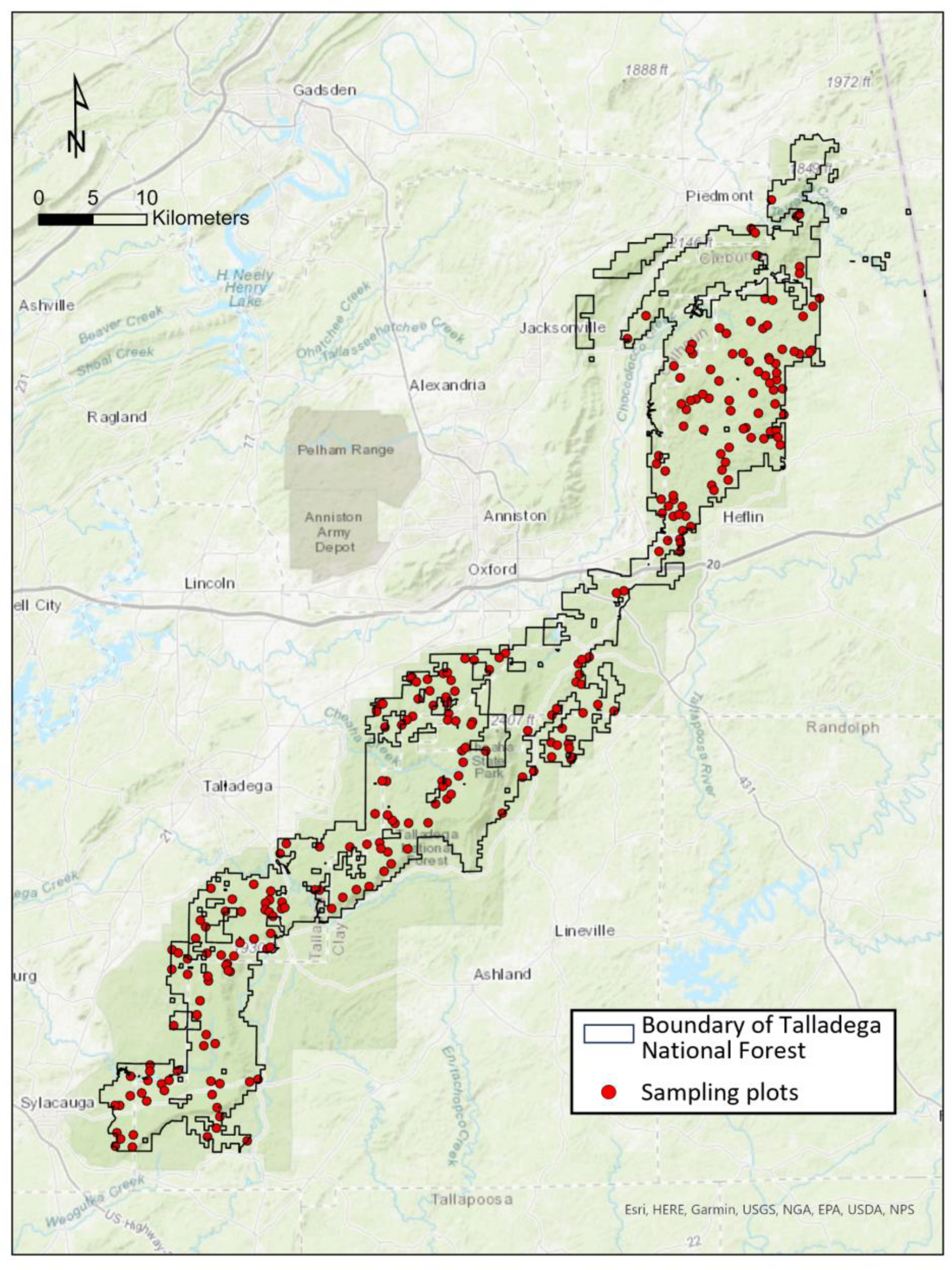
2.1. Study Area
2.2. Data Collection
2.2.1. Field Data Collection
2.2.2. Remote Data Collection
2.3. Data Processing
2.3.1. Field Data Processing
2.3.2. Remote Data Processing
2.4. Modeling
3. Results
3.1. Field-Based Forest Inventory
3.2. Regression Models
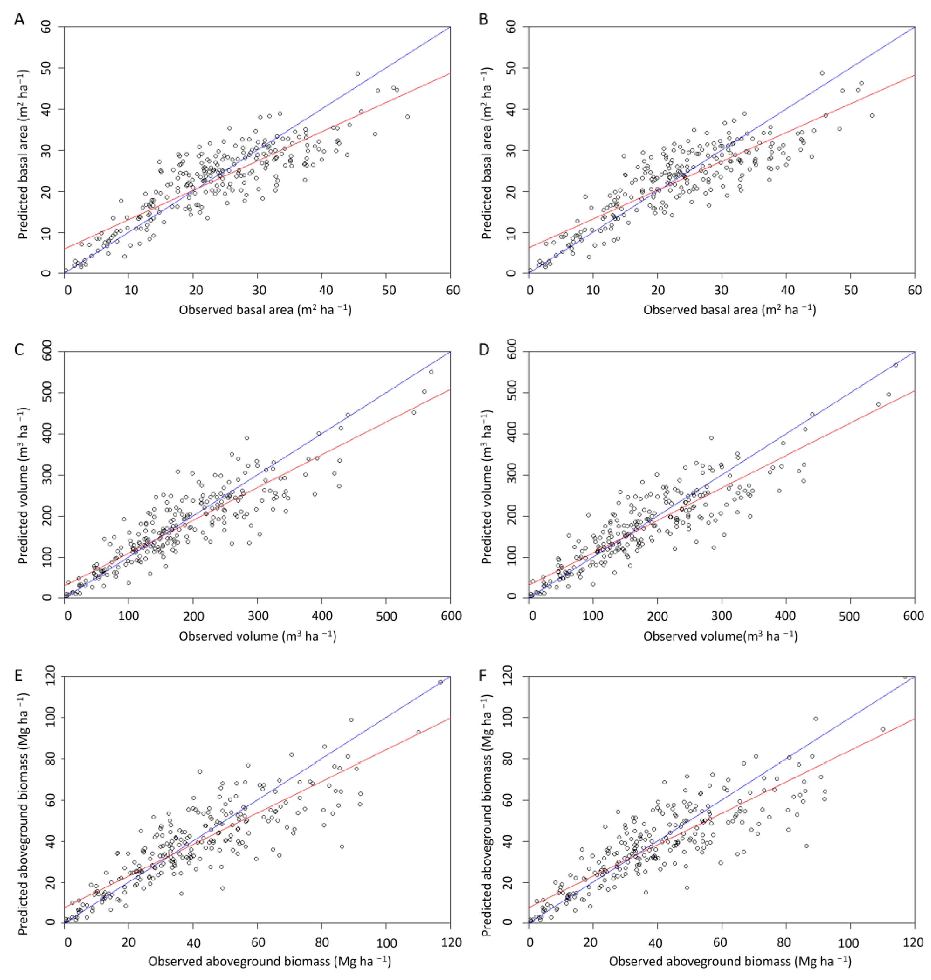
3.2.1. Estimation of Forest Attributes Based on General Models
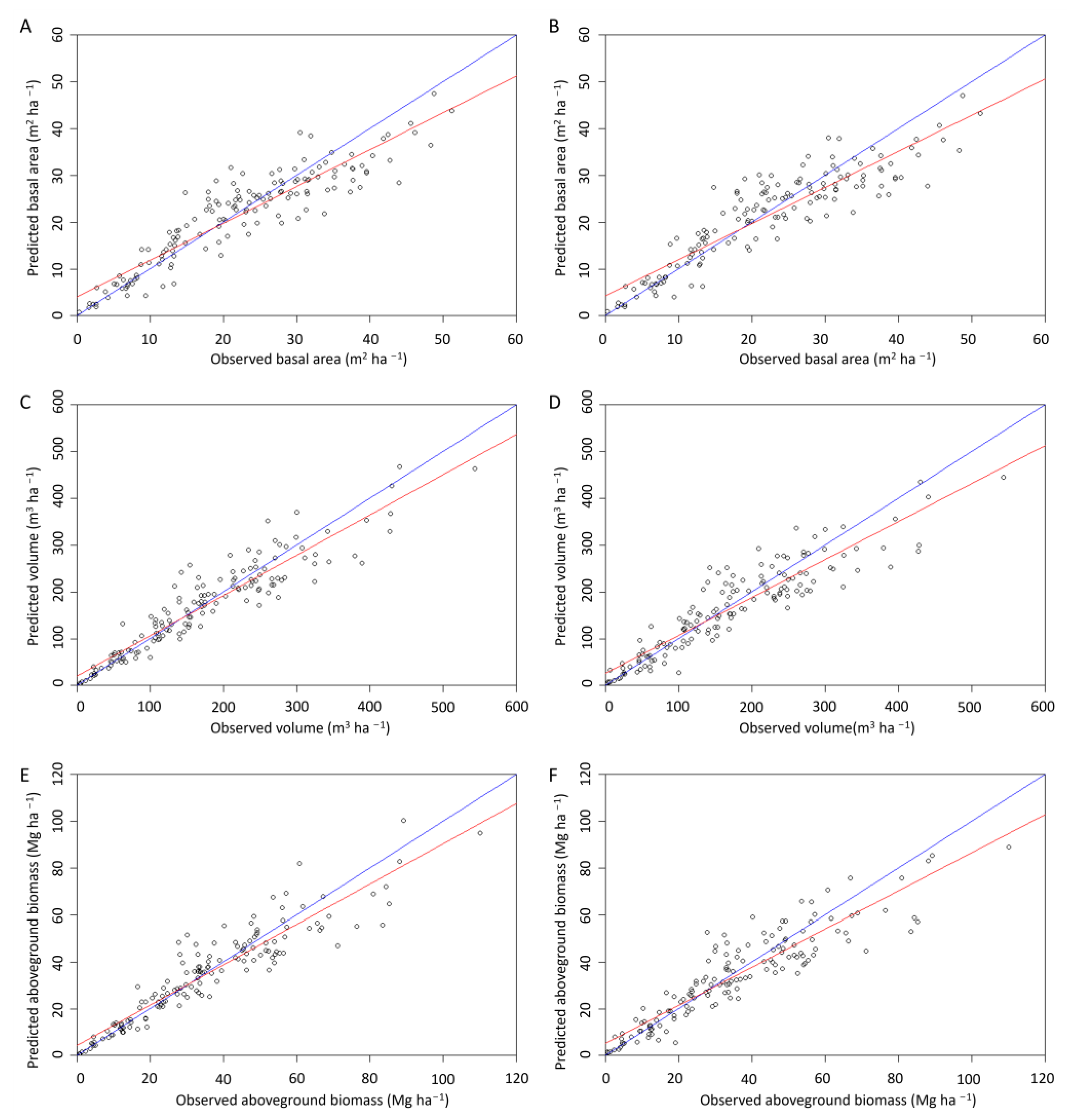
3.2.2. Estimation of Forest Attributes Based on Pine Models
4. Discussion
5. Conclusions
Supplementary Materials
Author Contributions
Funding
Data Availability Statement
Conflicts of Interest
References
- Bettinger, P.; Boston, K.; Siry, J.P.; Grebner, D.L. Forest Management and Planning; Academic Press: London, UK, 2017. [Google Scholar]
- Jarron, L.R.; Coops, N.C.; MacKenzie, W.H.; Tompalski, P.; Dykstra, P. Detection of sub-canopy forest structure using airborne LiDAR. Remote Sens. Environ. 2020, 244, 111770. [Google Scholar] [CrossRef]
- Bouvier, M.; Durrieu, S.; Fournier, R.A.; Renaud, J.P. Generalizing predictive models of forest inventory attributes using an area-based approach with airborne LiDAR data. Remote Sens. Environ. 2015, 156, 322–334. [Google Scholar] [CrossRef]
- Chen, Y.; Kershaw, J.A.; Hsu, Y.H.; Yang, T.R. Carbon estimation using sampling to correct LiDAR-assisted enhanced forest inventory estimates. For. Chron. 2020, 96, 9–19. [Google Scholar] [CrossRef]
- Du, L.; Pang, Y.; Wang, Q.; Huang, C.; Bai, Y.; Chen, D.; Lu, W.; Kong, D. A LiDAR biomass index-based approach for tree-and plot-level biomass mapping over forest farms using 3D point clouds. Remote Sens. Environ. 2023, 290, 113543. [Google Scholar] [CrossRef]
- Tian, L.; Wu, X.; Tao, Y.; Li, M.; Qian, C.; Liao, L.; Fu, W. Review of remote sensing-based methods for forest aboveground biomass estimation: Progress, challenges, and prospects. Forests 2023, 14, 1086. [Google Scholar] [CrossRef]
- Vatandaşlar, C.; Seki, M.; Zeybek, M. Assessing the potential of mobile laser scanning for stand-level forest inventories in near-natural forests. For. Int. J. For. Res. 2023, 96, 448–464. [Google Scholar] [CrossRef]
- Nowak, J.T.; Meeker, J.R.; Coyle, D.R.; Steiner, C.A.; Brownie, C. Southern pine beetle infestations in relation to forest stand conditions, previous thinning, and prescribed burning: Evaluation of the southern pine beetle prevention program. J. For. 2015, 113, 454–462. [Google Scholar] [CrossRef]
- Ager, A.A.; Vaillant, N.M.; Finney, M.A. Integrating fire behavior models and geospatial analysis for wildland fire risk assessment and fuel management planning. J. Combust. 2011, 2011, 572452. [Google Scholar] [CrossRef]
- Adhikari, A.; Peduzzi, A.; Montes, C.R.; Osborne, N.; Mishra, D.R. Assessment of understory vegetation in a plantation forest of the southeastern United States using terrestrial laser scanning. Ecol. Inform. 2023, 77, 102254. [Google Scholar] [CrossRef]
- Seki, M.; Sakici, O.E. Ecoregion-based height-diameter models for Crimean pine. J. For. Res. 2022, 27, 36–44. [Google Scholar] [CrossRef]
- García, M.; Riaño, D.; Chuvieco, E.; Danson, F.M. Estimating biomass carbon stocks for a Mediterranean forest in central Spain using LiDAR height and intensity data. Remote Sens. Environ. 2010, 114, 816–830. [Google Scholar] [CrossRef]
- White, J.C.; Coops, N.C.; Wulder, M.A.; Vastaranta, M.; Hilker, T.; Tompalski, P. Remote sensing technologies for enhancing forest inventories: A review. Can. J. Remote Sens. 2016, 42, 619–641. [Google Scholar] [CrossRef]
- White, J.C.; Tompalski, P.; Vastaranta, M.; Wulder, M.A.; Saarinen, N.; Stepper, C.; Coops, N.C. A Model Development and Application Guide for Generating an Enhanced Forest Inventory Using Airborne Laser Scanning Data and an Area Based Approach; Canadian Wood Fibre Centre: Victoria, BC, Canada, 2017; Information Report FI-X-018; ISBN 978-0-660-09738-1. [Google Scholar]
- Ferraz, A.; Saatchi, S.; Mallet, C.; Meyer, V. Lidar detection of individual tree size in tropical forests. Remote Sens. Environ. 2016, 183, 318–333. [Google Scholar] [CrossRef]
- Lim, K.; Treitz, P.; Wulder, M.A.; St-Onge, B.; Flood, M. LiDAR remote sensing of forest structure. Prog. Phys. Geog. 2003, 27, 88–106. [Google Scholar] [CrossRef]
- McRoberts, R.E.; Næsset, E.; Sannier, C.; Stehman, S.V.; Tomppo, E.O. Remote sensing support for the gain-loss approach for greenhouse gas inventories. Remote Sens. 2020, 12, 1891. [Google Scholar] [CrossRef]
- Bater, C.W.; Coops, N.C. Evaluating error associated with Lidar-derived DEM interpolation. Comput. Geosci. 2009, 35, 289–300. [Google Scholar] [CrossRef]
- García-Gutiérrez, J.; Martínez-Álvarez, F.; Troncoso, A.; Riquelme, J.C. A comparison of machine learning regression techniques for LiDAR-derived estimation of forest variables. Neurocomputing 2015, 167, 24–31. [Google Scholar] [CrossRef]
- Potapov, P.; Li, X.; Hernandez-Serna, A.; Tyukavina, A.; Hansen, M.C.; Kommareddy, A.; Pickens, A.; Turubanova, S.; Tang, H.; Silva, C.E.; et al. Mapping global forest canopy height through integration of GEDI and Landsat data. Remote Sens. Environ. 2021, 253, 112165. [Google Scholar] [CrossRef]
- Dubayah, R.; Armston, J.; Healey, S.P.; Bruening, J.M.; Patterson, P.L.; Kellner, J.R.; Duncanson, L.; Saarela, S.; Ståhl, G.; Yang, Z.; et al. GEDI launches a new era of biomass inference from space. Environ. Res. Lett. 2022, 17, 095001. [Google Scholar] [CrossRef]
- Liang, X.; Kankare, V.; Hyyppä, J.; Wang, Y.; Kukko, A.; Haggrén, H.; Yu, X.; Kaartinen, H.; Jaakkola, A.; Guan, F.; et al. Terrestrial laser scanning in forest inventories. ISPRS J. Photogramm. Remote Sens. 2016, 115, 63–77. [Google Scholar] [CrossRef]
- Liang, X.; Kukko, A.; Balenović, I.; Saarinen, N.; Junttila, S.; Kankare, V.; Holopainen, M.; Mokroš, M.; Surový, P.; Kaartinen, H.; et al. Close-range remote sensing of forests: The state of the art, challenges, and opportunities for systems and data acquisitions. IEEE Geosci. Remote Sens. Mag. 2022, 10, 32–71. [Google Scholar] [CrossRef]
- Arseniou, G.; MacFarlane, D.W.; Calders, K.; Baker, M. Accuracy differences in aboveground woody biomass estimation with terrestrial laser scanning for trees in urban and rural forests and different leaf conditions. Trees 2023, 37, 761–779. [Google Scholar] [CrossRef]
- Mathes, T.; Seidel, D.; Häberle, K.H.; Pretzsch, H.; Annighöfer, P. What are we missing? Occlusion in laser scanning point clouds and its impact on the detection of single-tree morphologies and stand structural variables. Remote Sens. 2023, 15, 450. [Google Scholar] [CrossRef]
- Chen, S.; Liu, H.; Feng, Z.; Shen, C.; Chen, P. Applicability of personal laser scanning in forestry inventory. PLoS ONE 2019, 14, e0211392. [Google Scholar] [CrossRef] [PubMed]
- Ryding, J.; Williams, E.; Smith, M.; Eichhorn, M. Assessing handheld mobile laser scanners for forest surveys. Remote Sens. 2015, 7, 1095–1111. [Google Scholar] [CrossRef]
- Gollob, C.; Ritter, T.; Nothdurft, A. Forest inventory with long range and high-speed personal laser scanning (PLS) and simultaneous localization and mapping (SLAM) technology. Remote Sens. 2020, 12, 1509. [Google Scholar] [CrossRef]
- Mokroš, M.; Mikita, T.; Singh, A.; Tomastík, J.; Chudá, J.; Wezyk, P.; Kuželka, K.; Surový, P.; Klimánek, M.; Zięba-Kulawik, K.; et al. Novel low-cost mobile mapping systems for forest inventories as terrestrial laser scanning alternatives. Int. J. Appl. Earth Obs. Geoinf. 2021, 104, 102512. [Google Scholar] [CrossRef]
- Li, C.; Yu, Z.; Dai, H.; Zhou, X.; Zhou, M. Effect of sample size on the estimation of forest inventory attributes using airborne LiDAR data in large-scale subtropical areas. Ann. For. Sci. 2023, 80, 40. [Google Scholar] [CrossRef]
- Stober, J.; Merry, K.; Bettinger, P. Analysis of fire frequency on the Talladega National Forest, USA, 1998–2018. Int. J. Wildland Fire. 2020, 29, 919–925. [Google Scholar] [CrossRef]
- Yao, H.; Qin, R.; Chen, X. Unmanned aerial vehicle for remote sensing applications—A review. Remote Sens. 2019, 11, 1443. [Google Scholar] [CrossRef]
- Penner, M.; Woods, M.; Bilyk, A. Assessing site productivity via remote sensing—Age-independent site index estimation in even-aged forests. Forests 2023, 14, 1541. [Google Scholar] [CrossRef]
- Ozkan, U.Y.; Demirel, T.; Ozdemir, I.; Saglam, S.; Mert, A. Predicting forest stand attributes using the integration of airborne laser scanning and Worldview-3 data in a mixed forest in Turkey. Adv. Space Res. 2022, 69, 1146–1158. [Google Scholar] [CrossRef]
- Zhao, K.; Popescu, S. Lidar-based mapping of leaf area index and its use for validating GLOBCARBON satellite LAI product in a temperate forest of the southern USA. Remote Sens. Environ. 2009, 113, 1628–1645. [Google Scholar] [CrossRef]
- Adhikari, A.; Montes, C.R.; Peduzzi, A. A comparison of modeling methods for predicting forest attributes using Lidar metrics. Remote Sens. 2023, 15, 1284. [Google Scholar] [CrossRef]
- Chen, X.; Xie, D.; Zhang, Z.; Sharma, R.P.; Chen, Q.; Liu, Q.; Fu, L. Compatible biomass model with measurement error using airborne LiDAR data. Remote Sens. 2023, 15, 3546. [Google Scholar] [CrossRef]
- Næsset, E. Predicting Forest stand characteristics with airborne scanning laser using a practical two-stage procedure and field data. Remote Sens. Environ. 2002, 80, 88–99. [Google Scholar] [CrossRef]
- Tibshirani, R. Regression shrinkage and selection via the lasso. J. R. Stat. Soc. Ser. B Stat. Methodol. 1996, 73, 267–288. [Google Scholar] [CrossRef]
- Laes, D.; Reutebuch, S.E.; McGaughey, R.J.; Mitchell, B. Guidelines to Estimate Forest Inventory Parameters from Lidar and Field Plot Data. 2011. Available online: https://fsapps.nwcg.gov/gtac/CourseDownloads/Reimbursables/FY21/Lidar_Material/GTAC_Guidelines%20to%20estimate%20forest%20inventory%20parameters%20from%20lidar%20and%20field%20plot%20data.pdf (accessed on 3 June 2024).
- U.S. Department of Agriculture. National Agriculture Imagery Program (NAIP); U.S. Department of Agriculture: Washington, DC, USA, 2023. Available online: https://naip-usdaonline.hub.arcgis.com/ (accessed on 2 May 2024).
- U.S. Geologic Survey. Topographic Data Quality Levels (QLs); U.S. Geologic Survey: Reston, VA, USA, 2024. Available online: https://www.usgs.gov/3d-elevation-program/topographic-data-quality-levels-qls (accessed on 22 April 2024).
- McCullagh, M.J. Terrain and surface modelling systems: Theory and practice. Photogramm. Rec. 1988, 12, 747–779. [Google Scholar] [CrossRef]
- Hengl, T. Finding the right pixel size. Comput. Geosci. 2006, 32, 1283–1298. [Google Scholar] [CrossRef]
- Henn, K.A.; Peduzzi, A. Biomass estimation of urban forests using LiDAR and high-resolution aerial imagery in Athens–Clarke County, GA. Forests 2023, 14, 1064. [Google Scholar] [CrossRef]
- Leboeuf, A.; Riopel, M.; Munger, D.; Fradette, M.S.; Bégin, J. Modeling merchantable wood volume using Airborne LiDAR metrics and historical forest inventory plots at a provincial scale. Forests 2022, 13, 985. [Google Scholar] [CrossRef]
- Brown, S.; Narine, L.L.; Gilbert, J. Using airborne lidar, multispectral imagery, and field inventory data to estimate basal area, volume, and aboveground biomass in heterogeneous mixed species forests: A case study in southern Alabama. Remote Sens. 2022, 14, 2708. [Google Scholar] [CrossRef]
- Hawbaker, T.J.; Keuler, N.S.; Lesak, A.A.; Gobakken, T.; Contrucci, K.; Radeloff, V.C. Improved estimates of forest vegetation structure and biomass with a LiDAR-optimized sampling design. J. Geophys. Res. Biogeo. 2009, 114, G00E04. [Google Scholar] [CrossRef]
- Silva, C.A.; Hudak, A.T.; Vierling, L.A.; Loudermilk, E.L.; O’Brien, J.J.; Hiers, J.K.; Jack, S.B.; Gonzalez-Benecke, C.; Lee, H.; Falkowski, M.J.; et al. Imputation of individual longleaf pine (Pinus palustris Mill.) tree attributes from field and LiDAR data. Can. J. Remote Sens. 2016, 42, 554–573. [Google Scholar] [CrossRef]
- Sumnall, M.J.; Hill, R.A.; Hinsley, S.A. Towards forest condition assessment: Evaluating small-footprint full-waveform airborne laser scanning data for deriving forest structural and compositional metrics. Remote Sens. 2022, 14, 5081. [Google Scholar] [CrossRef]
- Yan, W.Y.; Van Ewijk, K.; Treitz, P.; Shaker, A. Effects of radiometric correction on cover type and spatial resolution for modeling plot level forest attributes using multispectral airborne LiDAR data. ISPRS J. Photogramm. Remote Sens. 2020, 169, 152–165. [Google Scholar] [CrossRef]


| Vegetation Index | Equation * | Calculated Statistics and Its Abbreviation |
|---|---|---|
| Greenness | Minimum of greenness (GMIN) | |
| Maximum of greenness (GMAX) | ||
| Range of greenness (GRANGE) | ||
| Mean of greenness (GMEAN) | ||
| Standard deviation of greenness (GSTD) | ||
| Sum of greenness (GSUM) | ||
| Median of greenness (GMEDIAN) | ||
| Greenness at 90 percent (GPCT90) | ||
| Normalized Difference Vegetation Index, NDVI | Minimum of NDVI (NDVIMIN) | |
| Maximum of NDVI (NDVIMAX) | ||
| Range of NDVI (NDVIRANGE) | ||
| Mean of NDVI (NDVIMEAN) | ||
| Standard deviation of NDVI (NDVISTD) | ||
| Sum of NDVI (NDVISUM) | ||
| Median of NDVI (NDVIMEDIAN) | ||
| NDVI at 90 percent (NDVIPCT90) | ||
| Enhanced Vegetation Index, EVI | Minimum of EVI (EVIMIN) | |
| Maximum of EVI (EVIMAX) | ||
| Range of EVI (EVIRANGE) | ||
| Mean of EVI (EVIMEAN) | ||
| Standard deviation of EVI (EVISTD) | ||
| Sum of EVI (EVISUM) | ||
| Median of EVI (EVIMEDIAN) | ||
| EVI at 90 percent (EVIPCT90) |
| Metrics | Descriptions | Metrics | Descriptions |
|---|---|---|---|
| zmean | Mean height | zpcum x (from 1st to 9th) | Cumulative percentage of return in the ith layer |
| zsd | Standard deviation of height distribution | isd | Standard deviation of intensity |
| zskew | Skewness of height distribution | iskew | Skewness of intensity distribution |
| zkurt | Kurtosis of height distribution | ikurt | Kurtosis of intensity distribution |
| zentropy | Entropy of height distribution | ipground | Percentage of intensity returned by points classified as “ground” |
| pzabovezmean | Percentage of returns above z mean | ipcumzq x (10th, 30th, 50th, 70th, and 90th) | Percentage of intensity returned below the xth percentile of the height |
| Pzabove2 | Percentage of returns above 2 m | P xth (1, 2, 3, 4, and 5) | Percentage xth returns |
| zq x (From 5th to 95th) | Xth percentile (quantile) of height distribution | pground | Percentage of returns classified as “ground” |
| Diameter at Breast Height (cm) | Basal Area (m2 ha−1) | Volume (m3 ha−1) | Aboveground Biomass (Mg ha−1) | |
|---|---|---|---|---|
| All plots (n = 254) | ||||
| Average | 22.39 | 23.43 | 180.85 | 40.13 |
| Standard deviation | 7.39 | 10.95 | 105.48 | 23.07 |
| Minimum | 8.65 | 0.33 | 0.77 | 0.13 |
| Maximum | 54.36 | 53.29 | 569.93 | 119.03 |
| Pine plots (n = 149) | ||||
| Average | 22.42 | 22.28 | 168.97 | 34.62 |
| Standard deviation | 8.40 | 16.92 | 108.26 | 21.94 |
| Minimum | 8.66 | 0.33 | 0.77 | 0.13 |
| Maximum | 54.36 | 51.19 | 543.27 | 110.02 |
| Forest Variables | Data Sources | Equation |
|---|---|---|
| General models | ||
| Basal area | LiDAR + NAIP | −1.828 + 0.017 × pzabove2 + 0.015 × zq25 + 0.017 × zq95 − 7.83 × 10⁻⁴ × zpcum5 − 0.002 × zpcum6 + 2 × 10⁻⁵ × isd + 0.24 × iskew − 0.091 × ikurt + 0.024 × ipcumzq90 + 0.043 × p2th + 0.116 × GMIN + 0.52 × NDVIMIN + 0.428 × NDVIMEDIAN + 3.58 × 10⁻⁵ × EVIMAX − 0.012 × EVIPCT90 |
| LiDAR | −1.197 + 0.018 × pzabove2 + 0.017 × zq25 + 1.13 × 10⁻⁴ × zq30 + 0.015 × zq95 − 3.79 × 10⁻⁴ × zpcum5 − 0.003 × zpcum6 + 1.83 × 10⁻⁵ × isd + 0.196 × iskew − 0.105 × ikurt + 0.017 × ipcumzq90 + 0.046 × p2th | |
| Volume | LiDAR + NAIP | −0.148 + 0.018 × pzabove2 + 0.004 × zq25 + 0.056 × zq95 − 7.91 × 10⁻⁴ × zpcum5 − 0.00566 × zpcum6 + 2.51 × 10⁻⁵ × isd + 0.237 × iskew − 0.128 × ikurt − 0.018 × ipcumzq10 − 0.002 × ipcumzq30 + 0.029 × ipcumzq90 − 0.002 × p1th + 0.029 × p2th + 0.091 × GMIN − 0.165 × GRANGE + 0.522 × NDVIMIN + 0.229 × NDVIMEAN + 1.45 × 10⁻⁵ × NDVISUM + 0.158 × NDVIMEDIAN + 1.96 × 10⁻⁴ × EVIMAX − 0.010 × EVIPCT90 |
| LiDAR | 0.380 + 0.020 × pzabove2 + 0.007 × zq25 + 0.053 × zq95 − 0.006 × zpcum6 + 3.088 × 10⁻⁵ × isd + 0.209 × iskew − 0.121 × ikurt − 0.020 × ipcumzq10 − 0.004 × ipcumzq30 + 0.020 × ipcumzq90 − 4.642 × 10⁻⁵ × p1th + 0.037 × p2th | |
| Aboveground biomass | LiDAR + NAIP | 0.033 + 0.021 × pzabove2 + 0.062 × zq95 − 0.004 × zpcum6 + 3.93 × 10⁻⁵ × isd + 0.132 × iskew − 0.184 × ikurt − 0.011 × ipcumzq10 + 0.083 × ipcumzq90 − 0.006 × p1th + 0.031 × p2th − 1.51 × 10⁻⁴ × pground + 0.385 × GMIN + 0.505 × NDVIMIN + 0.218 × NDVIMEAN + 9.36 × 10⁻⁶ × NDVISUM − 0.005 × EVIPCT90 |
| LiDAR | 0.516 + 0.022 × pzabove2 + 0.238 × zq5 + 0.002 × zq25 + 0.059 × zq95 − 0.005 × zpcum6 + 3.83 × 10⁻⁵ × isd + 0.103 × iskew − 0.198 × ikurt − 0.012 × ipcumzq10 + 0.078 × ipcumzq90 − 0.006 × p1th + 0.034 × p2th | |
| Pine models | ||
| Basal area | LiDAR + NAIP | 0.657 + 0.009 × pzabove2 + 3.600 × zq5 + 0.021 × zq25 + 0.001 × zq40 + 0.007 × zq95 − 0.009 × zpcum5 + 0.173 × iskew − 0.067 × ikurt + 0.057 × p2th + 0.426 × NDVIMIN + 0.985 × NDVIMEDIAN − 8.6 × 10⁻⁴ × EVIPCT90 |
| LiDAR | 5.195 + 0.011 × pzabove2 + 2.873 × zq5 + 0.021 × zq25 + 1.681 × 10⁻⁴ × zq40 + 0.003 × zq95 − 0.008 × zpcum5 − 1.96 × 10⁻⁴ × zpcum6 + 0.168 × iskew − 0.061 × ikurt − 0.004 × ipcumzq30 − 0.0475 × ipcumzq90 + 0.057 × p2th | |
| Volume | LiDAR + NAIP | 1.593 − 0.002 × zkurt + 0.021 × pzabove2 + 8.41 × zq5 − 1.91 × zq15 + 0.019 × zq25 + 0.006 × zq40 − 0.008 × zq65 + 0.016 × zq75 − 0.071 × zq80 + 0.096 × zq95 + 0.010 × zpcum1 − 0.010 × zpcum5 − 0.005 × zpcum6 + 1.29 × 10⁻⁵ × zpcum8 + 0.002 × zpcum9 + 3.04 × 10⁻⁵ × isd + 0.241 × iskew − 0.16 × ikurt + 0.016 × ipcumzq10 − 0.008 × ipcumzq30 + 0.042 × p2th − 0.039 × p5th + 0.486 × GMIN − 0.132 × GRANGE + 0.475 × NDVIMIN + 1.28 × NDVIMEDIAN + 2.7 × 10⁻⁴ × EVIMAX − 0.004 × EVISTD − 0.019 × EVIMEDIAN − 0.015 × EVIPCT90 |
| LiDAR | 3.592 + 0.008 × pzabove2 + 3.401 × zq5 + 0.004 × zq25 + 0.043 × zq95 − 0.013 × zpcum5 + 0.222 × iskew − 0.094 × ikurt − 2.769 × 10⁻⁴ × ipcumzq10 − 0.033 × ipcumzq30 + 0.047 × p2th + 0.013 × p3th | |
| Aboveground biomass | LiDAR + NAIP | 6.466 − 0.005 × zkurt + 0.41 × zentropy + 0.025 × pzabove2 + 8.66 × zq5 − 0.037 × zq10 − 2.18 × zq15 + 0.017 × zq25 − 7.48 × 10⁻⁴ × zq30 + 0.004 × zq40 − 0.001 × zq65 + 0.010 × zq75 − 0.079 × zq80 + 0.11 × zq95 + 0.013 × zpcum1 − 0.009 × zpcum5 − 0.005 × zpcum6 + 0.003 × zpcum9 + 4.75 × 10⁻⁵ × isd + 0.078 × iskew − 0.175 × ikurt + 0.020 × ipcumzq10 − 0.008 × ipcumzq90 + 0.042 × p2th − 0.016 × p5th + 0.673 × GMIN − 0.094 × GRANGE + 0.171 × GSTD − 0.362 × GMEDIAN + 0.364 × NDVIMIN − 0.327 × NDVISTD + 1.51 × NDVIMEDIAN + 1.52 × 10⁻⁴ × EVIMAX − 0.002 × EVISTD − 0.033 × EVIPCT90 |
| LiDAR | 10.699 + 0.013 × pzabove2 + 2.062 × zq5 + 0.052 × zq95 − 0.011 × zpcum5 + 0.010 × iskew − 0.129 × ikurt − 0.010 × ipcumzq30 − 0.024 × ipcumzq90 − 0.009 × p1th + 0.045 × p2th | |
| Quality Metrics | Basal Area (m2 ha−1) | Total Volume (m3 ha−1) | Total Aboveground Biomass (Mg ha−1) | |||
|---|---|---|---|---|---|---|
| LiDAR + NAIP | LiDAR | LiDAR + NAIP | LiDAR | LiDAR + NAIP | LiDAR | |
| R2adj. | 0.72 | 0.71 | 0.77 | 0.77 | 0.73 | 0.72 |
| Number of variables | 15 | 11 | 21 | 12 | 16 | 12 |
| RMSE | 5.58 | 5.73 | 48.44 | 49.34 | 11.68 | 11.84 |
| R2 | 0.74 | 0.72 | 0.79 | 0.78 | 0.74 | 0.74 |
| Bias | −0.78 | −0.80 | −6.27 | −6.54 | −1.62 | −1.64 |
| Bias (%) | −3.33 | −3.40 | −3.45 | −3.61 | −4.03 | −4.08 |
| AIC | 0.08 | −76.05 | −118.05 | −137.76 | −137.43 | −145.17 |
| BIC | −68.19 | −38.28 | −47.95 | −96.66 | −83.13 | −104.02 |
| CP | −17.21 | 0.08 | 0.11 | 0.12 | 0.12 | 0.13 |
| Quality Metrics | Basal Area (m2 ha−1) | Total Volume (m3 ha−1) | Total Aboveground Biomass (Mg ha−1) | |||
|---|---|---|---|---|---|---|
| LiDAR + NAIP | LiDAR | LiDAR + NAIP | LiDAR | LiDAR + NAIP | LiDAR | |
| R2adj. | 0.69 | 0.71 | 0.67 | 0.73 | 0.64 | 0.65 |
| R2 | 0.72 | 0.69 | 0.72 | 0.75 | 0.69 | 0.68 |
| RMSE | 5.90 | 5.91 | 55.87 | 53.10 | 13.05 | 13.09 |
| Bias | −0.76 | −0.75 | −4.06 | −7.56 | −1.12 | −1.21 |
| Bias (%) | −3.20 | −3.20 | −2.26 | −4.12 | −2.63 | −2.85 |
| LiDAR Metrics | NAIP Metrics | |
|---|---|---|
| General and pine model | pzabove2, zq95, iskew, ikurt, p2th | NDVIMIN, EVIPCT90 |
| General model | zpcum6, isd, ipcumzq90 | GMIN |
| Pine model | zq5, zpcum5 | NDVIMEDIAN |
| Quality Metrics | Basal Area (m2 ha−1) | Total Volume (m3 ha−1) | Total Aboveground Biomass (Mg ha−1) | |||
|---|---|---|---|---|---|---|
| LiDAR + NAIP | LiDAR | LiDAR + NAIP | LiDAR | LiDAR + NAIP | LiDAR | |
| R2adj. | 0.81 | 0.80 | 0.84 | 0.82 | 0.83 | 0.82 |
| Number of variables | 12 | 12 | 30 | 11 | 34 | 10 |
| RMSE | 4.80 | 5.10 | 37.86 | 43.45 | 7.89 | 8.93 |
| R2 | 0.83 | 0.81 | 0.87 | 0.84 | 0.87 | 0.83 |
| Bias | −0.72 | −0.75 | −3.65 | −6.71 | −0.68 | −1.36 |
| Bias (%) | −3.23 | −3.38 | −2.12 | −3.92 | −1.93 | −3.89 |
| AIC | −5.84 | −54.77 | −56.60 | −108.83 | −49.23 | −113.69 |
| BIC | −22.09 | −21.01 | 17.08 | −77.80 | 31.20 | −85.33 |
| CP | 0.07 | 0.08 | 0.06 | 0.11 | 0.06 | 0.10 |
| Quality Metrics | Basal Area (m2 ha−1) | Total Volume (m3 ha−1) | Total Aboveground Biomass (Mg ha−1) | |||
|---|---|---|---|---|---|---|
| LiDAR + NAIP | LiDAR | LiDAR + NAIP | LiDAR | LiDAR + NAIP | LiDAR | |
| R2adj. | 0.79 | 0.75 | 0.78 | 0.79 | 0.80 | 0.78 |
| R2 | 0.82 | 0.78 | 0.82 | 0.81 | 0.84 | 0.81 |
| RMSE | 5.21 | 5.71 | 47.44 | 48.94 | 9.42 | 10.24 |
| Bias | −0.72 | −0.99 | −4.41 | −8.43 | −0.97 | −0.92 |
| Bias (%) | −3.17 | −4.33 | −2.48 | −4.92 | −2.21 | −2.71 |
Disclaimer/Publisher’s Note: The statements, opinions and data contained in all publications are solely those of the individual author(s) and contributor(s) and not of MDPI and/or the editor(s). MDPI and/or the editor(s) disclaim responsibility for any injury to people or property resulting from any ideas, methods, instructions or products referred to in the content. |
© 2024 by the authors. Licensee MDPI, Basel, Switzerland. This article is an open access article distributed under the terms and conditions of the Creative Commons Attribution (CC BY) license (https://creativecommons.org/licenses/by/4.0/).
Share and Cite
Lee, T.; Vatandaslar, C.; Merry, K.; Bettinger, P.; Peduzzi, A.; Stober, J. Estimating Forest Inventory Information for the Talladega National Forest Using Airborne Laser Scanning Systems. Remote Sens. 2024, 16, 2933. https://doi.org/10.3390/rs16162933
Lee T, Vatandaslar C, Merry K, Bettinger P, Peduzzi A, Stober J. Estimating Forest Inventory Information for the Talladega National Forest Using Airborne Laser Scanning Systems. Remote Sensing. 2024; 16(16):2933. https://doi.org/10.3390/rs16162933
Chicago/Turabian StyleLee, Taeyoon, Can Vatandaslar, Krista Merry, Pete Bettinger, Alicia Peduzzi, and Jonathan Stober. 2024. "Estimating Forest Inventory Information for the Talladega National Forest Using Airborne Laser Scanning Systems" Remote Sensing 16, no. 16: 2933. https://doi.org/10.3390/rs16162933
APA StyleLee, T., Vatandaslar, C., Merry, K., Bettinger, P., Peduzzi, A., & Stober, J. (2024). Estimating Forest Inventory Information for the Talladega National Forest Using Airborne Laser Scanning Systems. Remote Sensing, 16(16), 2933. https://doi.org/10.3390/rs16162933