Abstract
The echo traces in the ionograms contain key information about the ionosphere. Therefore, the accurate extraction of these traces is crucial for the subsequent work. This paper transforms the original signal processing problem into a semantic segmentation task, combines it with the currently popular deep learning techniques, and proposes a multiscale Transformer network to achieve pixel-level trace extraction. To train the proposed model, we built a dataset by discretizing the original echo data, labeling, and other preprocessing work. A series of advanced semantic segmentation networks are utilized for comparative experiments. The analysis of the results indicates that the proposed network excels in performance, achieving the highest scores on key semantic segmentation evaluation metrics, including mIoU, Kappa, Dice, and AUC-ROC. In addition, this paper also designs a series of ablation experiments to observe the changes in network performance and to evaluate the rationality of the network design. The experimental results demonstrate the effectiveness of the network in the trace extraction task, which plays a positive role in the subsequent electron density reversal work.
1. Introduction
The ionosphere is the part of space located 60–1000 km from the ground and is an important part of near-Earth space [1]. The study of the nature of the ionosphere is not only conducive to providing better services for human production and life, but also for providing more approaches for disaster prevention and mitigation. Due to gravity, solar radiation, chemistry, and so on, the ionosphere forms a layered structure in the vertical direction, which is divided into four regions according to the height of the peak electron density, named D, E, F, and top, respectively. Due to the presence of a geomagnetic field, the incoming electromagnetic waves are split into two different characteristic modes, as follows: one is the O wave (the ordinary wave) and the other is the X wave (the extraordinary). These two wave divisions are left- and right-handed elliptic polarization, but which is the O/X wave depends on the direction of the geomagnetic field [2].
The vertical ionosonde is the conventional equipment for sensing the ionosphere on the ground by transmitting electromagnetic waves vertically upwards and receiving the reflected echoes at the same place. By constantly changing the frequency of the transmitted signals and measuring the time interval between the transmitted and received signals at different frequencies, the vertical ionosonde obtains the “virtual height” of the reflection point of each frequency in the ionosphere [3,4,5]. The signal frequencies and the virtual height of the reflected echoes are mapped into a graph, that is, the ionograms. The ionograms contain a large amount of information about each layer of the ionosphere. Therefore, extracting effective information from the ionograms is the key to studying the changes in the ionosphere. Therefore, the extraction of different layers and types of traces from the ionograms is one of the research focuses of the vertical ionospheric detection technology [6].
At present, there are a variety of widely used ionospheric electron density inversion software, such as SAO software 3.6.1. However, this software only supports the analysis of the electron density inversion profile of the data of the stations in the database, and the data of the stations outside of the database cannot be accurately retrieved according to this software. Our research group is designing an ionospheric inversion software independently and using the method mentioned in this paper for tracing extraction.
In this paper, we propose a multiscale Transformer neural network for achieving the pixel-level extraction of echo traces. The Transformer model is well known for its success in the field of natural language processing (NLP), where its powerful attention mechanism is capable of capturing long-range dependencies. In this paper, this concept is applied to an image segmentation task to capture image features at different scales through multiscale processing. In order to verify the effectiveness of the proposed multiscale Transformer network, comparative experiments are conducted with several other state-of-the-art neural network architectures, including Full Convolutional Networks (FCN), U-Net, and CCNet. Ablation analyses are also carried out to demonstrate the rationality of the structural design of the proposed network. These experiments demonstrate the validness of the multiscale Transformer network in the trace extraction task, providing a new technical tool for the accurate inversion of the ionospheric state [7,8,9,10].
2. Related Work
2.1. Echo Trace Extraction of Ionograms
Ionograms contain a wealth of ionospheric information. Changes in solar activity and the Earth’s magnetic field directly or indirectly affect the ionosphere, such as the electron density, the critical frequency of each layer, and the total electron content. When ionospheric storms occur, the above parameters will change dramatically. These parameters have a large deviation from the average value of quiet days. Such changes can affect spacecraft measurements and also adversely affect communication equipment. Therefore, it is of great significance to extract echo traces from the ionospheric map, not only for the in-depth study and fine structure analysis of the ionosphere, but also for the prediction of ionospheric variation trend and disaster prevention and reduction.
Early researchers used traditional image processing techniques to extract echo traces from ionograms, such as employing vertical integration projection methods to locate the effective frequency domains within the ionograms, thereby delineating the target image areas and eliminating interference information from non-target areas. In addition, by leveraging the stratification characteristics of the ionosphere, each layer is segmented, followed by the preprocessing of the layer traces through morphological processing and image enhancement, before finally extracting different types of echo traces from each layer [11,12].
With the application of machine learning and artificial intelligence technologies, as well as improvements in computational power, many researchers have used these techniques to analyze the ionosphere and space actives, and many scholars have applied these new technologies for the extraction of traces from ionograms [13]. Some researchers use the principal component analysis method from machine learning, analyzing a large amount of observational data from past electron density profiles to identify characteristic functions or principal components that reflect changes in electron density profiles, thereby completing the extraction and analysis of traces from each layer [14,15,16]. Some scholars have also adopted the BP neural network algorithm, initially preprocessing the ionograms and converting the original images into pixel points. They then train a three-layer BP network to capture the traces of the F layer’s O waves and X waves. The waveforms extracted in this manner generally have a high consistency with the traces in the original images [17].
Scientists have also applied deep learning to the extraction of traces from ionograms, transforming the problem of identifying different echo traces into a target segmentation issue within images. By training a separate deep neural network for the echo traces of each layer in the ionosphere, they have successfully extracted the traces of the E layer, F1 layer, and F2 layer’s O waves. This method can even be used with unlabeled datasets and for identifying ionograms measured by satellites, as well as oblique ionograms [18].
Some scholars have proposed the DIAS model based on the U-net neural network architecture. Compared to the well-known ARTIST model, the DIAS model can successfully identify the F1 layer under weak signal conditions, as well as correctly recognize the echo traces of the F2 layer in a diffusion state within ionograms, achieving an accuracy of over 95% [19].
Currently, researchers have employed three machine learning methods to automatically detect the spread phenomena of the F layer in ionograms, as follows: supervised learning with Support Vector Machines (SVM), autoencoders, and transfer learning. Among these, transfer learning, utilizing a convolutional neural network (CNN) architecture, has shown the best performance. In tests, the ResNet50 network has proved to be most suitable for identifying and processing the diffusion phenomena of the F layer. The model achieves an accuracy of 89%, a recall rate of 87%, a precision of 95%, and an area under the curve (AUC) of 96% [20].
2.2. Transformer Neural Network
The Transformer network first appeared in 2017, initially designed by researchers for natural language processing models. With its innovative self-attention mechanism and multi-head attention structure, the Transformer network can efficiently process data such as text sequences. The Transformer solves the long-distance dependency problem and significantly improves the processing speed and efficiency, thus making breakthrough progress in multiple NLP tasks. The concept and architecture of the Transformer network have been applied by researchers in various fields, such as computer vision. However, the Transformer network was originally designed for 1D structures and cannot process images, which have multi-dimensional channels, resulting in the need for more data for training to achieve good results compared to traditional neural networks. This has prompted an increasing number of scholars to supplement and improve the Transformer network [21].
In 2020, Alexey et al. [22] first applied the Transformer model to large-scale image recognition tasks. This research proposed the Vision Transformer architecture based on the Transformer model, which segments images into multiple small patches and treats each patch as a ‘word’, thereby transforming the problem of image processing into a sequence problem. The image patches are converted into embedding vectors through linear projection, while positional embeddings retain the sequence information, and, finally, the Transformer model processes it. However, this network requires pre-training on a large-scale dataset.
In the same year, Zaheer et al. [19], building on the traditional Transformer model, introduced an innovative sparse attention mechanism and proposed an optimized model. This model can process long sequences while reducing computational complexity and has demonstrated its universality and effectiveness in handling long texts, question-answering systems, and genetic sequences.
In 2021, He et al. [23] proposed a Transformer-based encoder–decoder architecture that learns rich image information by masking part of an image and then predicting the masked portion. This model, named MAE, has shown superiority in various image recognition tasks, including fine-grained image classification, object detection, and semantic segmentation. Particularly in pre-training and fine-tuning scenarios, MAE has demonstrated strong learning capabilities.
In the same year, Andrew et al. [24] proposed a new model named Perceiver, which addresses the issues encountered by traditional deep learning models when processing complex and multimodal data. It processes and understands high-dimensional input data, including images, audio, and video, through an iterative attention mechanism. This model can handle high-dimensional input data with a small number of learning parameters, effectively reducing the complexity of the model and improving computational efficiency.
Introducing multiscale network architectures can further enhance the Transformer network’s ability to extract semantic information at different levels, improving the accuracy of pixel-level segmentation. Fan et al. [25] designed a multiscale Vision Transformer network that captures spatial and temporal features of video data at different scales, thereby learning richer and more expressive video representations. This model adopts a self-supervised learning strategy, eliminating the need for extensive data annotation and overcoming the time-consuming and laborious problem of manually annotating video data. It has good generalization ability, achieving performance improvements on various datasets and tasks.
Chen et al. [26] proposed the CrossViT model, a new type of Vision Transformer architecture designed for image classification tasks. CrossViT features a dual-branch, multiscale architecture, with each branch processing image blocks of different sizes. Building on this, the model also introduces a cross-attention module that enhances the representation capability of features and demonstrates good classification performance in handling complex scenes and objects in images.
Shao et al. [27] proposed the MSTNet network for addressing the issue of semantic segmentation of remote sensing images using multiscale Transformer networks. In response to the challenges of small inter-class variance and large intra-class variance in the semantic segmentation of remote sensing images, they introduced the VAN backbone and the MSFEM module to extract global contextual information and multiscale semantic features, respectively. This approach improved segmentation accuracy while reducing the amount of learning parameters.
3. Methodology
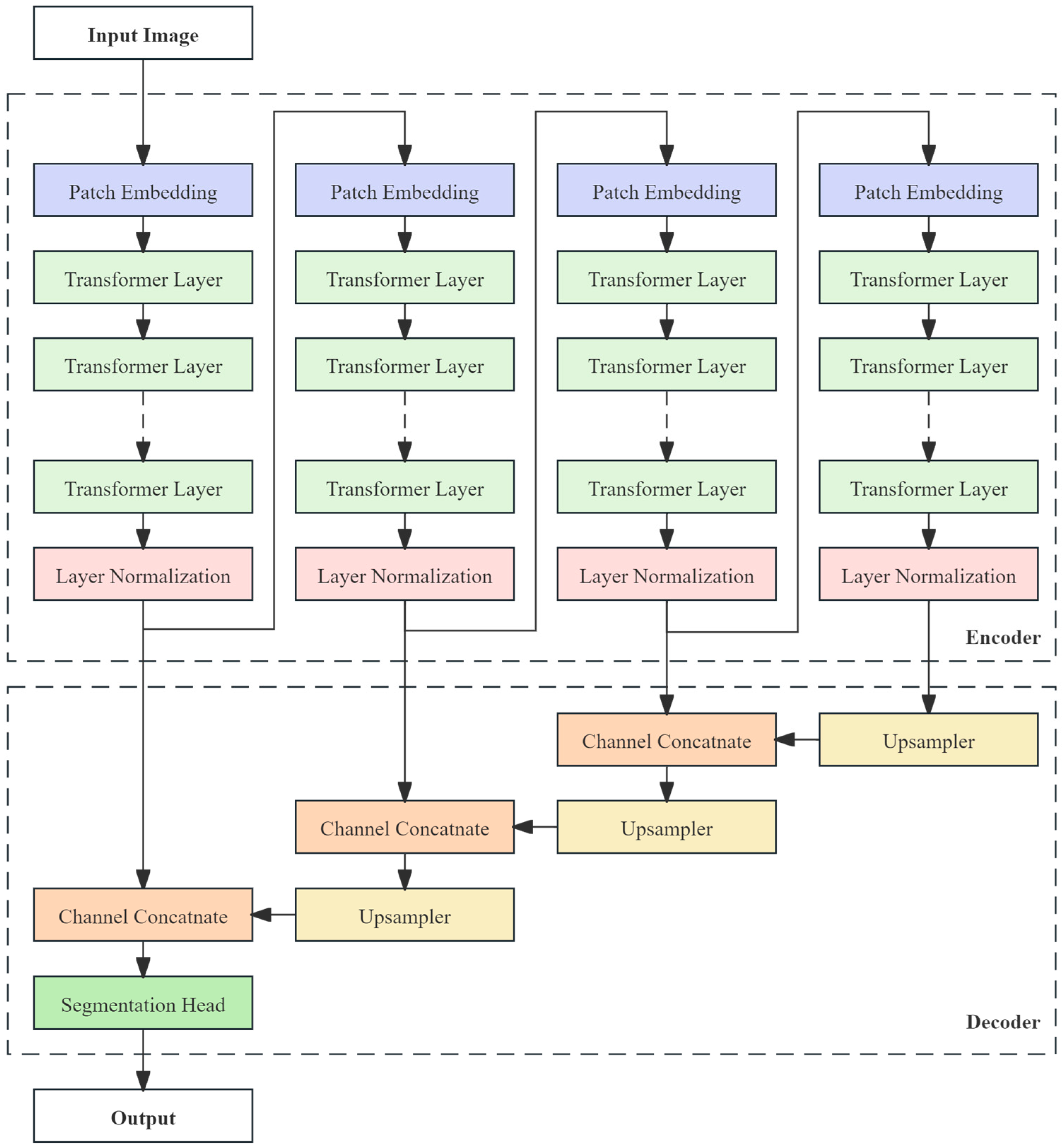
In order to realize pixel-level trace extraction, this paper proposes a multiscale Transformer trace extraction network, hereinafter referred to as IonNet, whose overall structure is shown in Figure 1. The model contains two parts, an encoder and a decoder, where the encoder consists of cascaded Transformer layers for extracting multiscale depth features from the input image, while the decoder consists of cascaded up-samplers and semantic segmentation headers, which are able to reorganize the multiscale depth features into pixel-level semantic segmentation outputs to realize trace extraction.
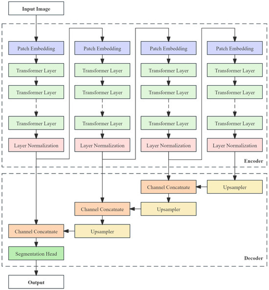
Figure 1.
Multiscale Transformer trace extraction network (IonNet) structure.
3.1. Multiscale Transformer Encoder
The single-channel rasterized ionograms input is denoted by , where and denote the height and width of the input image, respectively. The encoder converts into four depth features, , , , and , at different spatial scales, where denotes the number of channels, and the formula is expressed as follows:
where is the mapping function of the encoder.
The above multiscale encoder can be viewed as a cascade of 4 sub-encoders with a similar structure, each of which consists of structures such as a Patch Embedding Layer, Transformer Layer, Layer Normalization Layer, etc., thus realizing the extraction of deep features. The Patch Embedding Layer, while extracting deep semantic feature information, also performs spatial down-sampling on the feature data, effectively reducing the computational load for subsequent network layers. Its cascading structure enables the encoder to extract semantic information from four progressively deeper scales. This capability allows the model to understand and process image data at various abstraction levels, which is essential for enhancing the precision of trace extraction.
The above process can be expressed by the following equation:
where , , , and are the mapping functions of the four sub-encoders, respectively.
- (1)
- Patch Embedding Layer
The role of the Patch Embedding Layer is to split the input image or features into small patches and embed them so that the model can capture local features, which is very important for understanding the details in the image. In practice, Patch Embedding Layers are spatially categorized as non-overlapping or overlapping, and, in this paper, we use overlapping Patch Embedding. Although this approach consumes significantly more memory, it is very helpful for the model to understand the contextual relationships between pixels and thus improve the accuracy of segmentation.
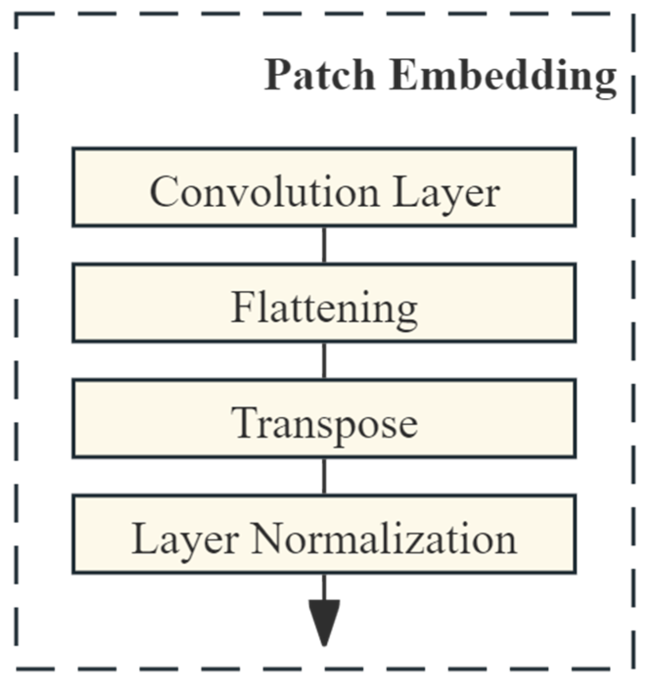
Figure 2 is the schematic diagram of the Patch Embedding Layer used in this paper. Taking the first scale as an example, the processing of the Patch Embedding Layer can be expressed as the following equation:
where denotes the mapping function of the convolutional layer, which is used to extract deep features from the input data, and spatial down-sampling can be achieved by setting the step size to more than 1. Subsequently, and denote the flattening and transposition operations on the feature data, respectively, which are used to adjust the shapes of the deep features for the convenience of the subsequent operations. Finally, corresponds to layer normalization, which is used to accelerate the training process and improve the model’s generalization ability. After the Patch Embedding Layer, the input feature is transformed into , where represents the step size of the convolutional layer, which realizes the spatial down-sampling and the extraction of deeper semantic information.
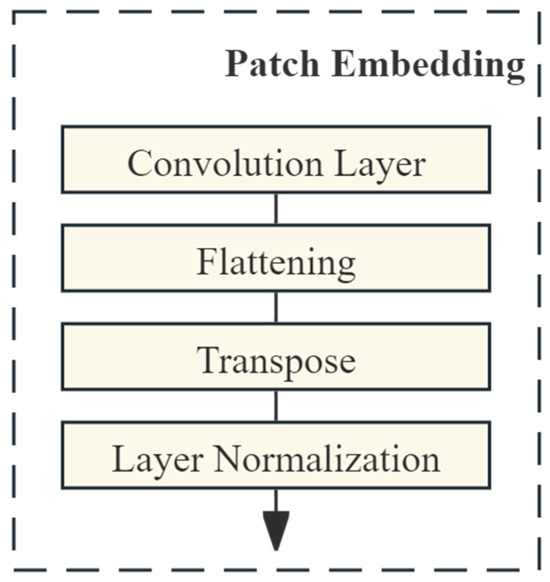
Figure 2.
Schematic diagram of Patch Embedding Layer structure.
- (2)
- Transformer Layer
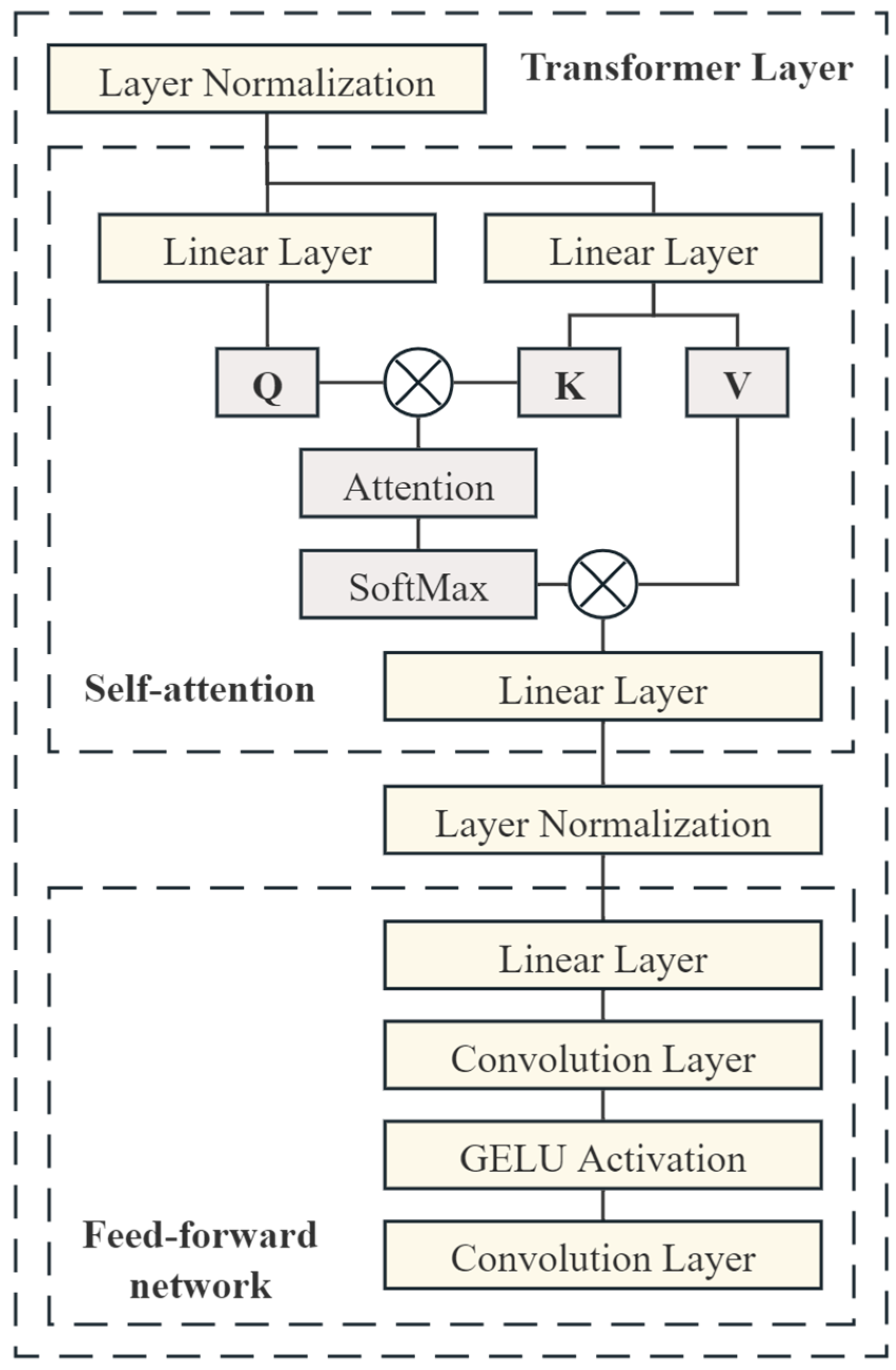
The Transformer Layer is the core of the Transformer-based network model, which usually contains two main modules: the self-attention module and feed-forward module. The principle of the self-attention module is to generate query, key, and value vectors from the input and calculate the dot product between the query and the key to obtain the attention weight distribution, which is multiplied with the value vectors and summed to obtain the weighted output. The feed-forward module generally consists of a fully connected layer and a nonlinear activation function, which nonlinearly transforms the output of the self-attention module to increase the expressive power of the model.
Specifically for the Transformer Layer used in this paper, its structure is shown in Figure 3, and its mapping function can be expressed as follows:
where and are the mapping functions of the self-attention and feed-forward modules, respectively. Assuming that is the input to the self-attention module, is first mapped to query (), key (), and value (), and the process is expressed by the following equation:
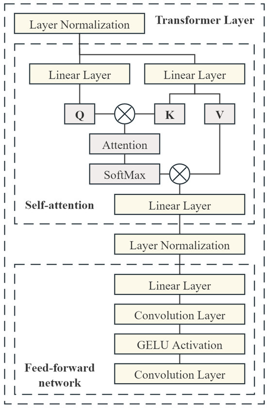
Figure 3.
Schematic diagram of Transformer Layer structure.
Subsequently, query and key compute the self-attention matrix by matrix multiplication and then the self-attention matrix will be used to weight the value, which is represented by the following equation:
where is the SoftMax activation function.
3.2. Multiscale Decoder
The multiscale decoder takes the depth feature output from the multiscale Transformer encoder as its input and increases the spatial dimensionality of these depth features. It then step-by-step increases the spatial dimensionality of the depth features using a cascading up-sampler. Ultimately, it maps the depth features into a pixel-level, semantically segmented output that matches the original image’s dimensions through a semantically segmented header. The process can be expressed by the following formula:
where , , and are the mapping functions corresponding to three up-samplers; , , and are the output features of these three up-samplers; and is the mapping function of the semantic segmentation header, whose output is the output of the whole network.
- (1)
- Up-sampler
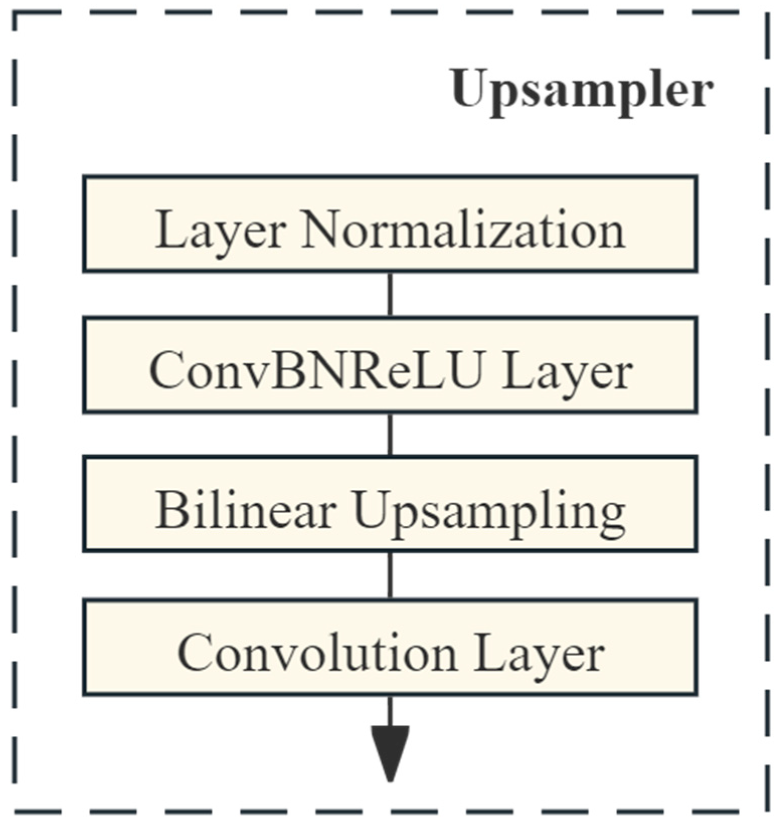
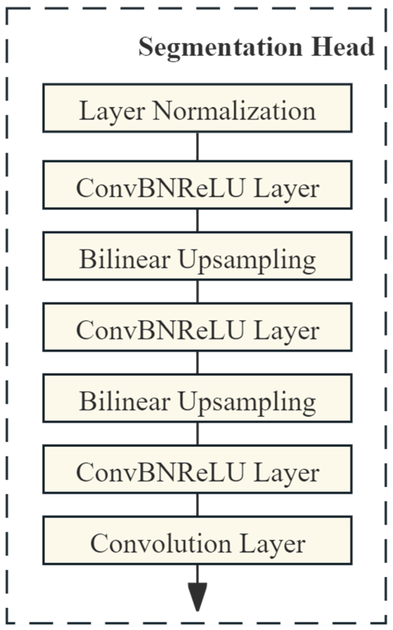
The role of the up-sampler is to boost the spatial size of the depth features by mapping from a deeper-scale feature space back to a feature space of the same scale as the input image. Usually, the up-sampler contains two main parts, as follows: the up-sampling layer, which realizes the spatial size enhancement, and the network layer, which reduces the feature size. The up-sampler used in this paper consists of layer normalization, ConvBNReLU layer (convolutional layer cascaded with batch normalization and ReLU activation function), bilinear up-sampling, and convolutional layer cascaded as shown in Figure 4, and its mapping function can be expressed as follows:
where is the mapping function for bilinear up-sampling without trainable parameters and the actual up-sampling multiplier used is 2, and is the mapping function for the ConvBNReLU layer.
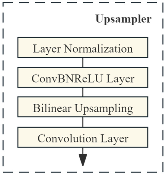
Figure 4.
Schematic diagram of up-sampler structure.
- (2)
- Semantic segmentation head
The role of the semantic segmentation header is to map the depth features to the semantic segmentation output, and each channel of the output corresponds to the segmentation result of each classification, respectively. Since the scale of the depth features input into the semantic segmentation is still smaller than the original map scale, the semantic segmentation head structure sampled in this paper has similarities with the up-sampler structure, which also consists of a cascade of network layers composed of layer normalization, ConvBNReLU layers, bilinear up-sampling, convolutional layers, etc., as shown in Figure 5, and its mapping function can be expressed as follows:
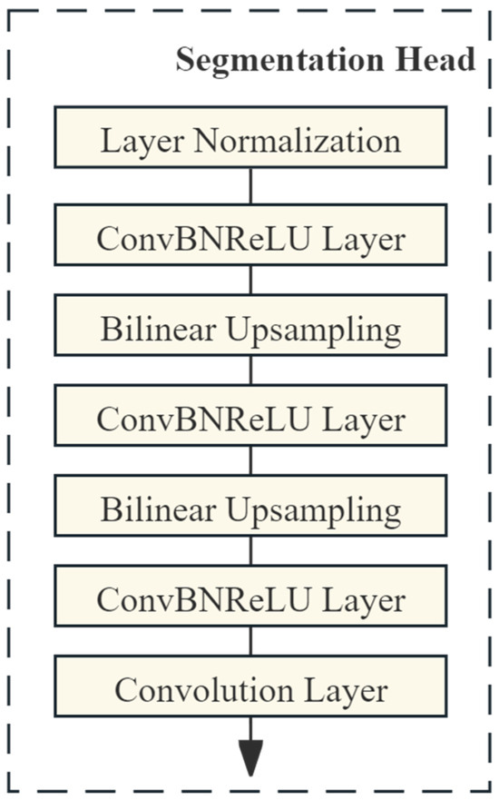
Figure 5.
Schematic diagram of segmentation head.
3.3. Loss Function
- (1)
- Cross-Entropy Loss Function
The cross-entropy loss function is often used in machine learning to measure the difference between the model’s predicted probability distribution and the probability distribution of the true labels. It is mainly used in binary or multi-classification problems to calculate the deviation between the output of a neural network and the true value, which is used to train a classification model. The cross-entropy loss function is based on the concept of entropy in information theory. Entropy is a measure of uncertainty that can be used in classification problems to measure the difference between the predicted probability distribution and the actual distribution. When the predicted probability is exactly the same as the actual distribution, the cross-entropy loss is minimized (ideally 0), indicating that the model’s prediction is very accurate; however, when the predicted probability is different from the actual distribution, the loss value increases, indicating that the model’s prediction is inaccurate. For the multi-classification problem, the formula for the cross-entropy loss function can be expressed as follows:
where is the one-hot encoding, denotes the label of the category, and is the probability distribution of the model’s prediction, indicating the probability of predicting the category.
- (2)
- OhemCrossEntropy loss function
OHEM (Online Hard Example Mining) is an online hard sample mining technique used to deal with category imbalances in target detection class tasks. The core idea of OHEM is to select those hard samples with high loss values for training in each iteration, thus making the model pay more attention to these hard-to-classify samples and improving the overall performance of the model.
OhemCrossEntropy (OHEM cross-entropy loss) is a loss function that incorporates the OHEM strategy. In the traditional cross-entropy loss function, the losses of all samples are calculated and used for gradient updating. In contrast, in the OhemCrossEntropy loss function, only the losses of those selected difficult samples (i.e., samples with loss values above a certain threshold) are used for gradient updating. In this way, the model pays more attention to those samples that are difficult to classify correctly during the training process than those that are easy to classify.
Since the proportion of the foreground pixels (E layer and F layer O wave and X wave) in the trace extraction is much smaller than that of the background pixels, and there is a significant imbalance in the proportions between the three categories of the foreground, the impact of the category imbalance problem on the performance of the network cannot be ignored. For this reason, this paper chooses to use the OhemCrossEntropy loss function to train the proposed IonNet.
4. Experiments and Analysis
4.1. System Description
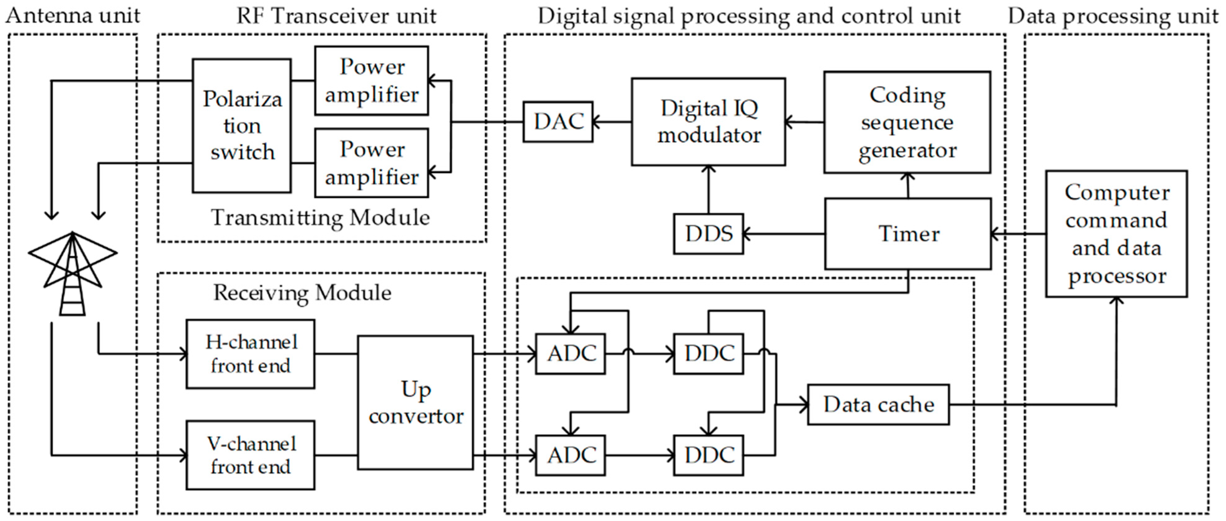
The ionospheric data come from the vertical ionosonde developed by Key Laboratory of Microwave Remote Sensing Technology, National Space Science Center, Chinese Academy of Sciences. The vertical ionosonde, situated in Yinchuan City, Ningxia Hui Autonomous Region, China, monitors ionosphere variations over western China. In addition, the ionosonde is composed of an antenna unit, an RF transceiver unit, a digital signal processing and control unit, and a data processing unit. A system block diagram is shown below [28,29].
The vertical ionosonde uses high-frequency pulses as the transmitting signals, and carriers with different frequencies are transmitted to the ionosphere. Reflections occur when the emitted frequency is equal to that of the ionospheric plasma frequency, and the ionograms can be obtained directly by measuring the time when the echo reaches the receiver. The system specifications are listed in Table 1. The block diagram of the vertical ionosonde system is shown in Figure 6.

Table 1.
CCDI system specifications.
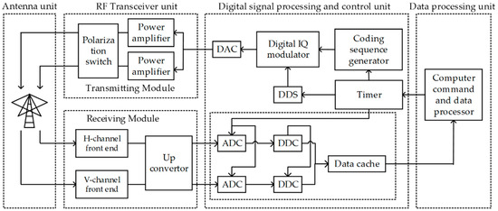
Figure 6.
Block diagram of the Yinchuan vertical ionosonde.
The detection frequency range of the ionosonde is 1.2–30 MHz, and the calculated virtual height is between 67.5 km and 560.1 km. There are three types of time data acquisition methods, and the different frequency steps correspond to different acquisition times, as follows: 25 kHz, 50 kHz, and 100 kHz correspond to 7.36 min, 3.68 min, and 1.84 min, respectively. Due to the system setting, the frequency step of the transmitting signal of the Yinchuan vertical ionosonde is always 25 kHz. The ionograms used in this paper also have a frequency interval of 25 kHz, which has a higher frequency resolution.
4.2. Dataset
A dataset was established for model training and testing based on the real echo data collected with the Yinchuan vertical ionosonde. Currently, the ionosonde system is set to collect the full ionospheric echo information with the frequency range of 1.2~12.9 MHz (horizontal coordinate) and the height range of 67.5~560.1 km (vertical coordinate), where the intensity unit of the echo signals is Volt. These raw signals are not directly input to the neural network for processing. In addition, in order to provide credentials for use in neural network training and evaluation, the truth values of the segmentation results need to be labeled. Therefore, two preprocessing steps are performed on the data: discretization and data labeling.
Since the echo data collected with the vertical ionosonde are located in continuous “frequency–height” coordinates, and the neural network can only handle discrete data, it is necessary to map the original data to discrete frequency–height coordinates. In order to take into account the resolution of the ionograms and the processing capability of the neural network, the original frequency–height data are mapped into a rasterized frequency–height map with 50 kHz as the minimum frequency interval and 3km as the minimum altitude interval, and the original signal strengths that fall into the same raster are summed up. Eventually, the frequency–height data from one measurement are mapped into a rasterized 256 × 160 ionogram, corresponding to a frequency range of 0~12.8 MHz and a height range of 24~504 km.
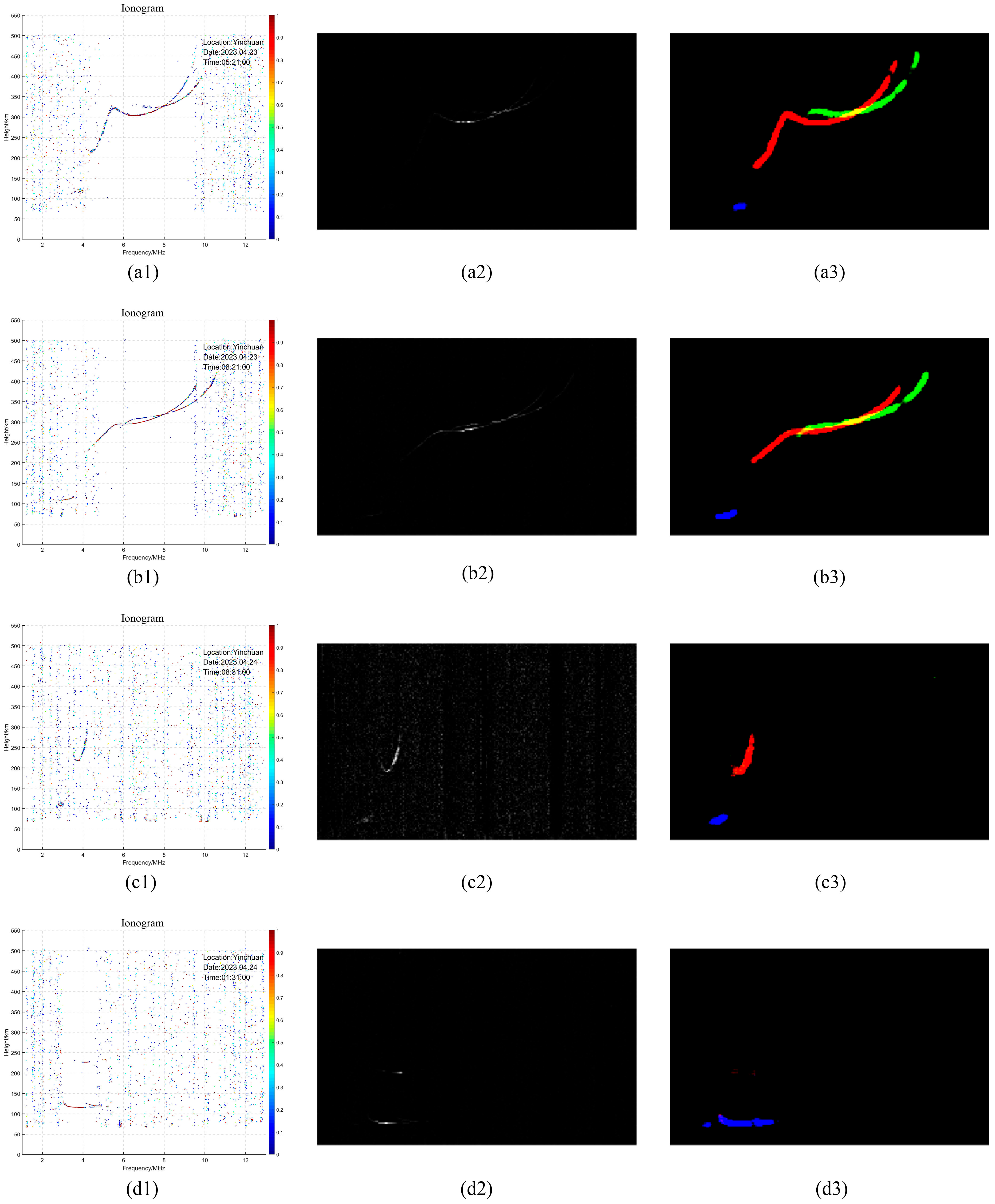
In order to obtain the true value of the trace extraction, this paper labels the positions of the E layer and O and X waves in the F layer of the rasterized ionograms (the annotation tool: Labelme, https://github.com/labelmeai/labelme#anaconda, accessed on 26 March 2023). A total of 2523 sets of data were collected and labeled during the experiment, of which 2518 sets were used as the training data and 505 sets as the test data. The ionograms, corresponding gray-scale plots, and truth plots are shown below in Figure 7.
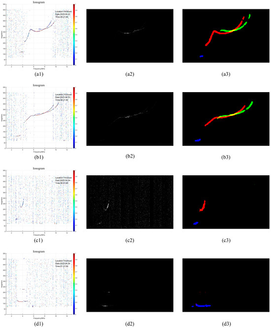
Figure 7.
Ionograms, rasterized ionograms, and labels. (a1–d1) shows the original ionograms. (a2–d2,a3–d3) are the corresponding gray scale images and ground truth images respectively. (a3–d3), the E layer is shown as the blue part, the F layer O-wave is the red part, and the X-wave is the green part.
4.3. Experiment Setup
4.3.1. State-of-the-Art Methods
In order to provide a comprehensive evaluation of the performance of the proposed multiscale Transformer network and to explore its practical value in trace extraction applications, this chapter compares the proposed network with a series of state-of-the-art semantic segmentation network architectures. The network models compared include the following:
- (1)
- FCN (Fully Convolutional Network): FCN is a pioneering work in the field of semantic segmentation that replaces the fully connected layer with a convolutional layer, enabling the network to accept input images of arbitrary size and output segmentation maps of corresponding size [7].
- (2)
- U-Net: U-Net is a popular network for medical image segmentation with a symmetric U-shaped structure that combines deep features with shallow features through jump connections to preserve edge information [9].
- (3)
- CCNet (Criss-Cross Network): CCNet captures long-distance dependencies between features by means of the Recurrent Criss-Cross Attention Module (RCCA), which helps to provide denser contextual information and thus aids in image understanding [10].
- (4)
- DeepLabV3+: DeepLabV3+ uses Atrous Convolution and Spatial Pyramid Pooling (ASPP) modules in its encoder to introduce multiscale information. In addition, it introduces a decoder module to improve the accuracy of the segmentation boundaries by fusing the underlying and higher-level features [30].
- (5)
- EncNet (Context Encoding Network): EncNet introduces the Context Encoding Module (CEM) on top of the pre-trained ResNet to strengthen the network by utilizing the null convolution to better utilize the global context information [31].
- (6)
- OCRNet (Occlusion Reasoning Network): OCRNet deals with the occlusion problem in the scene by introducing an occlusion inference mechanism, which improves the accuracy of segmentation by learning the relationship between the occluded and non-occluded regions [32].
- (7)
- PSPNet (Pyramid Scene Parsing Network): PSPNet uses Pyramid Scene Parsing Pooling (PSPNet) to capture contextual information at different scales, which helps the model to understand the scene at different scales [33].
- (8)
- SETR (Segmentation Transformer): SETR applies the Transformer architecture to semantic segmentation, capturing global dependencies through a self-attention mechanism while using an encoder–decoder structure to process image sequences [34].
4.3.2. Implementation Details
In the training phase of this paper, a series of strategies are used to enhance the performance and generalization ability of the model. The input image is cropped into blocks of fixed-size pixels, and random horizontal flip and rotation operations are introduced for data enhancement. These transformations not only increase the diversity of the training samples, but also simulate the different positions and shapes of the traces that may appear in the rasterized ionograms, which improves the model’s adaptability in the face of unknown data.
For the selection of optimization algorithms, the AdamW optimizer, as well as the polynomial learning rate decay strategy, were used to stabilize the training process by dynamically adjusting the learning rate. The learning rate is initialized and gradually decays to a final value of 0 through a polynomial decay strategy. The selection of these parameters is based on extensive experiments and literature research to ensure that the model is able to maintain fast convergence while avoiding falling into local minima. As for the parameter settings of the comparison methods, this paper tries to follow the configurations in the methods’ respective original paper as much as possible to ensure that each model can be compared at the optimal state of its design, making the experimental results more convincing.
In order to ensure the fairness and comparability of the experimental results, the training batch size of all of the methods is set to eight, and the number of iterations (epoch) is about 20,000. Such a setting aims to give each model enough training time to fully learn the patterns in the data. In addition, all models are implemented based on the Paddle-Paddle deep learning framework and trained on an NVIDIA GTX3060 GPU with 12 GB of graphics memory.
In the evaluation phase, the test images, on the other hand, are not subjected to any data enhancement, such as cropping, rotating, or inverting, and are inputted into the trained models to be evaluated with a batch size of one in order to objectively evaluate the performance of the network.
4.3.3. Evaluation Indicators
In order to objectively evaluate the performance of the proposed multiscale Transformer network and a series of comparison methods, this paper uses a series of evaluation metrics commonly used in semantic segmentation, including the following:
- (1)
- mIoU (mean intersection union): mIoU calculates the IoU (intersection and concurrency ratio) of each category and then takes the average of these IoUs as a comprehensive index, which can reflect the segmentation effect of the model on different categories. The result ranges from 0 to 1, and the closer it is to 1, the higher the accuracy rate. Its specific calculation formula is as follows:where TP denotes True Positive, TN denotes True Negative, FP denotes False Positive, and FN denotes False Negative, denoting different categories.
- (2)
- Kappa coefficient (Cohen’s Kappa): The principle of Kappa coefficient is to measure the degree of consistency between two evaluators (or evaluation methods) in categorizing the same dataset, not only considering the actual consistency (i.e., the proportion of the two evaluators who give the same classification), but also considering the random consistency (i.e., the proportion of consistency that would be expected in a random situation), taking the range of values from −1 (complete inconsistency) to 1 (complete consistency), with 0 indicating random consistency. The process of calculating the Kappa coefficient can be expressed as follows:where and denote the observed consistency proportion and the desired consistency proportion, respectively.
- (3)
- Dice coefficient: The Dice coefficient serves as a valuable statistical metric for quantifying the degree of similarity between two sets, particularly in the context of evaluating the alignment between a model’s segmentation predictions and the actual annotations. It is calculated by taking the ratio of the 2-fold sum of the intersection (overlap) between the binary images—representing the model’s segmentation (foreground and background)—and the true binary labeled images. This coefficient provides a measure that encapsulates both the accuracy and the completeness of the segmentation, with the computational formula given by the following:
The value of the Dice coefficient ranges from 0 to 1, with 1 indicating perfect consistency and 0 indicating no consistency.
- (4)
- AUC-ROC (area under the receiver operating characteristic curve): AUC-ROC is defined as the area under the ROC curve, which provides a single metric to assess the overall performance of the classifier. The value of AUC ranges from 0 to 1, where 1 indicates a perfect classifier (i.e., that correctly distinguishes between positive and negative samples in all cases), 0.5 indicates a random guess, and less than 0.5 indicates a classifier that does not perform as well as a random guess. The AUC-ROC formulation does not directly involve the semantic segmentation of images, but rather calculates the area under the ROC curve by the following steps: (i) calculating the TPR and the FPR for different thresholds; (ii) in the ROC space (FPR vs. TPR); (iii) plotting a point for each threshold (FPR, TPR); and (iv) calculating the area under the curve formed by these points, which is the AUC value.
In addition, the performance of a neural network is generally positively correlated with its size and computation, and a neural network with a smaller size and computation has a more reasonable structure for the same semantic segmentation performance. Therefore, this paper also evaluates the size and computation of all models using the indicators of trainable parameter count and floating-point operations, respectively.
4.4. Experimental Results
4.4.1. Comparison of Trace Extraction Performance
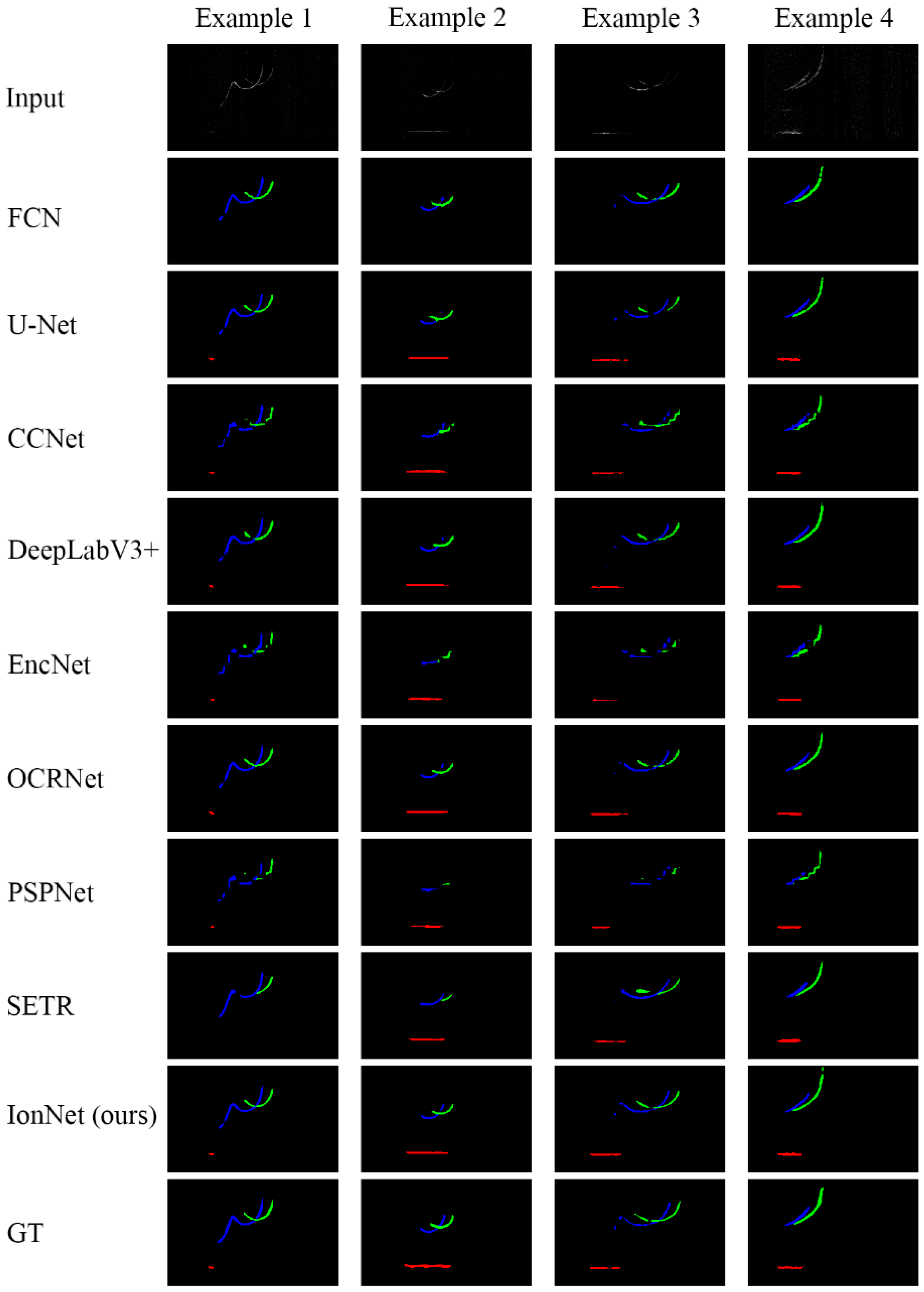
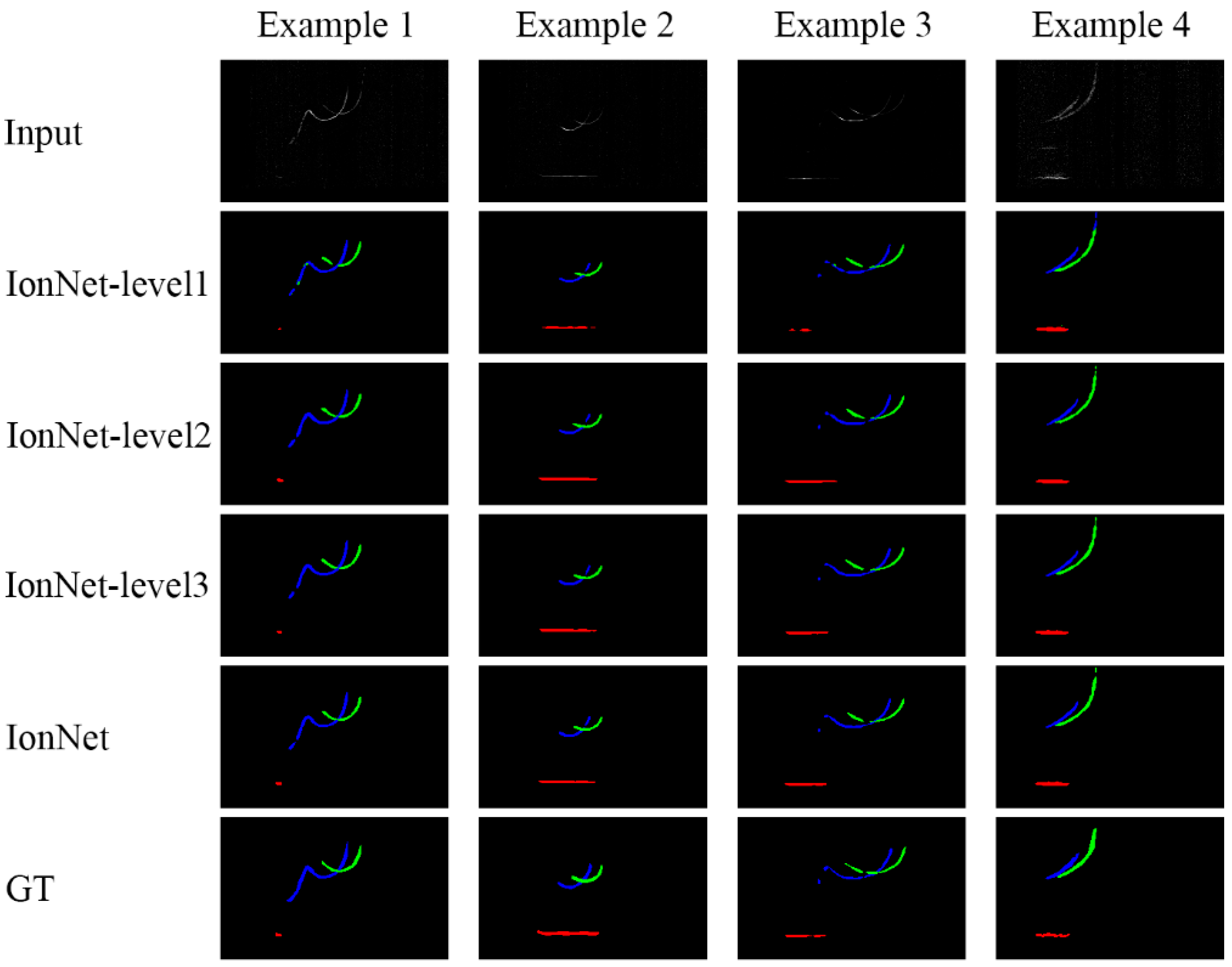
For quantitative evaluation, the evaluation results of all methods on the evaluation dataset are shown in Table 2, where the boldface represents the optimal result, and the underline represents the sub-optimal result. An example of reconstruction results on a partial evaluation dataset is shown in Figure 8.

Table 2.
Quantitative experimental results of trace extraction.

Figure 8.
Examples of trace extraction results of different models. Red represents E layer, blue represents F layer O wave, and green represents F layer X wave.
From the above experimental results, it can be seen that the IonNet trace extraction network proposed in this paper shows the best performance on all of the semantic segmentation effect evaluation metrics, mIoU, Kappa, Dice, and AUC-ROC, as well as the best visual perception of trace extraction, which indicates that IonNet has a significant advantage in terms of trace extraction accuracy and consistency. Meanwhile, IonNet has the best computation amount and the second-best number of trainable parameters among all of the methods, which further confirms its high computational efficiency while maintaining high performance, which is especially important for resource-constrained application scenarios. In contrast, DeepLabV3+ and OCRNet also perform relatively well, achieving superior trace extraction accuracy with a relatively moderate number of parameters and computational effort. In addition, the U-Net model also performs well in the performance metrics, which, as a network model proposed in 2015, is a good indication of the rationality of its structural design. Overall, the IonNet model demonstrated the best performance and efficiency in this study, proving the effectiveness and superiority of its structure.
In addition, the above evaluation results are averaged over all of the categories of trace extraction, while the categories involved in trace extraction are background, E-layer, X-layer, and O-layer. There is a significant difference in the pixel percentage of each category, in which the background has the highest pixel percentage, and the accurate segmentation of the background will result in a higher overall segmentation accuracy. However, this does not necessarily mean that the model is also more accurate for the more concerned E, X, and O layers. This reflects the common problem of sample size imbalance in image semantic segmentation. Therefore, this paper also evaluates the semantic segmentation results of the network by category, as shown in Table 3.

Table 3.
Quantitative experimental results of trace extraction by category.
From the above table, it can be seen that the IonNet model proposed in this paper exhibits the highest mIoU scores in all categories, and the accuracy of the three categories of E layer and O/X waves in the F2 layer is relatively similar, which suggests that IonNet not only has a significant advantage in the overall trace extraction performance, but also better copes with the problem of the imbalance of sample categories. In contrast, U-Net, DeepLabV3+, and OCRNet also performed relatively well. It is worth noting that the FCN model, while having better mIoU for the background, O, and X traces, is very ineffective in segmenting the E layer, which has the smallest percentage of the number of samples, suggesting that the network does not have a targeted design for the sample imbalance problem.
4.4.2. Ablation Analysis
In order to further assess the rationality and effectiveness of the structural design of the multiscale Transformer trace extraction network proposed in this paper, a series of ablation experiments were specifically designed. In these experiments, certain key components in the network were removed or specific parameter settings were adjusted in a targeted manner as a way to observe the specific effects of these changes on the network performance. By comparing the results before and after the experiments, a clearer understanding of the role of each structural element in the trace extraction process and how they interact to improve the overall network performance can be achieved. This analysis not only helps to optimize the network structure, but also provides a valuable reference for future related research.
In this section of the study, an ablation analysis of the network structure for multiscale feature encoding and decoding is performed to assess its design soundness. In order to achieve this goal, several network variants with different scales are constructed, and their trace extraction capabilities are comparatively investigated. The statistics of the evaluation metrics are shown in Table 4; moreover, to compare the network performance more intuitively, examples of the trace extraction results of the different network variants are shown in Figure 9. From these results, it can be seen that the overall performance of the model shows a decreasing trend when the scales of feature encoding and decoding are reduced. The more scales that are reduced, the more significant the decrease in model performance becomes. This not only illustrates the importance of feature encoding and decoding scales in the trace extraction task, but also the necessity of rationally configuring the scales when designing the network structure.

Table 4.
Quantitative experimental results of trace extraction of different variants of IonNet.
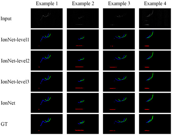
Figure 9.
Examples of trace extraction results of IonNet with different scales. Red represents E layer, blue represents F layer O wave, and green represents F layer X wave.
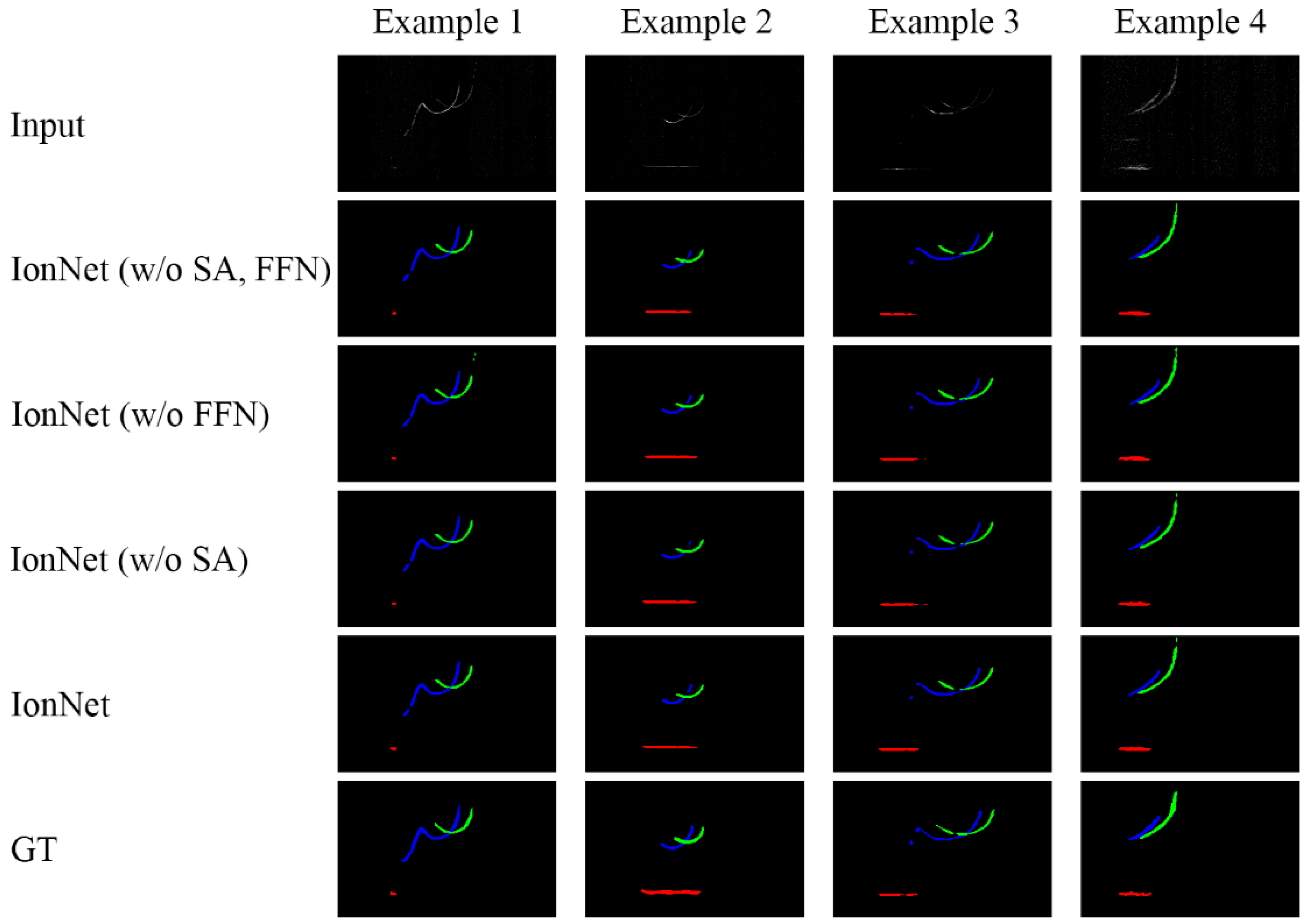
In this section of the study, an ablation analysis of the Transformer structure is also performed to assess its design soundness. To achieve this goal, several variants of the Transformer were constructed by replacing the self-attention module and the feed-forward network module of the original Transformer with ordinary convolutional layers, respectively. The statistics of the evaluation metrics are shown in Table 5 and the results of the trace extraction for the different network variants are shown below. From these results, it can be seen that the performance of the IonNet composed of the new Transformer variant shows a significant degradation, whether the self-attention module or the feed-forward network module is removed. Not only do these two modules each play an important role, but effective collaboration between them is crucial for model performance improvement. This proves the rationality of the structural design of the self-attention module and the feedforward network module in this paper, as well as the effective collaboration between the attention module and the feed-forward network module and the structural design of the Transformer module. The result is shown in Figure 10.

Table 5.
Quantitative experimental results of trace extraction of IonNet with different variants of Transformer.
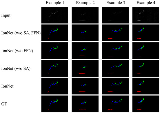
Figure 10.
Examples of trace extraction results of IonNet with different Transformer variants. Red represents E layer, blue represents F layer O wave, and green represents F layer X wave.
Based on the above evaluation, labeling, and analysis, the Transformer network has a high retention of echo integrity when extracting the echo traces of each layer in the ionograms, especially the E layer, which has a positive effect on the subsequent inversion, and the accuracy of the inversion results is improved.
5. Discussion and Conclusions
In order to extract traces from the ionograms for subsequent electron density inversion, we propose a trace extraction method based on a multiscale Transformer network. Trace extraction, i.e., segmenting the regions belonging to the E- and F2-layer O- and X-waves from the ionograms, is very similar to the goal of semantic segmentation tasks in computer vision; therefore, this paper transforms trace extraction into the semantic segmentation task in computer vision and realizes it by using a deep neural network method. Firstly, real frequency–height data are collected using a vertical ionosonde, and the dataset is obtained by preprocessing means such as discretization and labeling, and then the neural network is trained with the dataset. Then, a multiscale Transformer network is designed, which is able to encode and decode semantic information from multiple feature scales and realize accurate pixel-level semantic segmentation. Finally, the proposed network is compared with a series of state-of-the-art semantic segmentation networks, and ablation analysis is performed. Experiments demonstrate the effectiveness of the structural design of the proposed network and prove the feasibility of using neural networks for the trace extraction task.
The application of the multiscale Transformer model to the extraction of ionogram echo traces is an innovative attempt. In this application, the capabilities of the multiscale Transformer model are newly extended, leaping from processing text sequences to processing image data, especially those ionograms with high complexity and dynamic changes. These images usually contain rich spatial and frequency information, reflecting the vertical distribution of ionospheric electron density.
In the task of echo trace extraction from ionospheric ionograms, the multiscale Transformer model needs to deal with not only the sequence data, but also the spatial dimension of the images. This challenge has motivated researchers to improve and optimize the multiscale Transformer model to better accommodate the characteristics of the image data.
In addition, the parallel computing capability of the multiscale Transformer model shows significant advantages when dealing with large-scale ionospheric data. Compared to traditional convolutional neural networks (CNN), the multiscale Transformer model is able to utilize computational resources more efficiently when processing large-scale data, accelerating the training and inference processes. However, only E layer and F2 layer O/X waves were considered in the construction of the dataset in this paper, and more case data were not labeled. The scale of the dataset and the types of spatial activities covered also need to be expanded. These improvements to the dataset may further enhance the robustness and generalization ability of the neural network.
In conclusion, the application of the multiscale Transformer neural network to the extraction of echo traces of ionospheric ionograms not only broadens the application field of the multiscale Transformer model, but also provides new perspectives and methods for ionospheric research and plays a certain role in the development of subsequent autonomous inversion software. With the continuous progress of deep learning technology, it is reasonable to believe that the multiscale Transformer model will play an increasingly important role in ionospheric research and other related fields.
Author Contributions
Conceptualization, S.H.; methodology, S.H.; validation, S.H.; formal analysis, S.H.; investigation, S.H.; resources, W.G.; data curation, C.W.; writing—original draft preparation, S.H.; writing—review and editing, S.H. and C.W.; supervision, W.G.; project administration, W.G.; funding acquisition, W.G. and C.W. All authors have read and agreed to the published version of the manuscript.
Funding
This research is based on the National space infrastructure common application support platform and supported by National Development and Reform Commission, and the funding numbers are E0A203020F and E0A203010F. This research was also supported by the Natural Science Foundation of Hainan Province, China, and the funding number is 423MS11.
Data Availability Statement
The original contributions presented in the study are included in the article, further inquiries can be directed to the corresponding author.
Acknowledgments
Thanks to all those who contributed to the articles.
Conflicts of Interest
The authors declare no conflicts of interest.
References
- John, M. Goodman the Ionosphere. In Space Weather & Telecommunications; Kluwer Academic Publishers: Boston, MA, USA, 2005; pp. 81–173. [Google Scholar]
- Davies, K. Ionospheric Radio; P. Peregrinus on behalf of the Institution of Electrical Engineers: London, UK, 1989; ISBN 086341186X. [Google Scholar]
- Reinisch, B.W.; Xueqin, H. Automatic Calculation of Electron Density Profiles from Digital Ionograms: 1. Automatic O and X Trace Identification for Topside Ionograms. Radio Sci. 1982, 17, 421–434. [Google Scholar] [CrossRef]
- Reinisch, B.W.; Xueqin, H. Automatic Calculation of Electron Density Profiles from Digital Ionograms: 3. Processing of Bottomside Ionograms. Radio Sci. 1983, 18, 477–492. [Google Scholar] [CrossRef]
- Xueqin, H.; Reinisch, B.W. Automatic Calculation of Electron Density Profiles from Digital Ionograms: 2. True Height Inversion of Topside Ionograms with the Profile-fitting Method. Radio Sci. 1982, 17, 837–844. [Google Scholar] [CrossRef]
- Bilitza, D.; Pezzopane, M.; Truhlik, V.; Altadill, D.; Reinisch, B.W.; Pignalberi, A. The International Reference Ionosphere Model: A Review and Description of an Ionospheric Benchmark. Rev. Geophys. 2022, 60, e2022RG000792. [Google Scholar] [CrossRef]
- Long, J.; Shelhamer, E.; Darrell, T. Fully Convolutional Networks for Semantic Segmentation. In Proceedings of the 2015 IEEE Conference on Computer Vision and Pattern Recognition (CVPR), Boston, MA, USA, 7–12 June 2015; pp. 3431–3440. [Google Scholar]
- Chen, L.C.; Papandreou, G.; Kokkinos, I.; Murphy, K.; Yuille, A.L. Yuille DeepLab: Semantic Image Segmentation with Deep Convolutional Nets, Atrous Convolution, and Fully Connected CRFs. IEEE Trans. Pattern Anal. Mach. Intell. 2017, 40, 834–848. [Google Scholar] [CrossRef] [PubMed]
- Ronneberger, O.; Fischer, P.; Brox, T. U-Net: Convolutional Networks for Biomedical Image Segmentation. In Medical Image Computing and Computer-Assisted Intervention—MICCAI 2015: 18th International Conference, Munich, Germany, 5–9 October 2015; Springer: Cham, Switzerland, 2015. [Google Scholar]
- Huang, Z.; Wang, X.; Wei, Y.; Huang, L.; Shi, H.; Liu, W.; Huang, T.S. CCNet: Criss-Cross Attention for Semantic Segmentation. In Proceedings of the IEEE/CVF International Conference on Computer Vision, Seoul, Republic of Korea, 27 October–2 November 2019. [Google Scholar]
- Lu, H. Study on Automatic Scaling of E, Es in Ionogram Based on Image Processing; Ocean University of China: Qingdao, China, 2013. [Google Scholar]
- Xu, G. Study on Parameters Extraction in Ionogram Based on Image Processing; Ocara University of China: Qingdao, China, 2014. [Google Scholar]
- Guo, W.; Sun, X.; Ji, Y.; Jia, X. Ionospheric TEC Prediction Based on QPSO-LSTM Model. Chin. J. Space Sci. 2024. [Google Scholar]
- Ding, Z. Studies on Autoscaling and Analysis of Ionograms; Wuhan Institute of Physics and Mathematics & Institute of Geology and Geophysics, Chinese Academy of Sciences: Wuhan, China, 2006. [Google Scholar]
- Jiang, C.; Yang, G.; Zhao, Z.; Zhang, Y.; Zhu, P.; Sun, H.; Zhou, C. A Method for the Automatic Calculation of Electron Density Profiles from Vertical Incidence Ionograms. J. Atmos. Sol.-Terr. Phys. 2014, 107, 20–29. [Google Scholar] [CrossRef]
- Jiang, C.; Liu, Z.; Zhao, C.; Liu, T.; Yang, G.; Shen, H.; Huang, W. A Regional Model of Topside Ionospheric Effective Scale Heights Derived from Ionosonde and GNSS TEC. Space Weather 2023, 21, e2023SW003515. [Google Scholar] [CrossRef]
- Wu, R. Automatic Scaling of F Layer for Ionogram Based on BP Neural Network; South-Central University for Nationalities: Wuhan, China, 2015. [Google Scholar]
- Mochalov, V.; Mochalova, A. Application of Deep Learning to Recognize Ionograms. In Proceedings of the 2019 Russian Open Conference on Radio Wave Propagation (RWP), Kazan, Russia, 1–6 July 2019; pp. 477–479. [Google Scholar]
- Xiao, Z.; Wang, J.; Li, J.; Zhao, B.; Hu, L.; Liu, L. Deep-Learning for Ionogram Automatic Scaling. Adv. Space Res. 2020, 66, 942–950. [Google Scholar] [CrossRef]
- Luwanga, C.; Fang, T.; Chandran, A.; Lee, Y. Automatic Spread-F Detection Using Deep Learning. Radio Sci. 2022, 57, 1–16. [Google Scholar] [CrossRef]
- Liu, Z.; Lin, Y.; Cao, Y.; Hu, H.; Wei, Y.; Zhang, Z.; Lin, S.; Guo, B. Swin Transformer: Hierarchical Vision Transformer Using Shifted Windows. In Proceedings of the IEEE/CVF International Conference on Computer Vision, Montreal, BC, Canada, 11–17 October 2021. [Google Scholar]
- Dosovitskiy, A.; Beyer, L.; Kolesnikov, A.; Weissenborn, D.; Zhai, X.; Unterthiner, T.; Dehghani, M.; Minderer, M.; Heigold, G.; Gelly, S.; et al. An Image Is Worth 16x16 Words: Transformers for Image Recognition at Scale. arXiv 2020, arXiv:2010.11929. [Google Scholar]
- He, K.; Chen, X.; Xie, S.; Li, Y.; Dollár, P.; Girshick, R. Masked Autoencoders Are Scalable Vision Learners. In Proceedings of the IEEE/CVF Conference on Computer Vision and Pattern Recognition, New Orleans, LA, USA, 18–24 June 2022. [Google Scholar]
- Jaegle, A.; Gimeno, F.; Brock, A.; Zisserman, A.; Vinyals, O.; Carreira, J. Perceiver: General Perception with Iterative Attention. In Proceedings of the International Conference on Machine Learning, Online, 18–24 July 2021. [Google Scholar]
- Fan, H.; Xiong, B.; Mangalam, K.; Li, Y.; Yan, Z.; Malik, J.; Feichtenhofer, C. Multiscale Vision Transformers. In Proceedings of the IEEE/CVF International Conference on Computer Vision, Montreal, BC, Canada, 11–17 October 2021. [Google Scholar]
- Chen, C.-F.; Fan, Q.; Panda, R. CrossViT: Cross-Attention Multi-Scale Vision Transformer for Image Classification. In Proceedings of the IEEE/CVF International Conference on Computer Vision, Montreal, BC, Canada, 11–17 October 2021. [Google Scholar]
- Shao, K.; Wang, M.; Wang, G. Transformer-Based Multiscale Remote Sensing Semantic Segmentation Network. CAAI Trans. Intell. Syst. 2024. [Google Scholar]
- Han, S.; Guo, W.; Liu, P.; Wang, T.; Wang, C.; Fang, Q.; Yang, J.; Li, L.; Liu, D.; Huang, J. Chaotic Coding for Interference Suppression of Digital Ionosonde. Remote Sens. 2023, 15, 3747. [Google Scholar] [CrossRef]
- Jin, M.; Guo, W.; Liu, P.; Wang, C. Design of Digital Control System for High-Performance Ionosonde Based on FPGA. Chin. J. Space Sci. 2021, 41, 580–588. [Google Scholar] [CrossRef]
- Chen, L.-C.; Zhu, Y.; Papandreou, G.; Schroff, F.; Adam, H. Encoder-Decoder with Atrous Separable Convolution for Semantic Image Segmentation. In Proceedings of the European Conference on Computer Vision (ECCV), Munich, Germany, 8–14 September 2018. [Google Scholar]
- Zhang, H.; Dana, K.; Shi, J.; Zhang, Z.; Wang, X.; Tyagi, A.; Agrawal, A. Context Encoding for Semantic Segmentation. In Proceedings of the IEEE Conference on Computer Vision and Pattern Recognition, Salt Lake City, UT, USA, 18–23 June 2018. [Google Scholar]
- Yuan, Y.; Chen, X.; Chen, X.; Wang, J. Segmentation Transformer: Object-Contextual Representations for Semantic Segmentation. arXiv 2019, arXiv:1909.11065. [Google Scholar]
- Zhao, H.; Shi, J.; Qi, X.; Wang, X.; Jia, J. Pyramid Scene Parsing Network. In Proceedings of the IEEE Conference on Computer Vision and Pattern Recognition, Honolulu, HI, USA, 21–26 July 2017. [Google Scholar]
- Zheng, S.; Lu, J.; Zhao, H.; Zhu, X.; Luo, Z.; Wang, Y.; Fu, Y.; Feng, J.; Xiang, T.; Torr, P.H.S.; et al. Rethinking Semantic Segmentation from a Sequence-to-Sequence Perspective with Transformers. In Proceedings of the IEEE/CVF Conference on Computer Vision and Pattern Recognition, Nashville, TN, USA, 20–25 June 2021. [Google Scholar]
Disclaimer/Publisher’s Note: The statements, opinions and data contained in all publications are solely those of the individual author(s) and contributor(s) and not of MDPI and/or the editor(s). MDPI and/or the editor(s) disclaim responsibility for any injury to people or property resulting from any ideas, methods, instructions or products referred to in the content. |
© 2024 by the authors. Licensee MDPI, Basel, Switzerland. This article is an open access article distributed under the terms and conditions of the Creative Commons Attribution (CC BY) license (https://creativecommons.org/licenses/by/4.0/).

