Monitoring the Vertical Variations in Chlorophyll-a Concentration in Lake Chaohu Using the Geostationary Ocean Color Imager

Abstract

Due to the external environment and the buoyancy of cyanobacteria, the inhomogeneous vertical distribution of phytoplankton in eutrophic lakes affects remote sensing reflectance (R_rs) and the inversion of surface chlorophyll-a concentration (Chla). In this study, vertical profiles of Chla(z) (where z is the water depth) and field R_rs (R_rs_F) were collected and utilized to retrieve the vertical profiles of Chla in Lake Chaohu in China. Chla(z) was categorized into vertically uniform (Type 1: N = 166) and vertically non-uniform (Type 2: N = 58) types. Based on the validation of the atmospheric correction performance of the Geostationary Ocean Color Imager (GOCI), a Chla(z) inversion model was developed for Lake Chaohu from 2011 to 2020 using GOCI R_rs data (R_rs_G). (1) Five functions of non-uniform Chla(z) were compared, and the best result was found for Chla(z) = a × exp(b × z) + c (R² = 0.98, RMSE = 38.15 μg/L). (2) A decision tree of Chla(z) was established with the alternative floating algae index (AFAI_Rrs), the fluorescence line height (FLH), and wind speed (WIN), where the overall accuracy was 89% and the Kappa coefficient was 0.79. The Chla(z) inversion model for Type 1 was established using the empirical relationship between Chla (z = surface) and AFAI_Rrs (R² = 0.58, RMSE = 10.17 μg/L). For Type 2, multivariate regression models were established to estimate the structural parameters of Chla(z) combined with R_rs_G and environmental parameters (R² = 0.75, RMSE = 72.80 μg/L). (3) There are obvious spatial variations in Chla(z), especially from the water surface to a depth of 0.1 m; the largest diurnal variations were observed at 12:16 and 13:16 local time. The Chla(z) inversion method can determine Chla in different layers of each pixel, which is important for the scientific assessment of phytoplankton biomass and lake carbon and can provide vertical information for the short-term prediction of algal blooms (and the generation of corresponding warnings) in lake management.

1. Introduction

Influenced by human activities and climate change, the eutrophication of lakes has increased [1], and the water-ecological problems caused by the decline in water quality and increase in cyanobacteria blooms have become increasingly serious [2]. Chlorophyll-a (Chla) is the main pigment in phytoplankton photosynthesis and an important parameter for describing the nutrient statuses of water bodies [3]. Satellite remote sensing can be conducted rapidly and in real time, and the use of satellite remote sensing for water quality monitoring yields superior results [4]. Numerous remote sensing inversion studies of surface Chla have been carried out in inland and near-shore water bodies. The commonly used satellite data include the Moderate Resolution Imaging Spectroradiometer (MODIS) [5], Landsat series [6], Sentinel-3 Ocean and Land Colour Instrument (OLCI) [7,8], Medium-Resolution Imaging Spectrometer (MERIS) [9], Geostationary Ocean Color Imager (GOCI) [10,11], and Visible Infrared Imaging Radiometer Suite (VIIRS) [12] data. These satellite datasets have been widely used in water quality monitoring and ecological environmental assessment at different scales ranging from local to global.

The remote sensing inversion methods for Chla in water bodies are mainly empirical [13,14,15,16,17], semi-analytical [18,19], and analytical [20]. Empirical algorithms [13,14,15,16,17] are established by measuring the spectral radiation characteristics of the water surface and the Chla in water bodies, and typical models are pigmentation algorithms based on band ratios [21]. The semi-analytical methods combine empirical equations and radiative transfer models and usually require multi- or even high spectral resolution [22]. The analytical methods are physical-model-based approaches that require more parameters and atmospheric correction and provide more accurate estimates. However, most of these Chla inversion models are based on the assumption of vertical uniformity, which affects the magnitude and shape of R_rs when the vertical distribution is non-uniform, thus affecting the accuracy of Chla inversion determination [23]. To date, studies on cyanobacteria bloom detection and surface Chla inversion have been carried out using GOCI [24]. However, the nature of the diurnal variation of Chla(z) vertical profiles is still unclear.

Gaussian and improved Gaussian models are mainly used to describe Chla vertical profiles in oceanic and coastal waters [25,26,27]. A vertical profile for Chla based on a Gaussian normal distribution model rotated by 90° with global measured data was proposed in [28]. Subsequent studies improved this model by adding gradient parameters and applying it to different marine environments [29,30]. Meanwhile, the relationships between sea surface Chla, sea surface temperature, and model parameters were determined [31]. Finally, based on global measurements, Gaussian-type quantitative expression models were developed for accurate prediction [26]. These models provide important tools for studying marine ecosystems.

In eutrophic shallow lakes, the optical properties of the water body are complex, and external meteorological conditions such as wind speed (WIN), precipitation, and temperature change rapidly [32]. Cyanobacteria can move vertically within the water column by floating and sinking when external conditions change [33], leading to a vertical non-uniform distribution of Chla. The study of the vertical profiles of Chla can improve the accuracy of predicting Chla in the water column. The maximum value of Chla in shallow eutrophic lakes is usually found in the surface layer but has different vertical distribution functions, such as Gaussian, exponential, and power functions [34]. Four vertical profiles of summer Chla fluorescence, including leapfrog, single-peak, increasing, and vertically uniform, were observed in the coastal waters near Taiwan [35]. The vertical profiles of Chla were classified into four types, namely, vertically uniform, Gaussian, exponential, and negative power functions, in Lake Chaohu [36]. However, these functions introduced many model parameters, which increased the difficulty of assessing Chla(z) inversion. To solve the problem in which surface Chla does not fully reflect the eutrophication of water bodies, inversions of algal biomass in the water column have been carried out based on MODIS and OLCI [37,38]. But, these models were built based on the relationship between R_rs and the total algal biomass in the water column, neglecting the vertical profiles of Chla in each layer.

Lake Chaohu is a typical eutrophic shallow lake in China, and algal blooms occur frequently in this lake. The aims of this paper are to (1) classify the vertical distribution of Chla into vertically uniform or non-uniform types, (2) establish different Chla(z) inversion models for each type, and (3) analyze the characteristics of diurnal, inter-monthly, and inter-annual variations in Chla(z) in Lake Chaohu from 2011 to 2020. This paper is the first to utilize GOCI for the inversion of Chla(z) with the vertical structural parameters in Lake Chaohu. Effectively obtaining the vertical distribution characteristics of Chla is important for the scientific assessment of phytoplankton and the estimation of lake carbon sinks and can provide important information for the prediction of algal blooms in lake management and the creation of corresponding warnings.

2. Data and Processing

2.1. Study Area

Lake Chaohu (31°25′28″~31°43′28″N, 117°16′54″~117°51′46″E), located in the middle of Anhui Province, in the lower reaches of the Yangtze River, is one of the five largest freshwater lakes in China and has a water area of approximately 769.55 km² [32]. Under the dual influence of climate change and human activities, the water quality of Lake Chaohu has declined, and this lake is still in a state of eutrophication. The study region and the spatial distributions of the samplings are shown in Figure 1.

2.2. Field-Measured Data

A total of 224 samples were collected from Lake Chaohu from 2013 to 2017 (Figure 2). Each sample included nine layers of water samples taken from the surface (the surface-water depth was assumed to be 0.01 m) and at 0.1, 0.2, 0.4, 0.7, 1.0, 1.5, 2.0, and 3.0 m. The water samples were collected using a homemade vertical water sample collector, which includes a 10 cm diameter water pump, portable power supply, connecting pipe, and depth reference line. Surface water samples were collected directly using water bottles. The water samples were stored in brown bottles and refrigerated at low temperatures and then returned to the laboratory for indoor sample testing. A glass-fiber filter (pore size, 0.7 μm; diameter, 47 mm; Whatman GF/F) was used to filter the water and subsequently soaked in 90% acetone to extract the pigments [39]. The light absorbance of the extracted solution was measured at 630, 645, 663, and 750 nm using a UV2600 spectrophotometer. Chla were calculated using Equation (1) [40].

$$C_{Chla}=\left[11.64\times (A_{663}-A_{750})-2.16\times (A_{645}-A_{750})+0.1\times (A_{630}-A_{750})\right]V1/V2\times L,$$

(1)

where C_Chla is Chla (μg/L); A₆₃₀, A₆₄₅, A₆₆₃, and A₇₅₀ are the absorbance values at 630, 645, 663, and 750 nm, respectively; V1 is the volume of the extraction solution (mL); V2 is the filtration volume of the water sample (L); and L is the optical path of the cuvette (given in cm— 1 cm was used in this study).

The reflectance spectral data of water were measured above the water’s surface [41], and the measurement time was between 9:00 and 16:00 local time, when the weather was clear and the sky was cloudless. A field dual-channel spectrometer (FieldSpec Pro Dual VNIR, Analytical Spectral Devices, Inc., Longmont, CO, USA) from the American ASD Company was used, with a measurement range of 350–1050 nm and an interval of 1 nm. We took measurements using a solar azimuth angle of 135° and a field-of-view angle of 45°. The R_rs_F was then estimated according to the total water-leaving radiance (L_sw), the radiance of the gray plate (L_p), and sky radiance (L_sky) according to Equation (2):

$$R_{rs}=\left(L_{sw}-{\rho }_w\times L_{sky}\right)\times {\rho }_p/\pi L_p,$$

(2)

where ρ_w is assumed to be 0.028 based on the wind speed and sky conditions measured in the field [42]. ρ_p is the reflectance of the gray reference plate (30%).

2.3. Satellite Image Acquisition and Processing

The GOCI Level-1B data used can be downloaded from the Korea Institute of Ocean Satellite and Technology (KIOST) (http://kosc.kiost.ac.kr/, accessed on 1 April 2023), which was located in a target area of approximately 2500 km × 2500 km centered on Korea (36°N, 130°E). The data were scanned from May 2011 to March 2021 with a spatial resolution of 500 m and a temporal resolution of 1 h, providing eight field images daily covering the period from 8:16 to 15:16 (UTC + 8). There are eight spectral bands used by the GOCI sensor, including six visible bands and two near-infrared (NIR) bands. The central wavelengths from B1 to B8 are 412, 443, 490, 555, 660, 680, 745, and 865 nm, respectively. A total of 6377 cloudless images of the study region from 2011 to 2020 were collected (Figure 3).

The R_rs_G values covering Lake Chaohu were processed by the NOAA (National Oceanic and Atmospheric Administration) Ocean Color Science Team using the Multi-Sensor Level-1 to Level-2 (MSL12) satellite data-processing system [43,44]. By combining statistical samples and prior knowledge, when the conditions R_rs_G(490) > 0.034 sr⁻¹, R_rs_G(555) > 0.04 sr⁻¹, and R_rs_G(865) > 0.023 sr⁻¹ were satisfied at the same time, a pixel was classified as a cloud or sun glint, and cloud shadow pixels were masked when R_rs_G(555) < 0.0248 sr⁻¹, in accordance with the method reported in a previous study [45]. By combining the characteristics of the AFAI_Rrs and the adjusted floating algae height (AFAH) [46], when the AFAI_Rrs > −0.004 and AFAH < −0.0032, the corresponding pixel was eliminated to reduce the interference of turbid water on the model estimation results. Images with a large difference in the number of pixels on the same day after being masked or images accounting for less than 15% of the total number of pixels were eliminated. In addition, considering the impact of the adjacency effect in the nearshore area, a one-pixel range along the boundary of the water was masked [47].

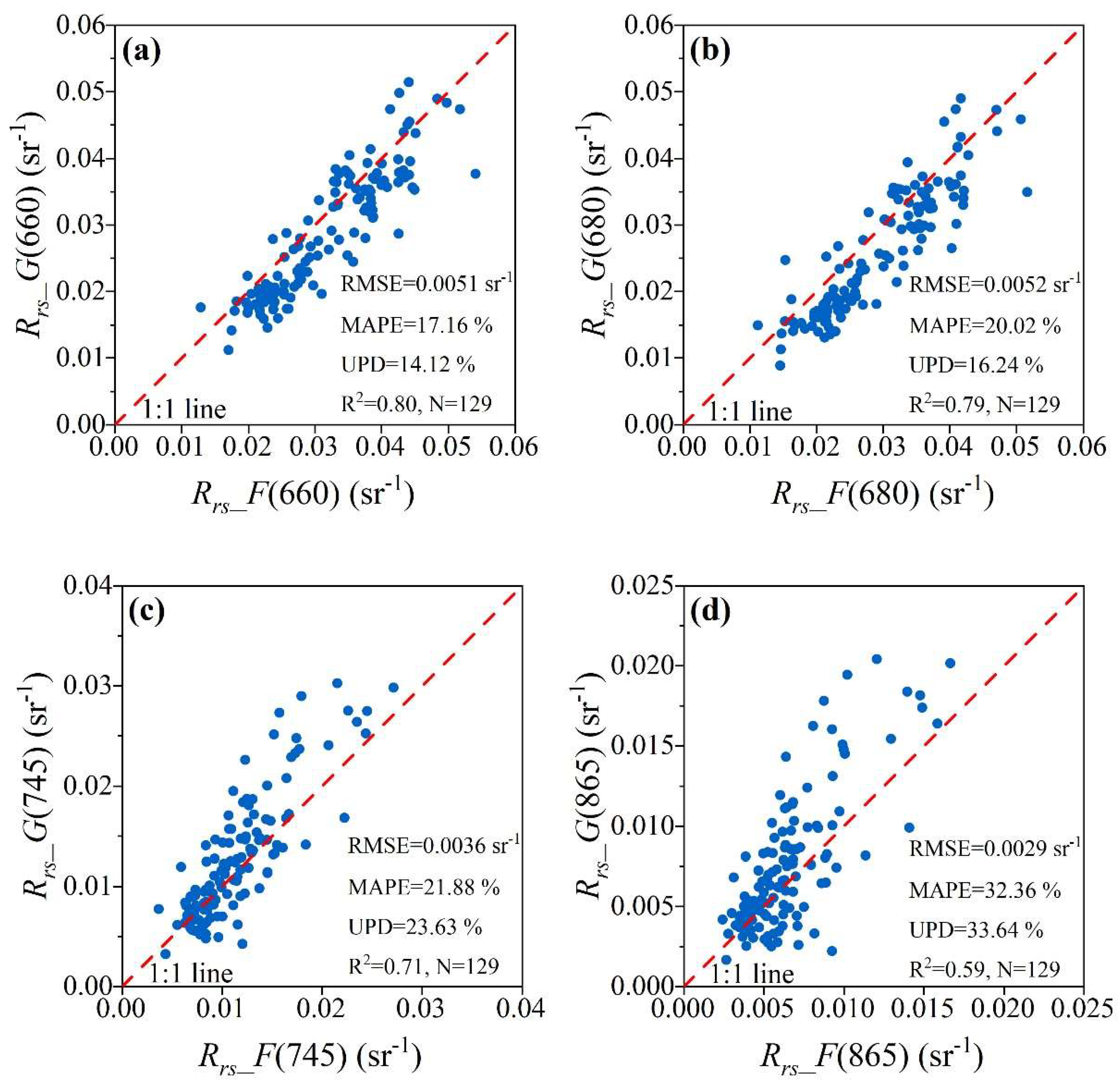
A total of 4249 high-quality GOCI images were finally selected according to the above rules. There are 129 match-up pairs between the field measurements and GOCI data obtained to evaluate the atmospheric correction accuracy. GOCI R_rs_G at 660, 680, 745, and 865 nm bands were validated with the in situ R_rs_F in Figure 4. The R² values of the four bands were greater than 0.59, indicating good performance.

2.4. Meteorological and Hydrological Data

Data on the hourly WIN over Lake Chaohu from 2011 to 2020 were downloaded from the European center for Medium-Range Weather Forecasts (ECMWF) ERA5 dataset. This dataset has a horizontal grid resolution of 0.25°, corresponding to around 31 km [48]. Data on the hourly global horizontal irradiance (GHI) from 2011 to 2020 in Lake Chaohu were downloaded from the National Solar Radiation Database (NSRDB), with a spatial resolution of 4 km. Digital elevation model (DEM) data of Lake Chaohu with a spatial resolution of 30 m were obtained from the Lake-Watershed Science Data Center, National Earth System Science Data Sharing Infrastructure, National Science & Technology Infrastructure of China (http://lake.geodata.cn, accessed on 1 January 2024), and resampled to 500 m. The daily water level data of Lake Chaohu were obtained from the Hydrological Bureau of Anhui Province. The water depth (m) data were obtained by subtracting the water level from the DEM data.

2.5. Accuracy Assessment

Four statistical metrics were used to evaluate model performance: the coefficient of determination (R²), root mean square error (RMSE), mean absolute percentage error (MAPE), and unbiased percentage difference (UPD). The coefficient of variation (CV) was used as a statistic for sample screening and model validation. These metrics are defined as follows:

$$\mathrm{RMSE}=\sqrt{{\displaystyle \frac{1}{N}}{\displaystyle \sum _{i=1}^N{(X_i-Y_i)}^2}},$$

(3)

$$\mathrm{MAPE}={\displaystyle \frac{1}{N}}{\displaystyle \sum _{i=1}^N\frac{|X_i-Y_i|}{X_i}}\times 100\%,$$

(4)

$$\mathrm{UPD}={\displaystyle \frac{1}{N}}{\displaystyle \sum _{i=1}^N\frac{|X_i-Y_i|}{X_i+Y_i}}\times 200\%,\mathrm{and}$$

(5)

$$\mathrm{CV}={\displaystyle \frac{\sqrt{{\displaystyle \sum _{j=1}^N{(R_j-\overline{R})}^2/N}}}{\overline{R}}}\times 100\%,$$

(6)

where N is the number of samples, X_i and Y_i are the corresponding values at point i, R_j is the value of j in a 3 × 3 window, and $\overline{R}$ is the mean value within the window.

3. Methods

3.1. Fitting the Chla Vertical Profiles Using Field-Measured Data

For the 224 field measured data, we used an approach from the literature [36]: When the CV of the Chla vertical profiles was less than 20%, the vertical profile was classified as vertically uniform (Type 1). Otherwise, the vertical profile was classified as vertically non-uniform (Type 2).

From the previous research, five models (Chla(z) = a × exp(b × z) + c, Chla(z) = a₂ × exp(b₂ × z + c₂), Chla(z) = a₃ × exp(b₃ × z), Chla(z) = a₄ × z^b4 + c₄, and Chla(z) = a₅ × z^b5) were selected to fit the vertical profiles of Type 2. The function with the best fitting performance was used to describe the Chla(z). The key steps in the following sections were to estimate the vertical structure parameters of the Chla(z) fitting function using R_rs_G and environmental factors.

3.2. Correlation of Surface Chla with R_rs_G

Referring to the previous Chla inversion model, AFAI_Rrs [49], normalized difference vegetation index (NDVI) [50], fluorescence line height (FLH) [51], spectral index (SI) [52], and X [53] calculated from R_rs_G were used as exponential factors to invert the Chla model, and the calculation methods are shown in Equations (7)–(11):

$${\mathrm{AFAI}}_{R_{rs}}=R_{rs}(745)-R_{rs}(660)-((R_{rs}(865)-R_{rs}(660))\times {\displaystyle \frac{745-660}{865-660}}),$$

(7)

$$\mathrm{FLH}=R_{rs}(680)-R_{rs}(660)-((R_{rs}(745)-R_{rs}(660))\times {\displaystyle \frac{680-660}{745-660}}),$$

(8)

$$\mathrm{NDVI}={\displaystyle \frac{R_{rs}(745)-R_{rs}(660)}{R_{rs}(745)+R_{rs}(660)}},$$

(9)

$$\mathrm{SI}={\displaystyle \frac{\exp \left(R_{rs}(660)\right)-\exp \left(R_{rs}(865)\right)}{\exp \left(R_{rs}(660)\right)+\exp \left(R_{rs}(865)\right)}},\mathrm{and}$$

(10)

$$\mathrm{X}=\left({\displaystyle \frac{1}{R_{r\mathrm{s}}(660)}}-{\displaystyle \frac{1}{R_{r\mathrm{s}}(680)}}\right)\times R_{rs}(745).$$

(11)

Based on the 129 match-up pairs between the field data and GOCI measurements, R_rs_G of each band were extracted, from which index factors were calculated. In previous studies, it was reported that R_rs at B5 and B8 bands were more related to Chla estimation. Therefore, we correlated the B5–B8 and index factors of R_rs_G with the measured Chla(surface) in

Table 1. Correlations between different factors and the measured Chla(surface) (r is the Pearson correlation coefficient). R_rs single-band factors and Chla(surface) (first two columns), index factor and Chla(surface) (columns 3 and 4), and index factor and Chla(surface) (columns 5 and 6).

Single-Band Factor	r	Index Factor	r	Index Factor	r
B5 (660 nm)	−0.34	AFAIRrs (B7, B5, B8)	0.67	NDVI (B7, B5)	0.66
B6 (680 nm)	−0.44	FLH (B6, B5, B7)	−0.51	B8/B7 (B8, B7)	0.17
B7 (745 nm)	0.27	SI (B5, B8)	−0.55	WIN	−0.45
B8 (865 nm)	0.26	X (B5, B6, B7)	−0.41

.

3.3. Decision Tree for Classifying Vertical Profiles

To better invert Chla(z) and analyze the patterns of vertical profiles, we needed to build a decision tree to classify the vertical profiles. For the 129 match-up pairs between field measurements and GOCI image data, we found the index factors (AFAI_Rrs, SI, FLH, NDVI, WIN) with good correlations (as shown in Table 1), which were selected as parameters for Chla(z) classification. These index factors were used as nodes of the tree to obtain the best classification results by setting different thresholds. A decision tree was established to classify Chla(z), using R_rs_G and WIN.

We used ten-fold cross validation to estimate the decision tree classification accuracy, where the data were divided into 10 equally (or nearly equally); training and validation were each performed 10 times, with one dataset reserved for validation and the remaining nine for training in each iteration [54]. Classification accuracy was assessed using an error matrix, where the resulting classification classes were compared with measured data. From the error matrix, overall accuracy, Kappa coefficient, user’s accuracy, and producer’s accuracy were calculated [36].

3.4. Chla(z) Inversion Model Development

We propose a method (Figure S1) for inverting Chla(z) using the R_rs_G, index factors and meteorological data. The Chla(z) profiles were fitted to select a model with good performance using field-measured data. Then, the index factors of R_rs_G were calculated, and the correlations between the index factors and Chla(surface) were analyzed. For the 129 match-up pairs between the field and GOCI data, we selected the variables as parameters for Chla(z) classification. A decision tree was established to classify Chla(z), using R_rs_G and WIN. Then, Chla(z) profiles were classified as Type 1 or Type 2.

For Type 1 Chla(z), we used Guo et al. model [45] to estimate Chla. For Type 2 Chla(z), we estimated the three vertical parameters (a, b, and c) in the equation. Then, we used a multiple regression model (y = m × x₁ + n × x₂ + l × x₃ + p × x₄ + k, where m, n, l, p, and k are constants) to invert parameters a, b, and c. To avoid overfitting the data (36 match-up pairs between measured data and GOCI data), the coefficients of the multiple regression model were calculated via Python using the Ten-fold crossover method, with 80% serving as a training data set and 20% serving as a test data set. After obtaining the three vertical parameters, the Type 2 Chla(z) inversion model was obtained, and Chla(z) values were calculated using the new Type 2 Chla(z) model for each pixel.

4. Results

4.1. Fitting of the Field Chla(z) Profiles

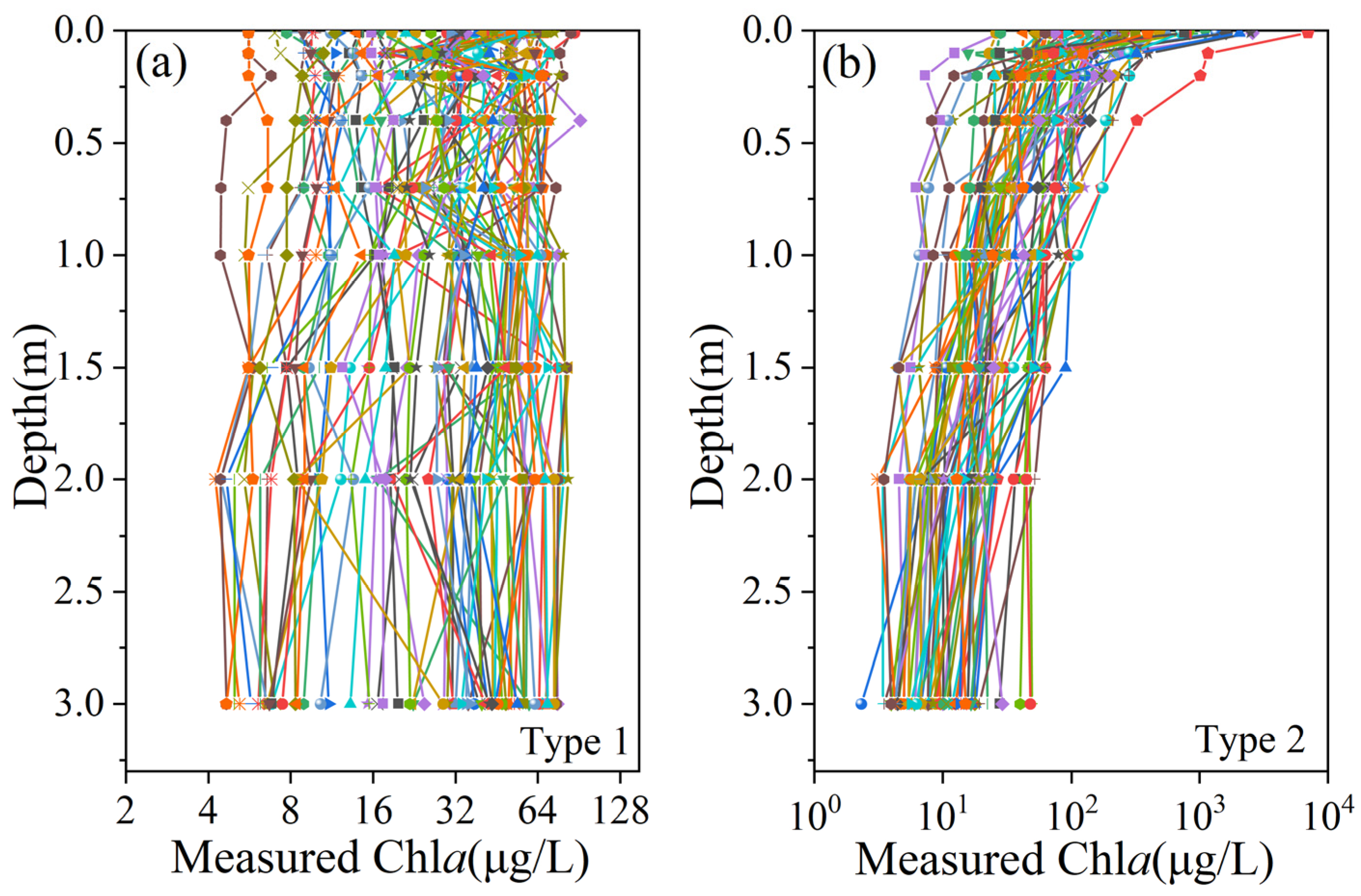
According to the CVs of the measured 224 Chla(z) profiles, 166 Chla(z) profiles were classified as Type 1 (CV < 20%), and 58 Chla(z) profiles were classified as Type 2 (CV > 20%), as shown in Figure 5. For the Type 2 Chla(z) profiles (58 samples), the results of the predicted Chla(z) and measured Chla(z) from the fitted models are shown in

Table 2. Results of the predicted Chla(z) and measured Chla(z) from the fitted models. The models with better performance are noted in bold (z is water depth).

Name	Function	R²	RMSE (μg/L)	UPD (%)	MAPE (%)
Model 1	Chla(z) = a × exp(b × z) + c	0.98	38.15	23.03	17.15
Model 2	Chla(z) = a2 × exp(b2 × z + c2)	0.97	45.15	29.28	20.05
Model 3	Chla(z) = a3 × exp(b3 × z)	0.97	45.43	27.60	21.00
Model 4	Chla(z) = a4 × zb4 + c4	0.92	96.28	51.35	37.41
Model 5	Chla(z) = a5 × zb5	0.97	38.08	26.44	21.14

. Model 1, which had high R² values and low RMSE, UPD, and MAPE values, was selected as the best-fitting model. The corresponding parameters a, b, and c for Type 2 Chla(z) were obtained based on Model 1, wherein the range of coefficient a was between 0 and 1500, with an average of 398.03; the span of b ranged from −20 to 0, with an average of −6.93; and the range of c was between 20 and 40, with a mean of 29.36.

4.2. Calibration and Validation of Chla(z)

4.2.1. Decision Tree of Chla(z)

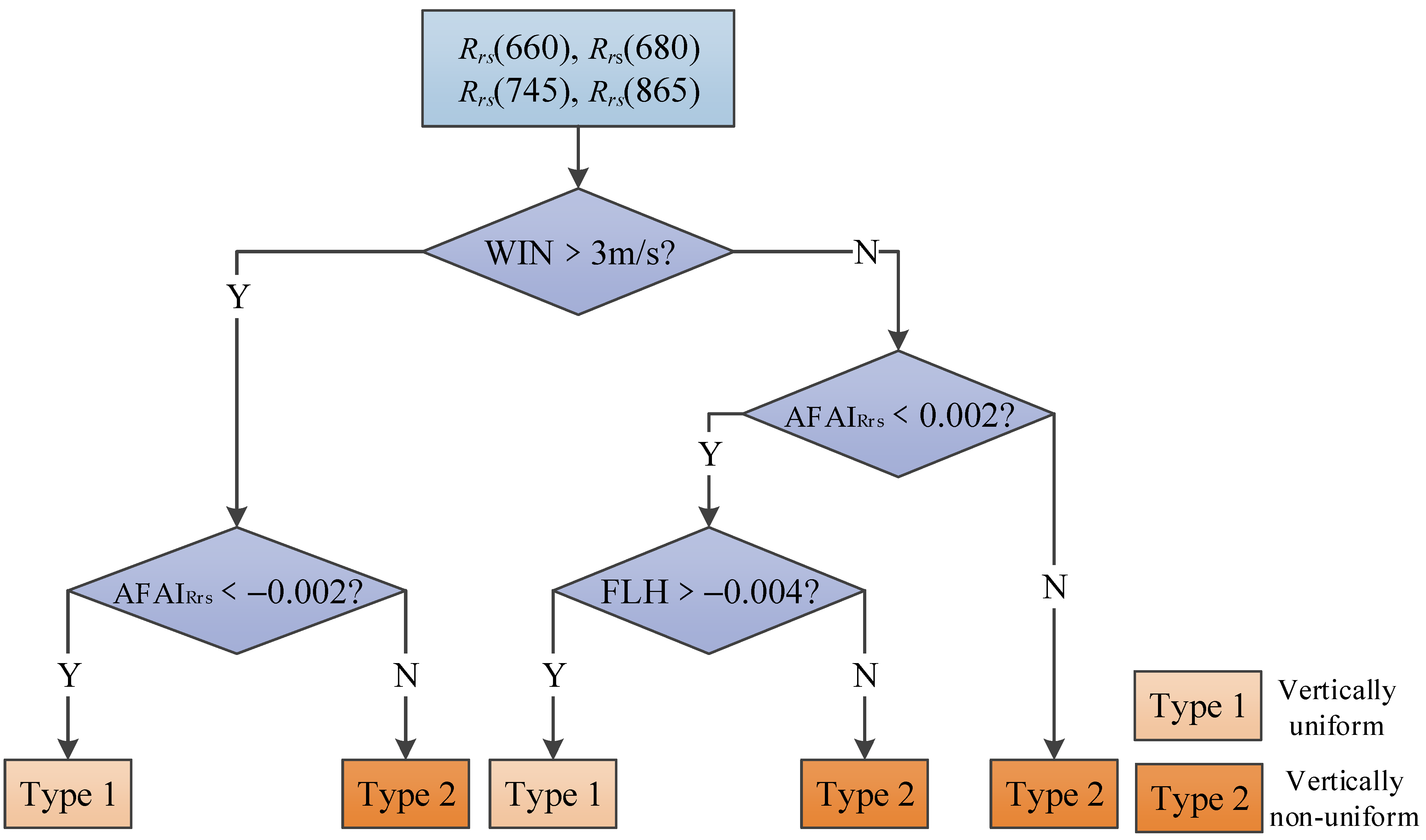
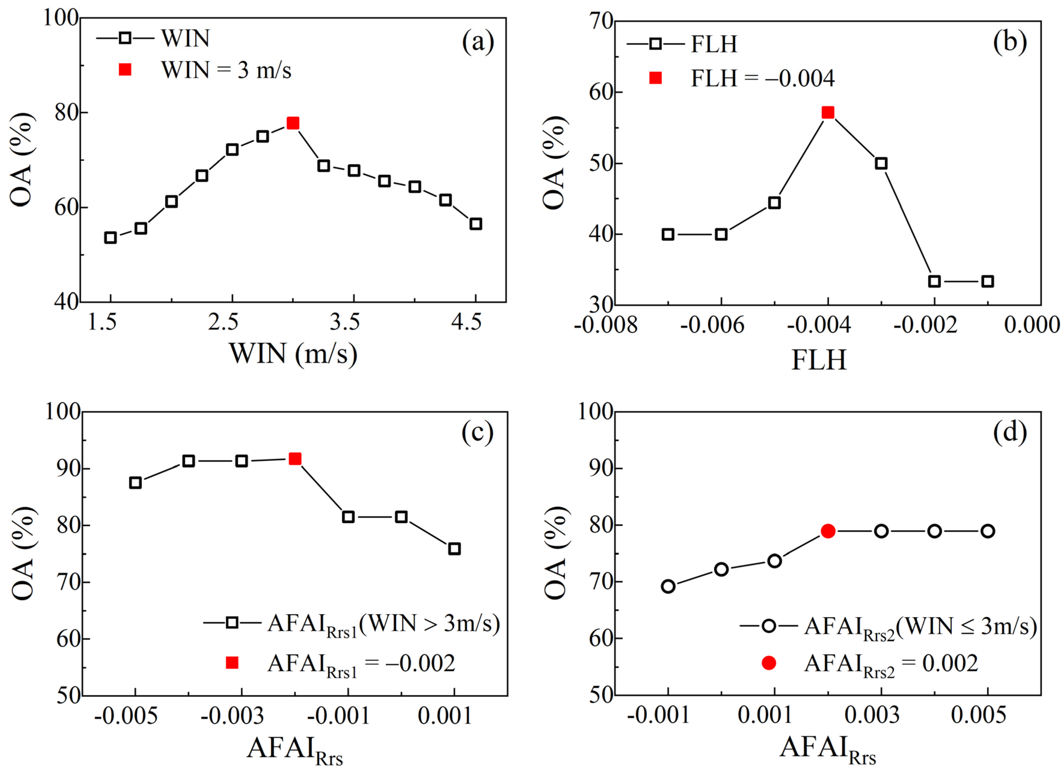
A decision tree of the Chla(z) vertical profiles was established using R_{rs_}G and WIN (Figure 6). The cases wherein (1) WIN > 3 m/s and AFAI < −0.002 or (2) WIN ≤ 3 m/s, AFAI < 0.002, and FLH > −0.004 belonged to Type 1, and the rest of the cases belonged to Type 2. The classification results followed an error matrix, with the numbers on the diagonal being correct classifications. The classification accuracy of the decision tree was assessed using the ten-fold cross validation method (

Table 3. Error matrix for Chla(z) classes of Lake Chaohu (68 randomly selected sample points), where “Overall Accuracy” is the overall accuracy of validation, and “Kappa” is the Kappa coefficient.

		Measured Class			User’s Accuracy
		Type 1	Type 2	Total
Predicted class	Type 1	28	5	33	85%
	Type 2	2	33	35	94%
	Total	30	38	68
Producer’s Accuracy		93%	87%
Overall Accuracy		89%		Kappa	0.79

), wherein the overall accuracy was 89% and the Kappa coefficient was 0.79. The thresholds for the decision tree were assessed, showing that WIN, AFAI_Rrs, and FLH in the decision tree were measured with the highest accuracy (Figure 7).

4.2.2. Chla Inversion Model for Vertically Uniform

According to the Pearson correlation values in Table 1, AFAI_Rrs was chosen to construct the Type 1 inversion model.

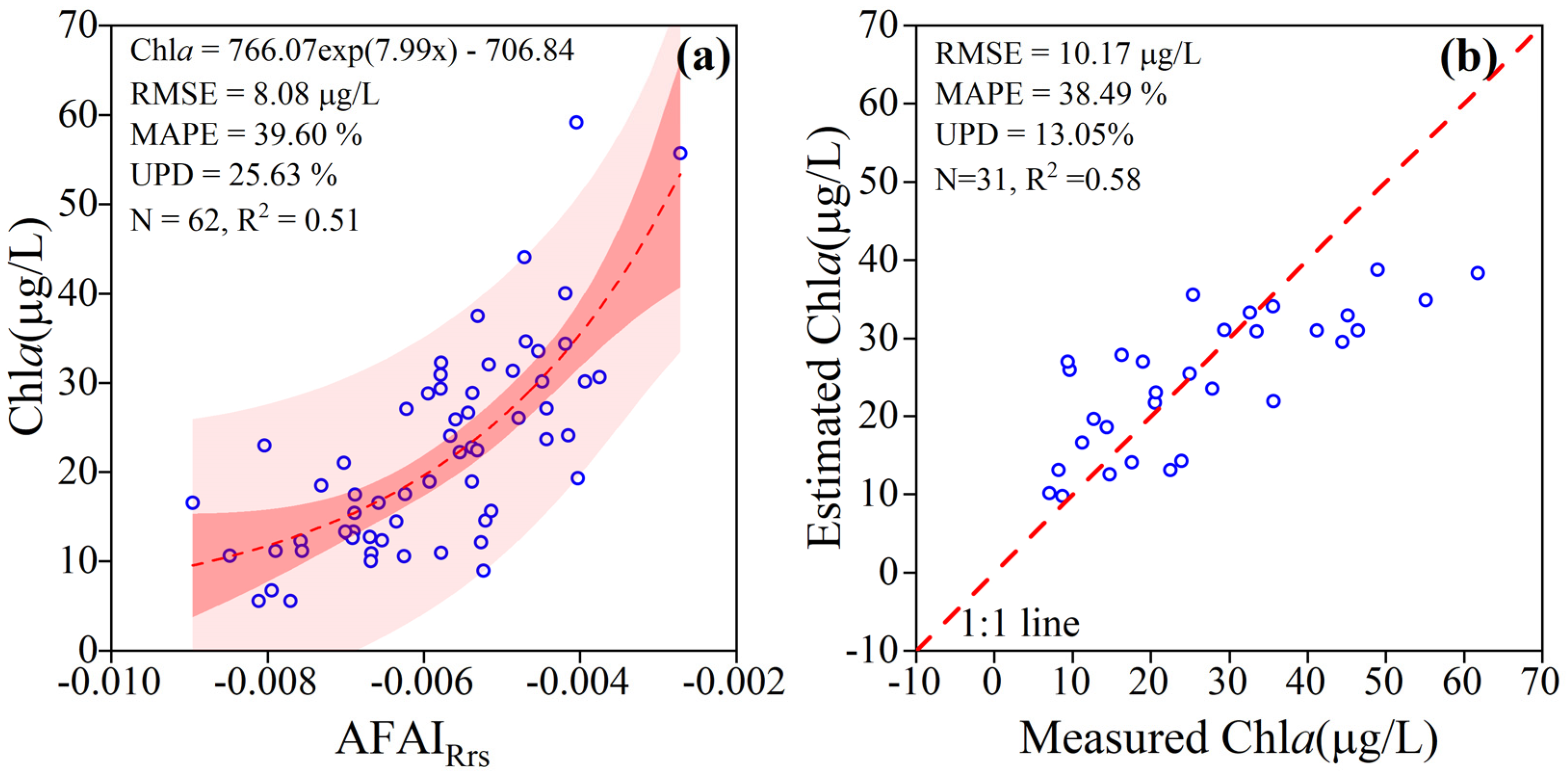
There were 93 match-up pairs between the field and GOCI data in Type 1, which were randomly sorted to generate a random array, with one out of every three samples serving as a validation set. Sixty-two samples were used for model training, and thirty-one samples were used for validation. The Type 1 inversion model was Chla = 766.07 × exp (7.99 × x) − 706.84 (Figure 8), where x is AFAI_Rrs, with the training data R² = 0.51 and the validation data R² = 0.58. For Lake Chaohu, the AFAI_Rrs–Chla model was able to estimate Chla reasonably well when the vertical distribution of the water column was uniform.

4.2.3. Estimation of Chla(z) Inversion Model in the Non-Uniform Vertical Distribution

Due to weather conditions, solar angle, and the quality of GOCI images, only 36 match-up non-uniform samples were used for Chla(z) validation. A correlation analysis was conducted between single-band data, meteorological data (GHI, wind speed, temperature), and index factors in the Chla inversion models with the vertical structural parameters in Figure 9. It showed that B86, AFAI_Rrs, WIN, GHI, and X have good relationships with the vertical structural parameters. The validation results regarding vertical non-uniformity (36 samples) between the field data and predicted data are presented in Figure S2. After calculating the coefficients of the multiple regression models using Python, the three structural parameters were estimated using Equations (12)-(14). The training results for three structural parameters were as follows: a: R² = 0.54, RMSE = 286.26; b: R² = 0.46, RMSE = 6.90; c: R² = 0.20, RMSE = 17.19; the validation results are shown in Figure 10a–c (a: R² = 0.57, RMSE = 270.67; b: R² = 0.56, RMSE = 6.67; c: R² = 0.38, RMSE = 16.33). A total of 324 match-up pairs (36 samples, nine layers) were used to validate the model (R² = 0.75, RMSE = 72.80 μg/L), as shown in Figure 10d.

$$a=0.83\times GHI-26862.04\times AFAI+1175.93\times B86-123.63\times WIN+487.58$$

(12)

$$b=-0.01\times GHI+833.57\times AFAI-34.04\times B86+2.89\times WIN-18.69$$

(13)

$$c=0.04\times GHI-76.59\times X-22.58\times B86-3.38\times WIN-2.55$$

(14)

4.3. Temporal and Spatial Variations in Chla(z)

4.3.1. Interannual Variation in Chla(z)

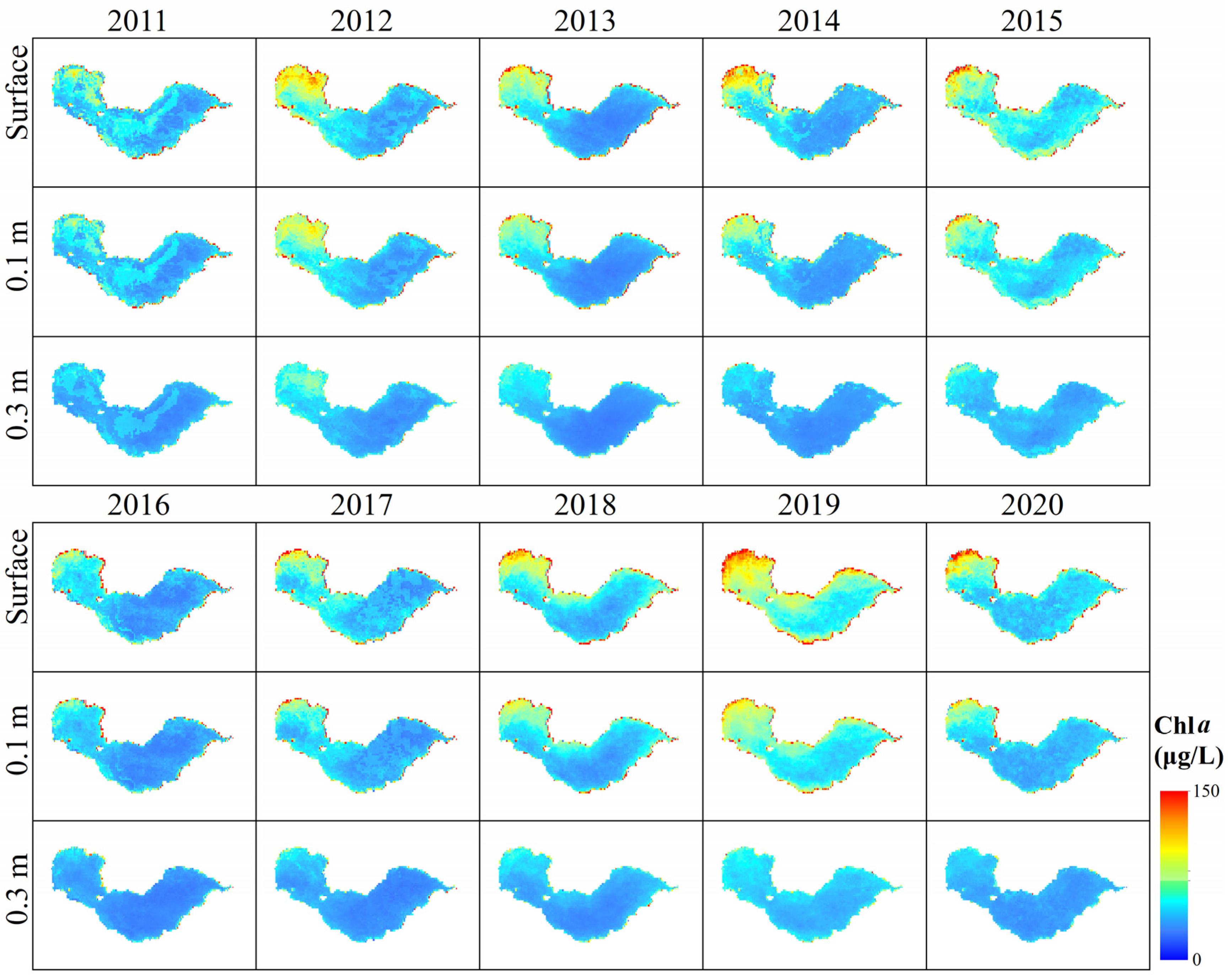
The annual average Chla of the above three layers (z = surface, 0.1, and 0.3 m) from 2011 to 2020 is illustrated in Figure 11. According to the mean values of all GOCI data from 2011 to 2020, the highest Chla (55.47 ± 28.36 μg/L) was found in the surface layer, while Chla were 47.85 ± 20.57 μg/L and 36.28 ± 8.60 μg/L at 0.1 m and 0.3 m, respectively. The mean surface Chla was the highest in 2019, reaching 76.81 μg/L. In 2016, the mean Chla was the lowest, at only 45.67 μg/L. The mean vertical Chla in other layers remained consistent with that of the surface. In the 2011–2015 period, the average Chla(z) value had a small peak in 2012 and then increased from 2013 to 2015, with a secondary peak in 2015 (61.18 μg/L), while the average Chla(z) decreased to the lowest value in 2016, and from 2017 to 2020, the average Chla(z) increased again, reaching a maximum, and then declined. The annual average values of Chla(z) at 0.1 and 0.3 m had a trend similar to that of the surface Chla. There were significant differences in the mean Chla(z) values among the different years, but overall, the Chla(z) values in the western part of Lake Chaohu were greater than those in the eastern part.

4.3.2. Monthly Variation in Chla(z)

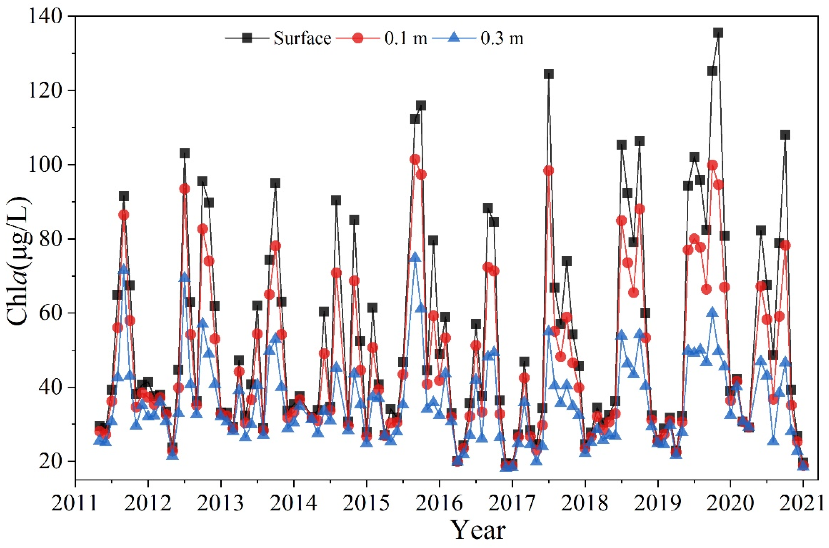
The variation in the monthly average Chla(z) (where z = surface, 0.1 m, and 0.3 m) from 2011 to 2020 is shown in Figure 12. The Chla(z) in each layer showed seasonal changes that were high in summer and low in winter. Chla(z) (where z = surface) values were the highest in summer (from June to August), reaching 75.10 μg/L, and the lowest in winter (December to February of the following year), at only 36.38 μg/L.

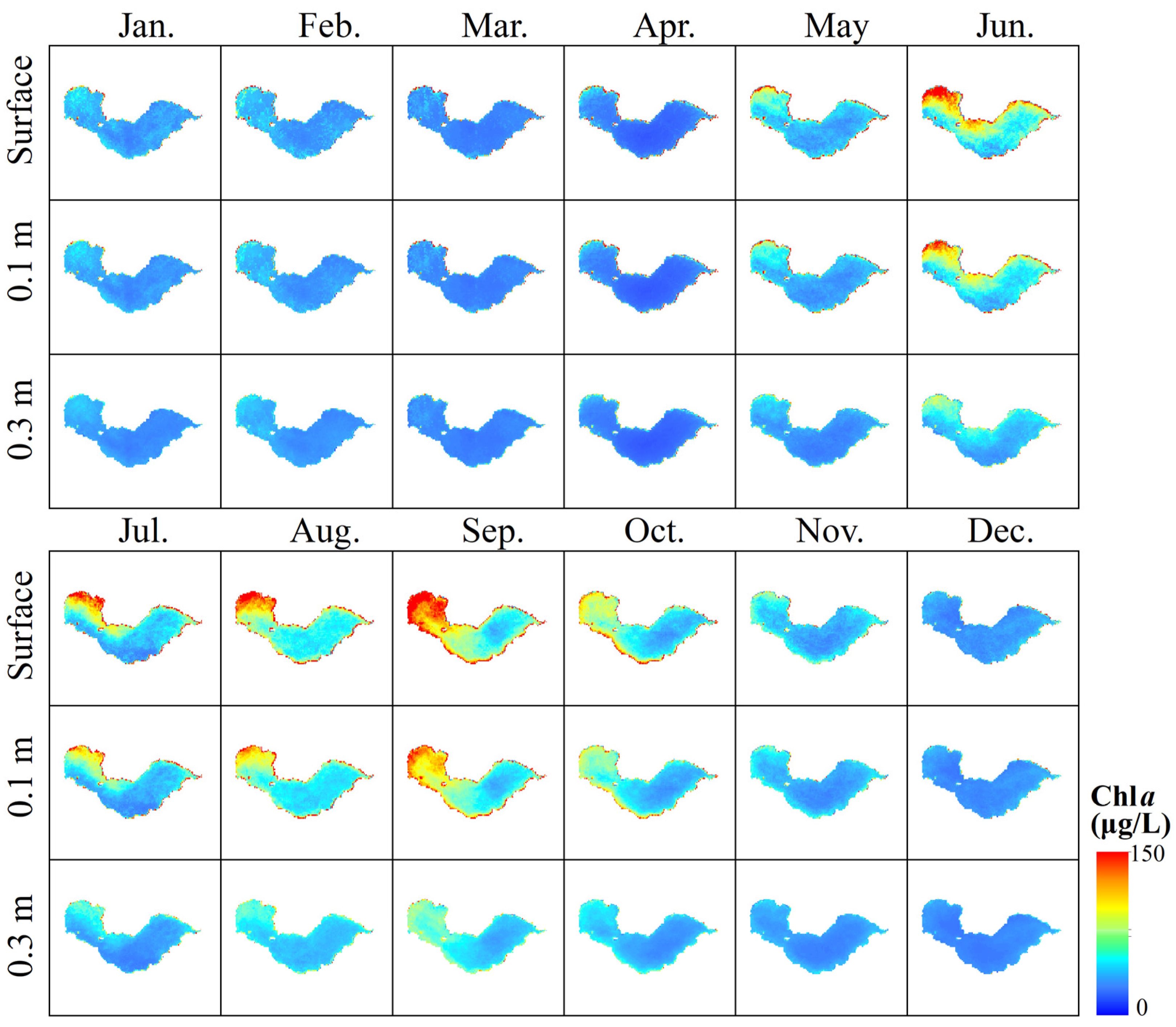
The monthly spatial distribution of Chla(z) (Figure 13) showed that the highest mean value of surface Chla(z) (95.86 μg/L) was recorded in September, followed by the second highest value in August (79.17 μg/L), and lower mean values were in December (32.95 μg/L) and April (32.62 μg/L). The lowest value for the whole year was recorded in March (32.24 μg/L). The trend of the monthly mean Chla values at z = 0.1 and 0.3 m was also similar to that of the surface layer. From the overall inter-monthly trend, the monthly mean Chla(z) reached its maximum in September and gradually decreased from October onward. However, vertical inhomogeneity of Chla was not observed in the winter or early spring.

4.3.3. Diurnal Variations in Chla(z)

The diurnal mean Chla(z) for all the GOCI images from 2011 to 2020 showed significantly vertical variations (Figure 14). In terms of surface Chla, (1) Chla values were the lowest from 8:16 to 10:16, with a mean value of 42.02 μg/L, and highest values were mainly found near the western and the southeastern parts of the lake; (2) there was an overall increase from 11:16 to 13:16, with a maximum mean value of 54.06 μg/L reached at 12:16; and (3) there was a gradual decrease in Chla from 13:16 to 15:16, with a mean value of 47.21 μg/L. From a perspective of vertical Chla distribution, the mean Chla in the surface layer fluctuated significantly within a day, while the change decreased with an increasing water depth. The structural parameters a and c first increased and then decreased, while the trend of b was the opposite, first decreasing and then slightly increasing. The structural parameters a and c were higher, and b was lower, at 11:16, while the vertical direction of the corresponding moments at this time showed large differences. Parameters a and c were basically the same as Chla (same units), which gradually increased from 8:16 to a peak at approximately 12:16 and then gradually decreased.

4.4. Dynamics of the Vertical Structural Parameters

The spatial distributions of the mean values of the vertical model structural parameters (a, b, and c) are shown in Figure 15. The mean values had more obvious spatial differences: the mean value of parameter a was greater in the central lake area, while the mean value of parameter b was greater in the western lake area. Model parameter a reached a maximum value of 463.53 in the spring (March–May), a minimum of 349.66 in the winter, 424.96 in the summer, and 368.12 in the autumn (September–November). Model parameter c had the same seasonal trend as the value of parameter a, both of which had a maximum (34.52) in the spring and a minimum (22.63) in the winter.

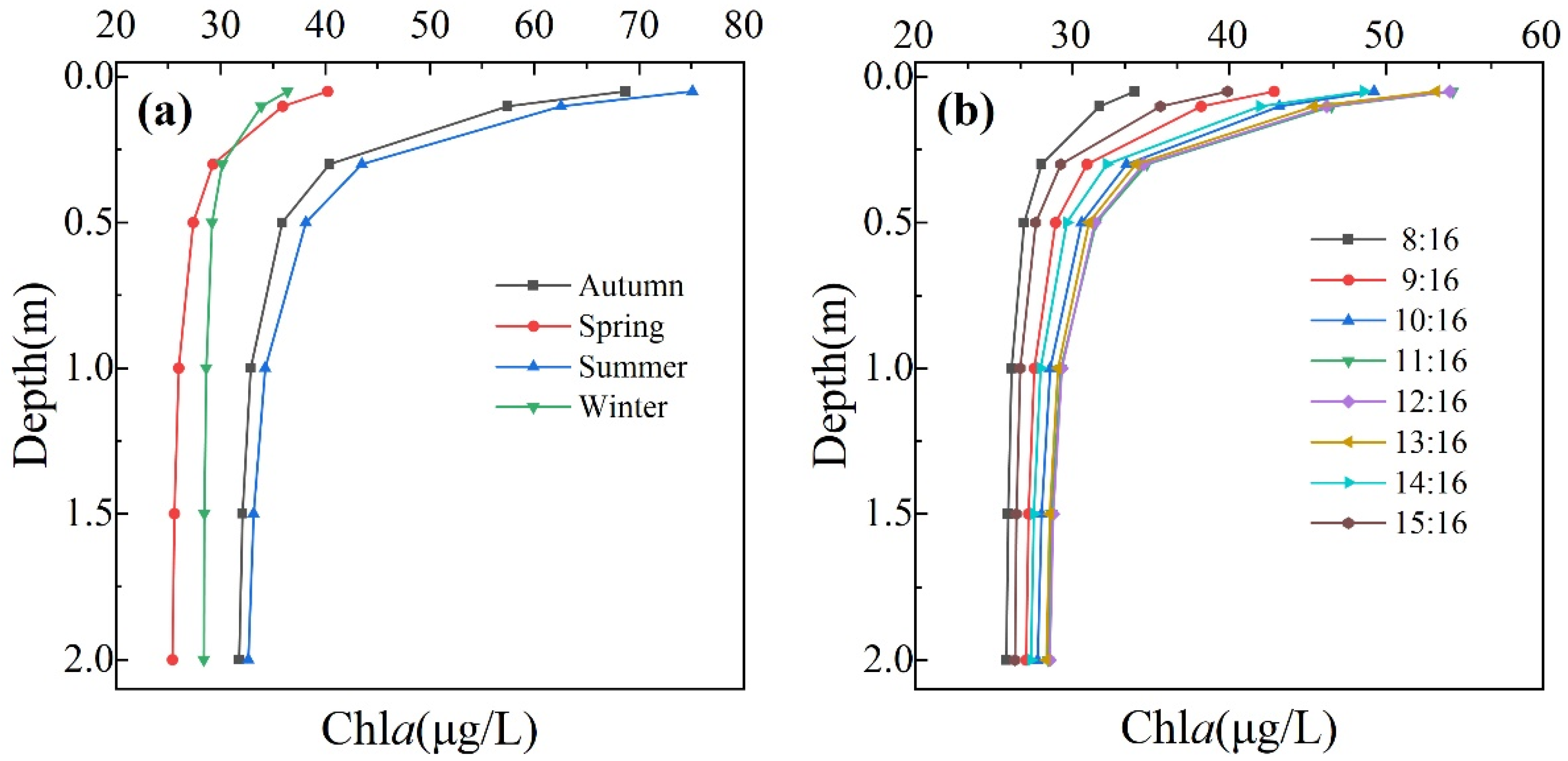
The seasonal and diurnal variations in Chla(z) are illustrated in Figure 16. The curve depicting Chla(z) was the steepest during the summer. The range of variation in Chla(z) in Lake Chaohu was significantly larger in the summer and autumn than in the spring and winter. In fact, the average rates of change in Chla(z) in the spring, summer, autumn, and winter were 14.95, 43.95, 38.09, and 8.31 μg/L·m⁻¹, respectively. The mean vertical Chla varied greatly from the surface to 0.5 m. The average rates of change in Chla at 0, 0.1, 0.2, 0.3, 0.4, and 0.5 m were 76.48, 58.03, 15.96, 4.43, 1.22, and 0.53 μg/L·m⁻¹, respectively. When the depth was greater than 0.5 m, the mean Chla remained at a certain concentration (25.73 μg/L) and no longer fluctuated. During the 8 h period from 8:16 to 15:16, the mean Chla(z) in Lake Chaohu was more variable from 11:16 to 13:16. The Chla average rates of change in diurnal variations from 8:16 to 15:16 were 9.69, 19.20, 25.64, 31.52, 31.49, 30.81, 26.32, and 16.96 μg/L·m⁻¹, respectively.

5. Discussion

5.1. Advantages of the Proposed Chla(z) Inversion Model

Herein, an exponential function of Chla(z) is proposed to quantitatively characterize the vertically non-uniformly distributed Chla values. By comparing the existing types, the exponential vertical distribution function proposed in this paper can fit Chla(z) well, with a reduced number of structural parameters. In addition, WIN and wave current affect the horizontal and vertical movement of phytoplankton, and algae aggregate near the water surface in certain conditions with low WIN [25,55]. Light is an important energy source required by algae to carry out photosynthesis, which has a direct effect on their vertical movement in the water column [38]. Therefore, using hourly WIN and light as input parameters to estimate the structural parameters can improve model performance.

The spatial and temporal dynamics of algal biomass under non-algal bloom conditions in Lake Chaohu were investigated using the baseline normalized difference bloom index (BNDBI) of MODIS data [56]. The Algal Biomass Index (ABI) was developed based on MODIS data to estimate the total algal biomass of Lake Chaohu [57]. However, the cited authors established the relationship between remote sensing signals and the total algal biomass directly, ignoring the vertical distribution of Chla of each pixel. In addition, due to the high temporal resolution of GOCI data, they can reflect the diurnal changes in Chla in the vertical profiles.

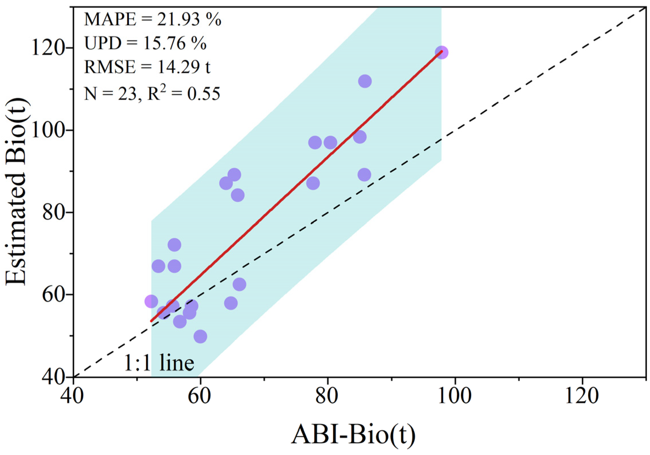
We used 11 match-up pairs of MODIS and GOCI within ± 0.5 h to compare their performance in estimating algal biomass within the water column. The ABI algorithm was used to calculate the total algal biomass of the whole lake (ABI-Bio) [57], and the total algal biomass in this study was obtained by integrating the vertical Chla of each pixel (Estimated-Bio) (Figure 17). The result indicated the existence of a linear relationship (R² = 0.47) between ABI-Bio and Estimated-Bio, with an RMSE = 14.89 t. Note that the ABI-Bio-algorithm-derived value was relatively low in conditions with total algal biomass > 80 t, in which the floating algal blooms were masked in the ABI-Bio algorithm. In addition, the total algal biomass estimated in this study is theoretically a more accurate estimation and, to a certain extent, reflects the phytoplankton distribution in three dimensions, which helps to capture the dynamics of Chla in horizontal and vertical directions with high resolution. The vertical distribution of Chla(z) in different layers is shown in Figure 18.

5.2. Drivers of Diurnal Variation in Chla(z)

According to the intraday distribution of Chla(z) in Lake Chaohu, Chla increased from 8:16 to 13:16 and then decreased from 13:16 to 15:16, which was consistent with the trend in which algal blooms tend to increase and then decrease over one day under the combined effects of light and WIN [49]. There were significant spatial differences in Chla(z) in Lake Chaohu, but the western part of Lake Chaohu had larger Chla(z) values than those in other parts of the lake [58].

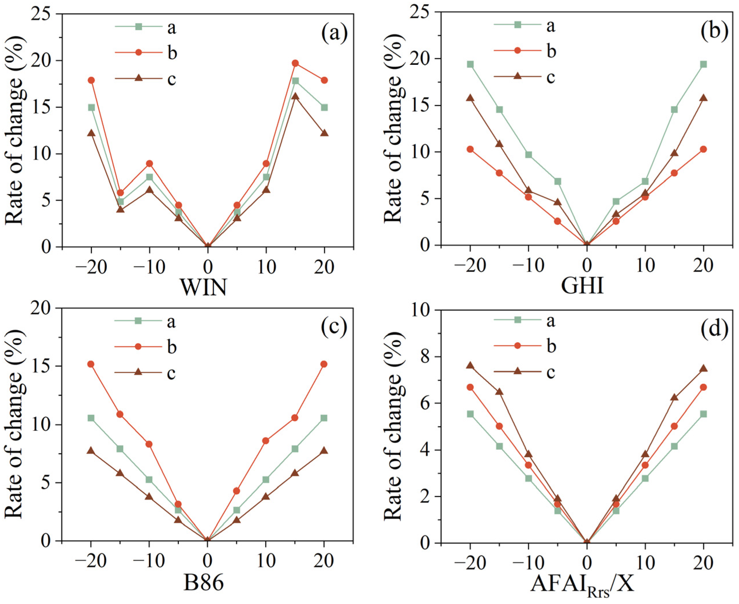
The annual mean Chla(z) increased in 2014 due to the increase in mean annual temperature and increase in nutrient inputs of nitrogen and phosphorus, and this trend was consistent with the trend of the risk level of cyanobacteria blooms in Lake Chaohu [58]. Due to the lower mean annual WIN and greater light intensity in 2019, Chla(z) had a peak in this year, which was consistent with a previous study [45]. Considering the effect of wind speed, GHI, etc., on the structural parameters, a sensitivity analysis was conducted (Figure 19). It indicated that the parameters a and c were sensitive to GHI (with a rate of change in a < 20% and rate of change in c < 17%), the parameter b was sensitive to WIN (rate of change < 20%), and the parameters a, b, and c were insensitive to AFAI_Rrs/X.

5.3. Uncertainties and Limitations

Due to differences in the sampling times between the field-measured and satellite-obtained data and the problem of mixed pixels, there are limitations in the prediction accuracy in the Type 1 model. If there are enough samples, we also recommend using the Random Forest approach to calculate Chla. The model-derived structural parameters for Type 2 were approximately the same as the spatial and temporal variations in Chla. But the value of structural parameter a was not linearly correlated with Chla, which reached a maximum value when a was approximately 400 and then decreased as parameter a increased. As the inversion model of structural parameters involves multiple input factors, the complexity and uncertainty of the model will increase. Therefore, the range of surface Chla applied in this study was 0–500 μg/L. When Chla was greater than 500 μg/L, the function needed to be tuned using local measured data. In addition, although we used the ten-fold cross validation method to validate the model, the performance of the model still could not reach the high accuracy expected due to the limited number of samples. An increase in the number of samples will improve this model’s performance.

Satellite data with different spatial resolutions can have an impact on the results of algal bloom extraction and water color parameter inversion, and a 500 m spatial resolution of GOCI may not detect more details in spatial variations of Chla. Although the atmospheric correction method used in this study is more rigorous, the spatial and temporal variations in atmospheric conditions and the uncertainty of observation conditions affect the accuracy and reliability of the inversion results of Chla [31,59]. In addition, the surface features at the land-water interface are highly variable, which may give rise to a mixed image problem in remote sensing observations [60]. These mixed image problems are highly likely to lead to the misidentification of cyanobacteria blooms or aquatic vegetation, which result in high Chla at the boundary of Lake Chaohu [61,62]. GOCI-II can provide observation data from 2021 to the present, with a higher spatial resolution (250 m) and more spectral wavelengths, and these data are more applicable for the near-real-time monitoring of inland water bodies.

In this study, we assumed that all in situ data (vertical distributions) could be well represented for the entire lake and then combined the GOCI data (only on surface/integrated top layer information, constructing the GOCI data surface–verticality relationship) to invert the distribution of Chla in the lake. However, this assumption may not be true for other lakes. In addition, the environmental factors used in this study are WIN and GHI in Lake Chaohu, but their spatial differences were not considered. In addition to WIN and light, water temperature has a significant effect on the increase in algal biomass, but it is more related to the seasonal and annual variations of phytoplankton in Lake Chaohu [60,63]. Therefore, environmental factors related to the Chla vertical distribution may differ with varying natural conditions [38,52], while environmental factors with high spatial resolutions will improve the estimation of Chla vertical profiles.

6. Conclusions

An exponential model was proposed to simplify the types of Chla vertical profiles using the fitting of the in situ-measured Chla data in Lake Chaohu. A decision tree was constructed using AFAI_Rrs, FLH, and WIN. The Chla vertical profiles were classified into two types (vertically uniform and vertically non-uniform), where the overall accuracy of classification was 89% with a Kappa coefficient of 0.79. The results showed that the model-derived Chla(z) had a significant correlation with the measured Chla(z) (R² = 0.68), indicating that the Chla(z) estimation using the non-uniform vertical distribution model in Lake Chaohu was reasonable. In addition, the spatial and temporal variations in the vertical profiles of Chla(z) in Lake Chaohu from 2011 to 2020 were illustrated, providing a useful tool for assessing the effectiveness of phytoplankton bloom management and treatment in lakes. We believe that the strategy of combing R_rs_G and environment factors in a Chla(z) inversion model has the potential to be extended to other eutrophic lakes.

References

1. Jiang, Y.; He, W.; Liu, W.; Qin, N.; Ouyang, H.; Wang, Q.; Kong, X.; He, Q.; Yang, C.; Yang, B.; et al. The seasonal and spatial variations of phytoplankton community and their correlation with environmental factors in a large eutrophic Chinese lake (Lake Chaohu). Ecol. Indic. 2014, 40, 58–67. [Google Scholar] [CrossRef]
2. Wang, Y.; Guo, Y.; Zhao, Y.; Wang, L.; Chen, Y.; Yang, L. Spatiotemporal heterogeneities and driving factors of water quality and trophic state of a typical urban shallow lake (Taihu, China). Environ. Sci. Pollut. Res. 2022, 29, 53831–53843. [Google Scholar] [CrossRef] [PubMed]
3. Le, C.; Hu, C.; English, D.; Cannizzaro, J.; Kovach, C. Climate-driven chlorophyll-a changes in a turbid estuary: Observations from satellites and implications for management. Remote Sens. Environ. 2013, 130, 11–24. [Google Scholar] [CrossRef]
4. Ritchie, J.C.; Zimba, P.V.; Everitt, J.H. Remote Sensing Techniques to Assess Water Quality. Photogramm. Eng. Remote Sens. 2003, 69, 695–704. [Google Scholar] [CrossRef]
5. Liu, D.; Yu, S.; Cao, Z.; Qi, T.; Duan, H. Process-oriented estimation of column-integrated algal biomass in eutrophic lakes by MODIS/Aqua. Int. J. Appl. Earth Obs. Geoinf. 2021, 99, 102321. [Google Scholar] [CrossRef]
6. Li, Y.; Zhang, Y.; Shi, K.; Zhou, Y.; Zhang, Y.; Liu, X.; Guo, Y. Spatiotemporal dynamics of chlorophyll-a in a large reservoir as derived from Landsat 8 OLI data: Understanding its driving and restrictive factors. Environ. Sci. Pollut. Res. Int. 2018, 25, 1359–1374. [Google Scholar] [CrossRef] [PubMed]
7. Yu, Z.; Ma, R.; Hu, M.; Xue, K.; Cao, Z.; Xiong, J. An improved algorithm for the column-integrated algal biomass retrieval in Lake Chaohu, a large eutrophic lake. Int. J. Appl. Earth Obs. Geoinf. 2024, 127, 103670. [Google Scholar] [CrossRef]
8. Shen, M.; Luo, J.; Cao, Z.; Xue, K.; Qi, T.; Ma, J.; Liu, D.; Song, K.; Feng, L.; Duan, H. Random forest: An optimal chlorophyll-a algorithm for optically complex inland water suffering atmospheric correction uncertainties. J. Hydrol. 2022, 615, 128685. [Google Scholar] [CrossRef]
9. Duan, H.; Ma, R.; Xu, J.; Zhang, Y.; Zhang, B. Comparison of different semi-empirical algorithms to estimate chlorophyll-a concentration in inland lake water. Environ. Monit. Assess. 2010, 170, 231–244. [Google Scholar] [CrossRef]
10. Huang, X.; Zhu, J.; Han, B.; Jamet, C.; Tian, Z.; Zhao, Y.; Li, J.; Li, T. Evaluation of Four Atmospheric Correction Algorithms for GOCI Images over the Yellow Sea. Remote Sens. 2019, 11, 1631. [Google Scholar] [CrossRef]
11. Wang, M.; Shi, W.; Jiang, L. Characterization of ocean color retrievals and ocean diurnal variations using the Geostationary Ocean Color Imager (GOCI). Int. J. Appl. Earth Obs. Geoinf. 2023, 122, 103404. [Google Scholar] [CrossRef]
12. Cao, Z.; Ma, R.; Pahlevan, N.; Liu, M.; Melack, J.M.; Duan, H.; Xue, K.; Shen, M. Evaluating and Optimizing VIIRS Retrievals of Chlorophyll-a and Suspended Particulate Matter in Turbid Lakes Using a Machine Learning Approach. IEEE Trans. Geosci. Remote Sens. 2022, 60, 1–17. [Google Scholar] [CrossRef]
13. Li, J.; Ma, R.; Xue, K.; Zhang, Y.; Loiselle, S. A Remote Sensing Algorithm of Column-Integrated Algal Biomass Covering Algal Bloom Conditions in a Shallow Eutrophic Lake. ISPRS Int. J. Geo Inf. 2018, 7, 466. [Google Scholar] [CrossRef]
14. Qi, L.; Hu, C.; Duan, H.; Barnes, B.; Ma, R. An EOF-Based Algorithm to Estimate Chlorophyll a Concentrations in Taihu Lake from MODIS Land-Band Measurements: Implications for Near Real-Time Applications and Forecasting Models. Remote Sens. 2014, 6, 10694–10715. [Google Scholar] [CrossRef]
15. O’Reilly, J.E.; Werdell, P.J. Chlorophyll algorithms for ocean color sensors—OC4, OC5 & OC6. Remote Sens. Environ. 2019, 229, 32–47. [Google Scholar] [PubMed]
16. Hu, C.; Lee, Z.; Franz, B. Chlorophylla algorithms for oligotrophic oceans: A novel approach based on three-band reflectance difference. J. Geophys. Res. Ocean. 2012, 117, C01011. [Google Scholar] [CrossRef]
17. Wang, M.; Son, S. VIIRS-derived chlorophyll-a using the ocean color index method. Remote Sens. Environ. 2016, 182, 141–149. [Google Scholar] [CrossRef]
18. Niu, C.; Tan, K.; Wang, X.; Du, P.; Pan, C. A semi-analytical approach for estimating inland water inherent optical properties and chlorophyll a using airborne hyperspectral imagery. Int. J. Appl. Earth Obs. Geoinf. 2024, 128, 103774. [Google Scholar] [CrossRef]
19. Le, C.; Li, Y.; Zha, Y.; Sun, D.; Huang, C.; Lu, H. A four-band semi-analytical model for estimating chlorophyll a in highly turbid lakes: The case of Taihu Lake, China. Remote Sens. Environ. 2009, 113, 1175–1182. [Google Scholar] [CrossRef]
20. Pan, Y.; Guo, Q.; Sun, J.; Ma, R. Advances in remote sensing inversion method of chlorophyll a concentration. Sci. Surv. Mapp. 2017, 42, 43–48. [Google Scholar]
21. Carder, K.L.; Chen, F.R.; Cannizzaro, J.P.; Campbell, J.W.; Mitchell, B.G. Performance of the MODIS semi-analytical ocean color algorithm for chlorophyll-a. Adv. Space Res. 2004, 33, 1152–1159. [Google Scholar] [CrossRef]
22. Lee, Z.; Shang, S.; Qi, L.; Yan, J.; Lin, G. A semi-analytical scheme to estimate Secchi-disk depth from Landsat-8 measurements. Remote Sens. Environ. 2016, 177, 101–106. [Google Scholar] [CrossRef]
23. Kratzer, S.; Brockmann, C.; Moore, G. Using MERIS full resolution data to monitor coastal waters—A case study from Himmerfjärden, a fjord-like bay in the northwestern Baltic Sea. Remote Sens. Environ. 2008, 112, 2284–2300. [Google Scholar] [CrossRef]
24. Huang, C.; Yang, H.; Zhu, A.; Zhang, M.; Lü, H.; Huang, T.; Zou, J.; Li, Y. Evaluation of the Geostationary Ocean Color Imager (GOCI) to monitor the dynamic characteristics of suspension sediment in Taihu Lake. Int. J. Remote Sens. 2015, 36, 3859–3874. [Google Scholar] [CrossRef]
25. Kutser, T.; Metsamaa, L.; Dekker, A.G. Influence of the vertical distribution of cyanobacteria in the water column on the remote sensing signal. Estuar. Coast. Shelf Sci. 2008, 78, 649–654. [Google Scholar] [CrossRef]
26. Uitz, J.; Claustre, H.; Morel, A.; Hooker, S.B. Vertical distribution of phytoplankton communities in open ocean: An assessment based on surface chlorophyll. J. Geophys. Res. Ocean. 2006, 111, C08005. [Google Scholar] [CrossRef]
27. Morel, A.; Berthon, J. Surface Pigments, Algal Biomass Profiles, and Potential Production of the Euphotic Layer: Relationships Reinvestigated in View of Remote-Sensing Applications. Limnol. Oceanogr. 1989, 34, 1545–1562. [Google Scholar] [CrossRef]
28. Lewis, M.R.; Cullen, J.J.; Platt, T. Phytoplankton and thermal structure in the upper ocean: Consequences of nonuniformity in chlorophyll profile. J. Geophys. Res. Ocean. 1983, 88, 2565–2570. [Google Scholar] [CrossRef]
29. Kimura, N.; Yoshihiro, O. Estimation of vertical profile of chlorophyll concentration around the Antarctic Peninsula derived from satellite image. J. Sch. Mar. Sci. Technol. Tokai Univ. 1997, 10, 75–93. [Google Scholar]
30. Platt, T.; Shubha, S.; Carla-M, C.; Al, E. Ocean primary production and available light: Further algorithms for remote sensing. Deep. Sea Res. Part A Oceanogr. Res. Pap. 1988, 35, 855–879. [Google Scholar] [CrossRef]
31. Siswanto, E.; Ishizaka, J.; Yokouchi, K. Estimating Chlorophyll-a Vertical Profiles from Satellite Data and the Implication for Primary Production in the Kuroshio Front of the East China Sea. J. Oceanogr. 2005, 61, 575–589. [Google Scholar] [CrossRef]
32. Zhang, Y.; Ma, R.; Duan, H.; Loiselle, S.; Xu, J. A Spectral Decomposition Algorithm for Estimating Chlorophyll-a Concentrations in Lake Taihu, China. Remote Sens. 2014, 6, 5090–5106. [Google Scholar] [CrossRef]
33. Cui, T.W.; Liang, X.J.; Gong, J.L.; Tong, C.; Xiao, Y.F.; Liu, R.J.; Zhang, X.; Zhang, J. Assessing and refining the satellite-derived massive green macro-algal coverage in the Yellow Sea with high resolution images. ISPRS J. Photogramm. Remote Sens. 2018, 144, 315–324. [Google Scholar] [CrossRef]
34. Millán Núñez, R.; Alvarez Borrego, S.; Trees, C.C. Modeling the vertical distribution of chlorophyll in the California Current System. J. Geophys. Res. 1997, 102, 8587–8595. [Google Scholar] [CrossRef]
35. Hu, Y.; Chen, J. Vertical distribution of chlorophyll a fluorescence and its response to temperature and salinity near Taiwan Bank in summer. J. Trop. Oceanogr. 2008, 27, 18–24. [Google Scholar]
36. Xue, K.; Zhang, Y.; Duan, H.; Ma, R.; Loiselle, S.; Zhang, M. A Remote Sensing Approach to Estimate Vertical Profile Classes of Phytoplankton in a Eutrophic Lake. Remote Sens. 2015, 7, 14403–14427. [Google Scholar] [CrossRef]
37. Lai, L.; Zhang, Y.; Cao, Z.; Liu, Z.; Yang, Q. Algal biomass mapping of eutrophic lakes using a machine learning approach with MODIS images. Sci. Total Environ. 2023, 880, 163357. [Google Scholar] [CrossRef]
38. Serodio, J.; Cartaxana, P.; Coelho, H.; Vieira, S. Effects of chlorophyll fluorescence on the estimation of microphytobenthos biomass using spectral reflectance indices. Remote Sens. Environ. 2009, 113, 1760–1768. [Google Scholar] [CrossRef]
39. Jeffrey, S.W.; Humphrey, G.F. New spectrophotometric equations for determining chlorophylls a, b, c1 and c2 in higher plants, algae and natural phytoplankton. Biochemie. Physiologie. Pflanzen. 1975, 167, 191–194. [Google Scholar] [CrossRef]
40. Lorenzen, C.J. Determination of chlorophyll and pheo-pigments: Spectrophotometric equations. Limnol. Oceanogr. 1967, 12, 343–346. [Google Scholar] [CrossRef]
41. Tang, J.; Tian, G.; Wang, X.; Wang, X.; Song, Q. The Methods of Water Spectra Measurement and Analysis Ⅰ: Above-Water Method. J. Remote Sens. 2004, 8, 37–44. [Google Scholar]
42. Mobley, C.D. Estimation of the remote-sensing reflectance from above-surface measurements. Appl. Optics. 1999, 38, 7442–7455. [Google Scholar] [CrossRef] [PubMed]
43. Jiang, L.; Wang, M. Improved near-infrared ocean reflectance correction algorithm for satellite ocean color data processing. Opt. Express 2014, 22, 21657–21678. [Google Scholar] [CrossRef] [PubMed]
44. Wang, M.; Ahn, J.; Jiang, L.; Shi, W.; Son, S.; Park, Y.; Ryu, J. Ocean color products from the Korean Geostationary Ocean Color Imager (GOCI). Opt. Express 2013, 21, 3835–3849. [Google Scholar] [CrossRef] [PubMed]
45. Guo, Y.; Wei, X.; Huang, Z.; Li, H.; Ma, R.; Cao, Z.; Shen, M.; Xue, K. Retrievals of Chlorophyll-a from GOCI and GOCI-II Data in Optically Complex Lakes. Remote Sens. 2023, 15, 4886. [Google Scholar] [CrossRef]
46. Xue, K.; Ma, R.; Shen, M.; Wu, J.; Hu, M.; Guo, Y.; Cao, Z.; Xiong, J. Horizontal and vertical migration of cyanobacterial blooms in two eutrophic lakes observed from the GOCI satellite. Water Res. 2023, 240, 120099. [Google Scholar] [CrossRef] [PubMed]
47. Hunter, P.D.; Tyler, A.N.; Willby, N.J.; Gilvear, D.J. The spatial dynamics of vertical migration by Microcystis aeruginosa in a eutrophic shallow lake: A case study using high spatial resolution time-series airborne remote sensing. Limnol. Oceanogr. 2008, 53, 2391–2406. [Google Scholar] [CrossRef]
48. Molina, M.O.; Gutiérrez, C.; Sánchez, E. Comparison ofERA5 surface wind speed climatologies over Europe with observations from theHadISD dataset. Int. J. Climatol. 2021, 41, 4864–4878. [Google Scholar] [CrossRef]
49. Qi, L.; Hu, C.; Visser, P.M.; Ma, R. Diurnal changes of cyanobacteria blooms in Taihu Lake as derived from GOCI observations. Limnol. Oceanogr. 2018, 63, 1711–1726. [Google Scholar] [CrossRef]
50. Cai, X.; Cui, T.; Zheng, R.; Qin, P.; Mu, B. Comparison of algorithms for green macro-algae bloom detection based on geostationary ocean color imager. J. Remote Sens. 2014, 29, 44–50. [Google Scholar]
51. Zhang, X.; Zheng, X. Comparison of inversion of Chlorophyll concentration in the Bohai Bay based on GOCI Data. Mar. Sci. Bull. 2017, 19, 62–74. [Google Scholar]
52. Shi, K.; Zhang, Y.; Zhou, Y.; Liu, X.; Zhu, G.; Qin, B.; Gao, G. Long-term MODIS observations of cyanobacterial dynamics in Lake Taihu: Responses to nutrient enrichment and meteorological factors. Sci. Rep. 2017, 7, 40326. [Google Scholar] [CrossRef] [PubMed]
53. Feng, T.; Pang, Z.; Jiang, W. Remote sensing retrieval of chlorophyll-a concentration in Lake Chaohu based on zhuhai-1 hyperspectral satellite. Spectrosc. Spectr. Anal. 2022, 42, 2642–2648. [Google Scholar]
54. Bengio, Y.; Grandvalet, Y. No Unbiased Estimator of the Variance of K-Fold Cross-Validation. J. Mach. Learn. Res. 2004, 5, 1089–1105. [Google Scholar]
55. Qin, B. Shallow lake limnology and control of eutrophication in Lake Taihu. J. Lake Sci. 2020, 32, 1229–1243. [Google Scholar]
56. Li, J.; Zhang, Y.; Ma, R.; Duan, H.; Loiselle, S.; Xue, K.; Liang, Q. Satellite-Based Estimation of Column-Integrated Algal Biomass in Nonalgae Bloom Conditions: A Case Study of Lake Chaohu, China. IEEE J. Sel. Top. Appl. Earth Observ. Remote Sens. 2017, 10, 450–462. [Google Scholar] [CrossRef]
57. Hu, M.; Zhang, Y.; Ma, R.; Xue, K.; Cao, Z.; Chu, Q.; Jing, Y. Optimized remote sensing estimation of the lake algal biomass by considering the vertically heterogeneous chlorophyll distribution: Study case in Lake Chaohu of China. Sci. Total Environ. 2021, 771, 144811. [Google Scholar] [CrossRef] [PubMed]
58. Duan, H.; Tao, M.; Loiselle, S.A.; Zhao, W.; Cao, Z.; Ma, R.; Tang, X. MODIS observations of cyanobacterial risks in a eutrophic lake: Implications for long-term safety evaluation in drinking-water source. Water Res. 2017, 122, 455–470. [Google Scholar] [CrossRef] [PubMed]
59. Leach, T.H.; Beisner, B.E.; Carey, C.C.; Pernica, P.; Rose, K.C.; Huot, Y.; Brentrup, J.A.; Domaizon, I.; Grossart, H.P.; Ibelings, B.W.; et al. Patterns and drivers of deep chlorophyll maxima structure in 100 lakes: The relative importance of light and thermal stratification. Limnol. Oceanogr. 2018, 63, 628–646. [Google Scholar] [CrossRef]
60. Li, Y.; Shi, K.; Zhang, Y.; Zhu, G.; Qin, B.; Zhang, Y.; Liu, M.; Zhu, M.; Dong, B.; Guo, Y. Remote sensing of column-integrated chlorophyll a in a large deep-water reservoir. J. Hydrol. 2022, 610, 127918. [Google Scholar] [CrossRef]
61. Page, B.P.; Kumar, A.; Mishra, D.R. A novel cross-satellite based assessment of the spatio-temporal development of a cyanobacterial harmful algal bloom. Int. J. Appl. Earth Obs. Geoinf. 2018, 66, 69–81. [Google Scholar] [CrossRef]
62. Hu, C.; Lee, Z.; Ma, R.; Yu, K.; Li, D.; Shang, S. Moderate Resolution Imaging Spectroradiometer (MODIS) observations of cyanobacteria blooms in Taihu Lake, China. J. Geophys. Res. Ocean. 2010, 115, C04002. [Google Scholar] [CrossRef]
63. Xu, N.; Lu, H.; Li, W.; Gong, P. Natural lakes dominate global water storage variability. Sci. Bull. 2024, 69, 1016–1019. [Google Scholar] [CrossRef] [PubMed]
Figure 1. Location of Lake Chaohu in China. The spatial distributions of samplings are shown.
Remotesensing 16 02611 g001
Figure 2. Number of samplings conducted between May 2013 and November 2017.
Remotesensing 16 02611 g002
Figure 3. Number of GOCI images of Lake Chaohu in different months.
Remotesensing 16 02611 g003
Figure 4. Validation results for GOCI Rrs_G versus in situ Rrs_F at the relevant bands: (a) 660 nm, (b) 680 nm, (c) 745 nm, and (d) 865 nm.
Remotesensing 16 02611 g004
Figure 5. Measured Chla(z) profiles in Lake Chaohu for (a) Type 1 model showing vertical uniformity and (b) Type 2 model showing vertical non-uniformity (Different color represent each of the different vertical profiles).
Remotesensing 16 02611 g005
Figure 6. Decision tree of identifying Chla vertical profile classes based on AFAIRrs, FLH, and wind speed, where AFAIRrs and FLH are the indices derived from the in situ measurements and “WIN” represents wind speed.
Remotesensing 16 02611 g006
Figure 7. Sensitivity analysis of the threshold value of the decision tree for (a) classification accuracy (%) with changing WIN, (b) classification accuracy (%) with changing FLH, (c) classification accuracy (%) with changing AFAIRrs1 (WIN > 3 m/s), and (d) classification accuracy (%) with changing AFAIRrs2 (WIN ≤ 3 m/s). The red markers (WIN = 3.0 m/s, FLH = −0.004, AFAIRrs1 = −0.002, and AFAIRrs2 = 0.002) are the thresholds with the highest classification accuracy. “OA” is overall accuracy.
Remotesensing 16 02611 g007
Figure 8. Training and validation of the Type 1 inversion model for: (a) the training results from the exponential equation with AFAIRrs and (b) the validation results from the exponential model.
Remotesensing 16 02611 g008
Figure 9. Relationships between the Rrs at the single band, meteorological data, index factors, and the vertical structural parameters a, b, and c. Note that “Tem” is temperature and “WIN” is wind speed.
Remotesensing 16 02611 g009
Figure 10. Validation results for the Type 2 Chla(z) model for (a) structure parameter a, (b) structure parameter b, and (c) structure parameter c, as well as (d) a scatter plot of measured Chla(z) versus predicted Type 2 Chla(z). Note that the log-scale was used in plots and statistics were calculated using the Chla values.
Remotesensing 16 02611 g010
Figure 11. Yearly mean Chla(z) from 2011 to 2020 in the three vertical layers (surface, 0.1 m, and 0.3 m) of Lake Chaohu.
Remotesensing 16 02611 g011
Figure 12. Monthly mean Chla (z = surface, 0.1 m, and 0.3 m) from 2011 to 2020 in Lake Chaohu.
Remotesensing 16 02611 g012
Figure 13. Spatial distribution of monthly mean Chla (z = surface, 0.1 m, and 0.3 m) from 2011 to 2020 in Lake Chaohu.
Remotesensing 16 02611 g013
Figure 14. Hourly mean Chla(z) distribution results from 2011 to 2020 for (ac) spatial distribution results at surface, 0.1 m, and 0.3 m; (d) the diurnal variations in three layers; and (eg) the vertical structural parameters a, b, and c.
Remotesensing 16 02611 g014
Figure 15. Spatial distribution of the mean values of structural parameters for (ac) the structural parameters a, b, and c, respectively.
Remotesensing 16 02611 g015
Figure 16. Vertical profiles of the mean Chla(z) for (a) seasonal variations and (b) diurnal variations.
Remotesensing 16 02611 g016
Figure 17. Algorithm verification result based on the ABI-Bio algorithm (ABI-Bio) data.
Remotesensing 16 02611 g017
Figure 18. Vertical distribution of Chla(z) in different layers at the surface and at 0.3 m, 0.6 m, and 1.0 m for the case of (a) vertical uniformity on 4 December 2014 and (b) vertical non-uniformity on 24 October 2014.
Remotesensing 16 02611 g018
Figure 19. Sensitivity analysis of the structural parameter model conducted by changing the parameters of WIN, GHI, B86, and AFAIRrs/X ±20%, ±15%, ±10%, and ±5%, respectively, showing results of a specific variable for (a) WIN, (b) GHI, (c) B86, and (d) AFAIRrs/X for parameters a, b, and c.
Remotesensing 16 02611 g019