Article

Detection of Cliff Top Erosion Drivers through Machine Learning Algorithms between Portonovo and Trave Cliffs (Ancona, Italy)

1
Department of Physics and Earth Sciences, University of Ferrara, 44122 Ferrara, Italy
2
Italian National Research Council (CNR), Research Institute for Geo-Hydrological Protection (IRPI), Corso Stati Uniti 4, 35127 Padova, Italy
3
Department of Engineering, University of Ferrara, Via Saragat 1, 44122 Ferrara, Italy
4
Department of Pure and Applied Sciences, University of Urbino, 61029 Urbino, Italy
5
Department of Biological, Geological and Environmental Sciences BiGeA, University of Bologna, Via Zamboni 33, 40126 Bologna, Italy
*
Author to whom correspondence should be addressed.
Remote Sens. 2024, 16(14), 2604; https://doi.org/10.3390/rs16142604
Submission received: 30 May 2024 / Revised: 12 July 2024 / Accepted: 15 July 2024 / Published: 16 July 2024

Abstract

:
Rocky coastlines are characterised by steep cliffs, which frequently experience a variety of natural processes that often exhibit intricate interdependencies, such as rainfall, ice and water run-off, and marine actions. The advent of high temporal and spatial resolution data, that can be acquired through remote sensing and geomatics techniques, has facilitated the safe exploration of otherwise inaccessible areas. The datasets that can be gathered from these techniques, typically combined with data from fieldwork, can subsequently undergo analyses employing/applying machine learning algorithms and/or numerical modeling, in order to identify/discern the predominant influencing factors affecting cliff top erosion. This study focuses on a specific case situated at the Conero promontory of the Adriatic Sea in the Marche region. The research methodology entails several steps. Initially, the morphological, geological and geomechanical characteristics of the areas were determined through unmanned aerial vehicle (UAV) and conventional geological/geomechanical surveys. Subsequently, cliff top retreat was determined within a GIS environment by comparing orthophotos taken in 1978 and 2022 using the DSAS tool (Digital Shoreline Analysis System), highlighting cliff top retreat up to 50 m in some sectors. Further analysis was conducted via the use of two Machine Learning (ML) algorithms, namely Random Forest (RF) and eXtreme Gradient Boosting (XGB). The Mean Decrease in Impurity (MDI) methodology was employed to assess the significance of each factor. Both algorithms yielded congruent results, emphasising that cliff top erosion rates are primarily influenced by slope height. Finally, a validation of the ML algorithm results was conducted using 2D Limit Equilibrium Method (LEM) codes. Ten sections extracted from the sector experiencing the most substantial cliff top retreat, as identified by DSAS, were utilised for 2D LEM analysis. Factor of Safety (FS) values were identified and compared with the cliff height of each section. The results from the 2D LEM analyses corroborated the outputs of the ML algorithms, showing a strong correlation between the slope instability and slope height (R2 of 0.84), with FS decreasing with slope height.

1. Introduction

The coastal environment holds significant importance due to its high population density and extensive human activities [1]. Approximately, 52 to 80 percent of coastlines worldwide are characterised by high coasts [2]. Despite numerous studies presented over the years, the intricate processes governing coastal evolution are still not well understood [3].
The morphological evolution of coastal cliffs depends on a complicated interplay of various processes, including the influence of waves and their spectrum [4,5,6], beach width and sediment balance [7,8], as well as the slope and roughness of the seabed. These factors play fundamental roles in shaping nearshore dynamics in proximity to cliffs [9,10]. Furthermore, as highlighted by many authors [5,11], any study of cliff top retreat must also consider the lithotype and structural attributes of both the cliff and the shore platform [12] in combination with ongoing rock mass processes, such as brittle rock fracturing, creeping, and damage [13,14].
Thanks to a plethora of innovative remote sensing techniques now routinely employed, including Unmanned Aerial Vehicles (UAV) and Terrestrial Laser Scanning (TLS), [15,16,17,18,19,20] nowadays it is possible to acquire a large amount of high resolution data. These advancements can play a key role in recognising the local and regional processes occurring on cliffs [21,22,23,24,25], often merging marine and slope stability perspectives [26,27,28,29]. Furthermore, numerical slope stability modeling can provide further insights into the current and future evolution of rocky coasts [27,30].
While several authors have qualitatively classified hazards and risks on rocky coasts [31,32,33,34], the specific significance of individual factors within the evolution process has not been deeply investigated.
Some efforts have been made to automatically assess the importance of specific factors in driving instability using both Bayesian and Machine Learning (ML) algorithms on a regional scale [35,36,37]. Nevertheless, there is currently a lack of site specific applications of ML algorithms that employ a comprehensive set of parameters to determine their relevance in the instability and erosion processes affecting cliffs.
In this study, we examined a segment of rocky coast located in the eastern part of Italy (Ancona). We employed an integrated methodology that effectively combined field and remote sensing data. A Digital Surface Model (DSM), generated from a UAV survey conducted in 2022, was used to extract topographic parameters, while geomechanical data were collected during fieldwork in the same year. Cliff top erosion was computed in the time span of 1978–2022 thanks to the United States Geological Survey (USGS) tool Digital Shoreline Analysis System (DSAS) [38,39,40,41]. These quantified datasets were subjected to an ML analysis, using XGB [42] and RF [43] algorithms to obtain MDI, resulting in an output that ranks the significance of each driving factor concerning cliff top erosion. ML findings were further validated using Limit Equilibrium Method (LEM) codes [44].
The results described represent the initial step of the research into the potential use of ML in forecasting the relative importance of various factors affecting a cliff top erosion process.

Setting

The area object of this study is located south of Ancona, between the sites of Portonovo and Trave in the Conero promontory, with an extension of approximately 1.5 km2 (Figure 1). The Conero promontory, facing the Adriatic Sea, is characterised by high elevation cliffs up to two hundred meters a.s.l.
The rocky coasts are primarily composed of Neogenic rocks, mainly marls, clays, sandstones, and gypsum [45,46], and are partially covered by landslide deposits [47]. Two principal thrusts outcrop in this coastal sector with a typical Apenninic orientation of NW-SE [46], bringing Miocenic formations upon Pliocenic rocks.
In this research, we divided the study area into three different sectors according to geological characteristics [48]:
-
Sector “1”, Portonovo: cliffs are composed by marls of the Schlier Fm.;
-
Sector “2”, Mezzavalle: cliffs are characterised by landslide deposits;
-
Sector “3”, Trave: cliffs constituted by tectonised flyschoid formations.
Slope failures occurring in recent years have been extensively documented in the landslide database IdroGEO (IdroGEO, isprambiente.it). These landslides exhibit various kinematics, including composite landslides, rock rotational slides, clay/silt rotational slides, rock falls, rock block topples, and earthflows [49]. It should be noted that the landslides identified in this area are either currently active or in a reactivated state [50].
Regarding soil composition and coverage, comprehensive documentation is available through the Parco Nazionale del Conero authority (accessed on 14 July 2024, https://www.regione.marche.it/natura2000/public/allegati_blog/1682/File%20non%20disponibile.pdf). The soil that lies on top of the marls and calcareous bedrock is known as “regosoil” or “lithosoil Xerorthents typic and lithic”. Unfortunately, no data are available about the thickness of this soil layer.
The Adriatic sea is classified as a microtidal environment [51] with two predominant wave directions: (i) from the south-southeast (Scirocco), which corresponds to the most common direction of winds and storm events and (ii) from the northeast (Bora), representing the direction of the highest intensity wave storms [52]. A littoral drift observed along this coastal area is moving toward the northward direction [53].

2. Materials and Methods

It is possible to sum up/summarise the paper’s methodology in 5 steps (Figure 2): (1) fieldwork, (2) data analyses and surveys, (3) parameters’ extraction, (4) machine learning analysis and (5) slope stability analysis.

2.1. Fieldwork

Fieldwork was performed to collect and map information regarding the geological and mechanical characteristics of the exposed lithotypes.
Rock mass quality, expressed by the Geological Strength Index (GSI) value and Uniaxial Compressive Strength (UCS), are factors of crucial importance in coastal cliff erosion processes [5,54,55]. Therefore, we decided that GSI and UCS were the most suitable geotechnical parameters to be used, according to the lithotypes outcropping in the area (soil or weak rocks).
According to International Society for Rock Mechanics (ISRM) guidelines [56], the in situ UCS values, both for soil deposits and rocks, were determined [56]. The rock masses outcropping along the coastline were classified by means of the GSI for heterogeneous rock masses [57,58]. Approximately every 10 m along the cliff base, outcrops were analysed, and geomechanical parameters were recorded. Subsequently, all these data were compiled, categorised, and represented as polygons in a GIS environment. This approach allowed for the subdivision of the coastline on geomechanically homogeneous areas, on which subsequent analyses have been performed.

2.2. Data Analyses and Surveys

The UAV data acquisition was accomplished in two consequent days, 06/07 October 2022, covering the extension of the study area (about 1.5 km2). The drone used for the survey was a DJI Mavic 2 Pro. The characteristics of the drone camera were as follows: 20 megapixel resolution; 28 mm focal length with f/2.8 to f/11 aperture and a maximum image size of 5472 × 3648 px.
In order to obtain photographs with the same ground resolution, the flights were conducted at a constant elevation, 120 m above the area, using programmed flight plans created through the BLY3D software (version 1.0) of Aermatica3D application (accessed on 14 July 2024, https://www.aermatica.com/app-bly3d/). Photograph overlap was kept at 80% and flight speed at 8 m/s.
Trimble RTK-DGPS R8 (i.e., stop and go technique; horizontal accuracy of 8 mm and vertical accuracy of 15 mm) was used to support the UAV survey with an NRTK-GNSS measure to acquire the position of 13 Ground Control Points (GCPs). The GCPs were white and red wooden square targets, measuring 60 × 60 cm, uniformly distributed within the study area. The Universal Transversal Mercatore WGS84 zone 33 N was used as the coordinate system and the ellipsoidal height was converted to orthometric height using national grids in the software “Convergo”version 2.05 (accessed on 14 July 2024, https://www.cisis.it/?page_id=3214). The estimate error during the NRTK-GNSS survey was approx. 3 cm horizontally and vertically.
GCP coordinates and UAV data were managed and processed using “Agisoft Metashape” (version 1.5.1, accessed on 14 July 2024, license available at https://www.agisoft.com) to obtain the Digital Surface Model (DSM) and orthophotos [59,60,61,62,63].

2.3. Parameters Extraction: Cliff Top Retreat Analysis and Transect Identification

Cliff top retreat was determined through the application of DSAS analysis. Specifically designed for analysing shoreline movements, this tool has also been frequently used in studies focusing on cliff retreat [21,27,35,64].
The 1978 and 2022 orthophotos were used for the study. The 1978 version is publicly accessible on the “Regione Marche” website (accessed on 14 July 2024, http://wms.cartografia.marche.it/geoserver/Ortofoto/w), while the 2022 orthophotos were extracted from UAV photos. The resolutions of the 1978 and 2022 orthophotos were 1.28 m and 0.1 m, respectively.
The cliff top edges were delineated in both orthophotos, and the linear distance between the distinct cliff top edges and a baseline was measured. The 2022 orthophoto was resampled to a cell size of 1.28 m, consistent with the 1978 orthophoto. Subsequently, a uniform visual scale (1:3000) was applied to both photos. The mapping of cliff top edges on the orthophotos involved a manual process, relying on the boundary between vegetation and bare slope to define the edge of the cliff. The cliff top edge was calculated 4 different times to verify differences and digitalisation errors [65,66,67]. The manual mapping process was performed according to the established methodologies outlined in the existing literature [68,69,70]. Additional specifics regarding the adopted procedure can be found in Fullin et al. 2023 [48].
To calculate the georeferencing error between the two orthophotos, the subsequent procedure has been followed. We selected scattered control points within the coastline for the 1978 orthophoto (georeferenced by regional authority using topographic benchmarks) and compared their coordinates with the ones extracted by the same points in the 2022 orthophoto. We calculated the Euclidean distance between the matched control points [71], using Equation (1) where d is the distance between the points p(p1,p2) and q(q1,q2), assigning an uncertainty value to each one based on this horizontal distance. We used inverse distance–weighted interpolation in ArcGIS. Considering that the uncertainty is not constant across orthophotos [71], we have grids at a resolution of 50 m per pixel across the research area.
d p , q = ( p 1 q 1 ) 2 + ( p 2 q 2 ) 2
The steps and computational processes of DSAS analysis can be described as follows:
  • In order to obtain the baseline, the shoreline has been used as the reference line, considering a 100 m buffer. The 2022 orthophoto was used as base map and the shoreline was identified by the colour changing between the sand and the sea.
  • By using the option “Cast Transect”, a series of transects is generated, starting from this baseline and crossing the two delineated cliff edges, computing the linear distance between them. Then, we have defined a distance between each transect of 10 m, for a total of 310 transects, and a smoothing factor of 100 was used to avoid any crosscutting of these lines, thus keeping each transect as perpendicular as possible to the coastline. Furthermore, using the option “Cast Direction”, it was possible to indicate landward and seaward directions.
  • The intersections between transects and shoreline were created and, using the option “Calculate Change Statistics”, Net Shoreline Movement (NSM, the total movement measured in meters) and the End Point Rate (EPR, the rate of movement calculated in meters per years) along these transects were calculated, together with Confidence of End Point Rate (ECI or EPRunc in newer versions of DSAS), an index which takes into account the uncertainty of lines (accuracy error) as a factor for calculating the EPR confidence.

2.4. Machine Learning Analysis: Parameters

For Machine Learning analyses we considered a list of 13 parameters, as detailed in Table 1. To acquire topographical data, we utilised the 2022 UAV extracted DSM in a GIS environment. Transects generated from DSAS enabled the extraction of profiles corresponding to the 2022 topography, from which morphological elements like cliff height, cliff slope, aspect, beach and talus width, and cliff base slope were derived. Geomorphological edges were manually identified on these profiles, and the corresponding values were recorded in a table (Supplementary Materials), associating transect numbers with all the relevant parameters described above. The geological/geomorphological data taken into account included UCS, GSI, Cliff Top Retreat, the presence of boulders on the cliff base, beach erosion, and the existence of vegetation on the cliff top. The methodology used to define each chosen parameter is described in Table 1.
However, the selection of drivers presented in Table 1 is not an exhaustive catalogue of all potential factors influencing cliff failure. The choice is based on reviews of previous studies [5,35,36,72] and field data.
Table 1. Summary of parameters used in ML analyses.
DriversDescriptionMapping MethodData Type
Cliff heightThe height of the cliff above sea level. It can influence slope stability [36,73]Data were extracted from 2022 DSM sampling of the highest point of the active cliffNumber
Cliff slopeThe slope of the active cliff wall. It can affect the frictional resistancesIt was manually computed on the extracted profile in a GIS environment, starting from the highest point of the active cliff down to the cliff base Number
AspectThe exposure of the cliff wall might be changing the erosion rate through differential weathering rates and different exposure to winds [36]It was automatically computed in a GIS environment. The aspect was reported measured in degrees clockwise, with respect to the northNumber
UCS (MPa)The uniaxial compressive strength measured at the cliff base is related to cliff retreat [54,74]It was collected during the fieldwork using a pocket penetrometer and a Schmidt hammerNumber
GSIClassification of the rockmass, which takes into account the amount and quality of discontinuities controlling cliff erosion [28]It was obtained during the fieldwork using the most updated versions of the classification for complex formation [58]Number
Cliff top retreatValues of the cliff top retreat computed in the period 1978–2022, target value for the ML analysisIt was computed in a GIS environment using the tool DSAS of USGSNumber
Beach and talus widthThe corridor that separates the cliff base from the sea. This parameter determines if the cliff wall might be hit by waves [75]It was manually measured on a GIS environment for every transect, starting from the cliff base to the shorelineNumber
Cliff base slopeThe slope of the space between the sea and the cliff base. It can affect wave run-up [76]It was manually measured on a GIS environment for every transect starting from the cliff base to the shorelineNumber
Boulders at cliff baseBoulders at the base of the cliff can reduce the erosive power of waves, in fact they are used even as revetment [77]It was manually added for each transect according to the 2022 orthophotoBinary (0 absence, 1 presence)
Beach retreat
(GIZC)
Beach retreat between 2008–2019 computed by Regione Marche in the project Gestione Integrata Zone Costiere (GIZC) The values registered in the GIZC were reported by a buffer in the shoreline, along with the values associated with each transectNumber
Vegetation at cliff topTrees and their roots in the upper part of the cliff can give more cohesion to soil or remove it when they are uprootedIt was manually added for each transect using the 2022 orthophotoBinary (0 absence, 1 presence)
Angle between shoreline and NE storms (Bora)The angle between the lines perpendicular (normal) to the shoreline and the wave front [78]. The direction of Bora wave front was chosen according to RON data *It was manually measured on a GIS environment for every transect Number
Angle between shoreline and SE storms (Scirocco)The angle between the lines perpendicular (normal) to the shoreline and the wave front [78]. The direction of Scirocco wave front was chosen according to RON data *It was manually measured on a GIS environment for every transect Number
* (accessed on 14 July 2024, https://www.mareografico.it/.)

2.5. Application of Machine Learning Models

To discern the primary factors influencing cliff erosion, we adopted two Machine Learning (ML) models: the Random Forest (RF) Ensemble Model [79] and eXtreme Gradient Boosting (XGB) [80]. These models categorised two classes—erosion or non-erosion—based on whether the values were greater or less than 0.
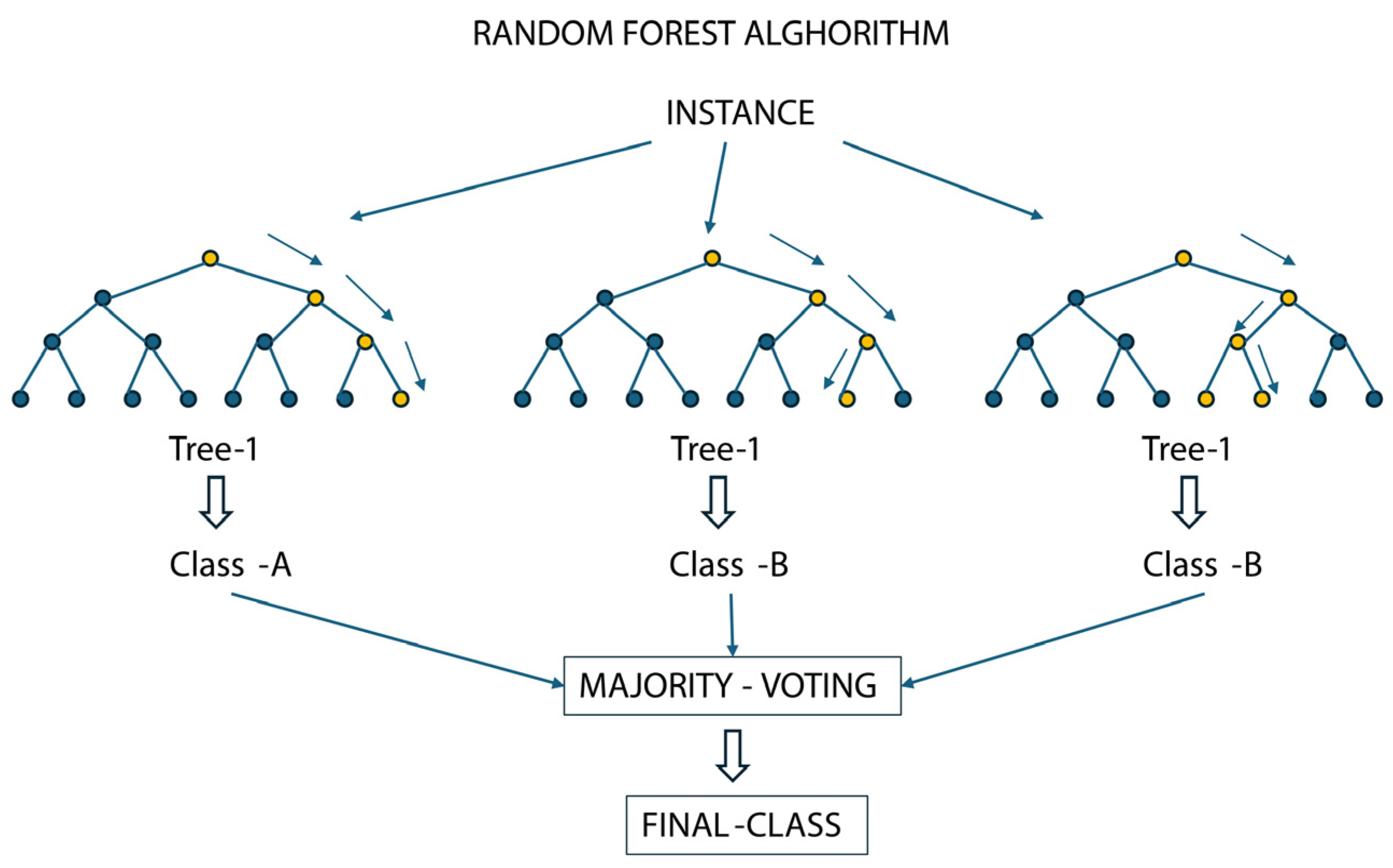
RF [43,81] consists of different Decision Trees [82] that operate together as an ensemble (Figure 3). The concept of RF is that many uncorrelated trees, operating as the voting population, will outperform any of the individual trees. Indeed, one of the most important aspects of RF is the uncorrelation between trees. While some trees may be wrong, many others in the class prediction are correct. So, a set of trees can produce more accurate results due to the uncorrelatedness of the trees. Another advantage of RF is the simplicity of extraction of the most important features in a prediction. The relative importance of each feature’s ability to influence prediction can be calculated by measuring how much the tree node reduces impurity to all trees in the forest using that feature, as described in Equation (2):
N k i = w k C k w l e f t k C l e f t k w r i g h t k C r i g h t k
where w k is the weighted number of samples in node k as a fraction of the total weighted number of samples, C k is the impurity in node k , and l e f t k and r i g h t k are its respective children’s nodes. To obtain a complete map of which features are important for the final classification, we compute a score for each feature after the training phase (Equation (3)) and normalise the results so that the sum of all importances equals 1.
F I i = k : n o d e k s p l i t s o n f e a t u r e i N k i j a l l n o d e s N j i
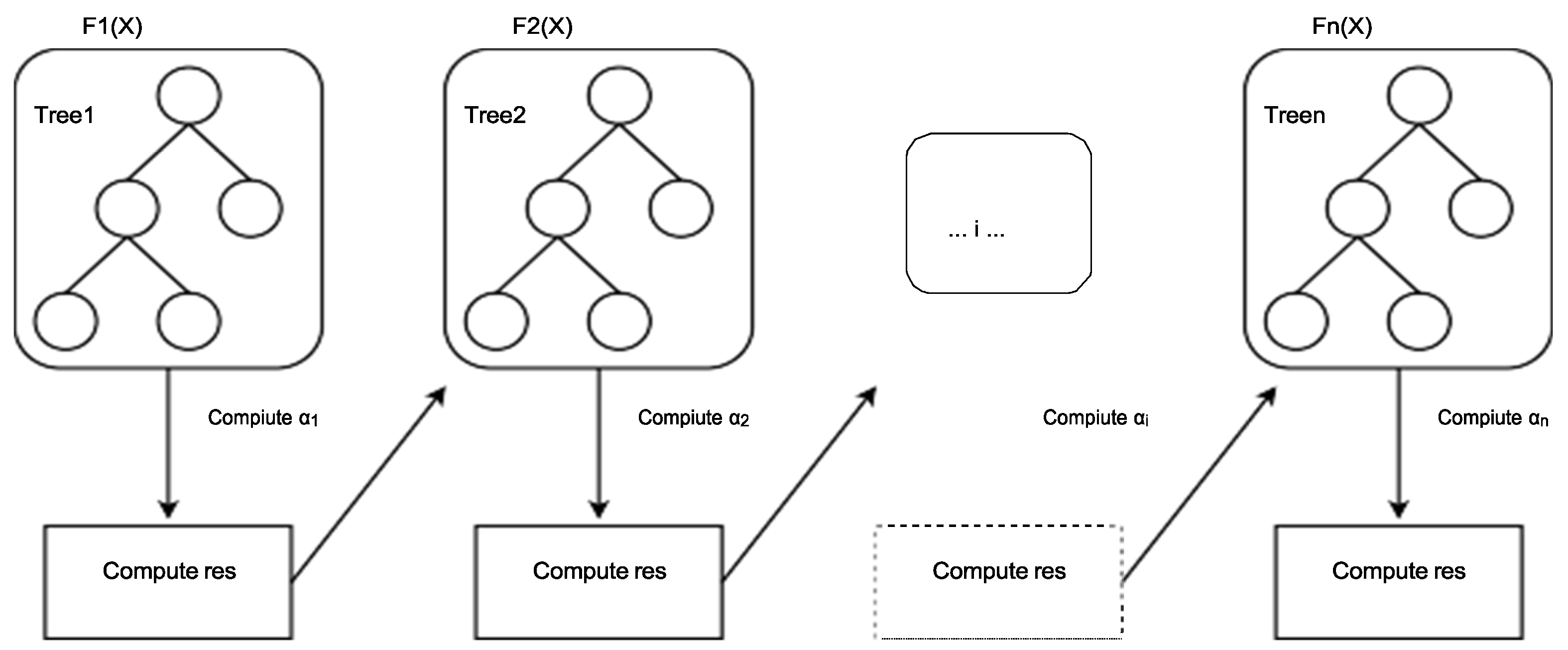
XGB [42,83] is built on the concept of Gradient Boosting [84] (Figure 4). Each weak learner component of the whole ensemble (i.e., Decision Tree) maps input data to one of its leaves that contains a class. The XGB algorithm minimises a regularised loss function (difference between the predicted and target outputs). XGB is trained iteratively. Trees are individually added to the ensemble and adjusted to correct prediction errors from previous models. XGB uses a gradient descent algorithm [85] to minimise loss when adding new weaker models.
In Equation (4), we can see the result of XGB as the sum of previous output K n 1 X and the result of function h n trained to predict result r m 1 multiplied by the regularisation term α n . The r i term represents the output of the ith weaker learner. In Equation (5), we can see how to compute the regularisation term ( α i ), where O i and K i 1 X i are the target output and prediction of the model, respectively. Equation (6) is the differentiable loss function. As for RF, it is possible to obtain the feature importance from XGB by measuring how much the tree nodes using a feature reduce the impurity across all trees in the model.
K n X = K n 1 X + α n h n X , r m 1
a r g m i n α = i = 1 n L O i , K i 1 X i + α h i X i , r i 1
L o s s O , K X
The simulations were performed, splitting the dataset into 80% for training and 20% for the test [86]. Oversampling was used to avoid inconsistency due to the difference between the size of the two addressed classes [87], and a grid search approach was used for the tuning of hyperparameters [88] owing to the moderate size of the dataset.

2.6. Slope Stability Numerical Modeling

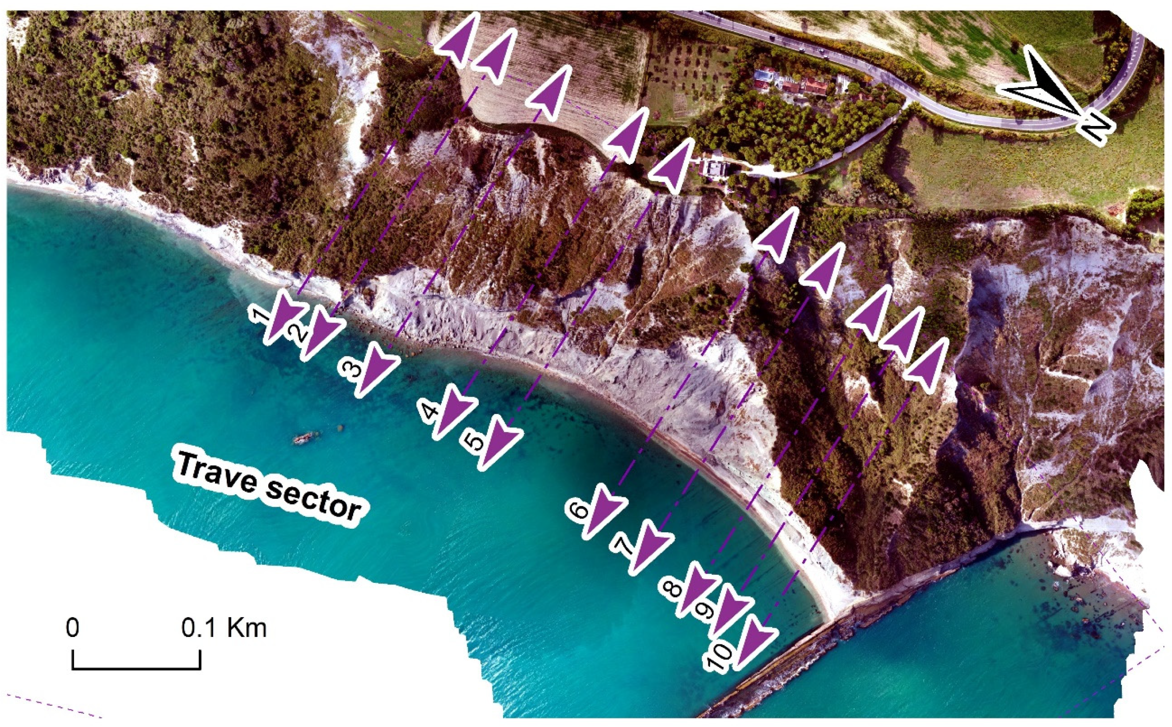
The stability of the Trave sector, i.e., the area most affected by erosion processes in the time span 1978–2022 and showing the highest elevation, has been investigated using the 2D Limit Equilibrium Method (LEM). Ten topographic sections were extracted (Figure 5) from Lidar data provided by Regione Marche in 2012 [48], and the Factor of Safety (FS) was calculated for each of them.
In particular, the slope stability conditions were investigated using the Morgenstern–Price method, implemented in the Slide2 code (accessed on 14 July 2024, https://www.rocscience.com/) on 2012 sections, in order to calculate their F.S. [89].
The input parameters were derived from the field surveys (UCS and GSI classification for complex formation [58]). The Geological Strength Index (GSI) provides a method of relating geological field observations to the quality of the rock mass. This classification is based on the density of jointing and the amount of weathering/alteration observed in the rock mass. As part of the Hoek–Brown Failure Criterion, GSI can be extended to determine the strength and material characteristics of in situ rock masses. The analyses were run, assigning the Hoek–Brown (H-B) failure criterion [90] to the slope materials. GSI was estimated in situ for the different formations, and ranges between 50 and 20. The mi (material constant for the intact rock) and γ (specific weight) parameters were derived from literature [91]. D is a factor which depends upon the degree of disturbance to which the rock mass has been subjected by blast damage and stress relaxation. It varies from 0 for undisturbed in situ rock masses to 1 for very disturbed rock masses. Values of D different from zero indicate disturbed tectonic conditions. Representative values of the materials used in the analyses are listed in Table 2, grouped on the basis of transects values. The models were developed based on the dry conditions of the slopes.

3. Results

3.1. Fieldwork

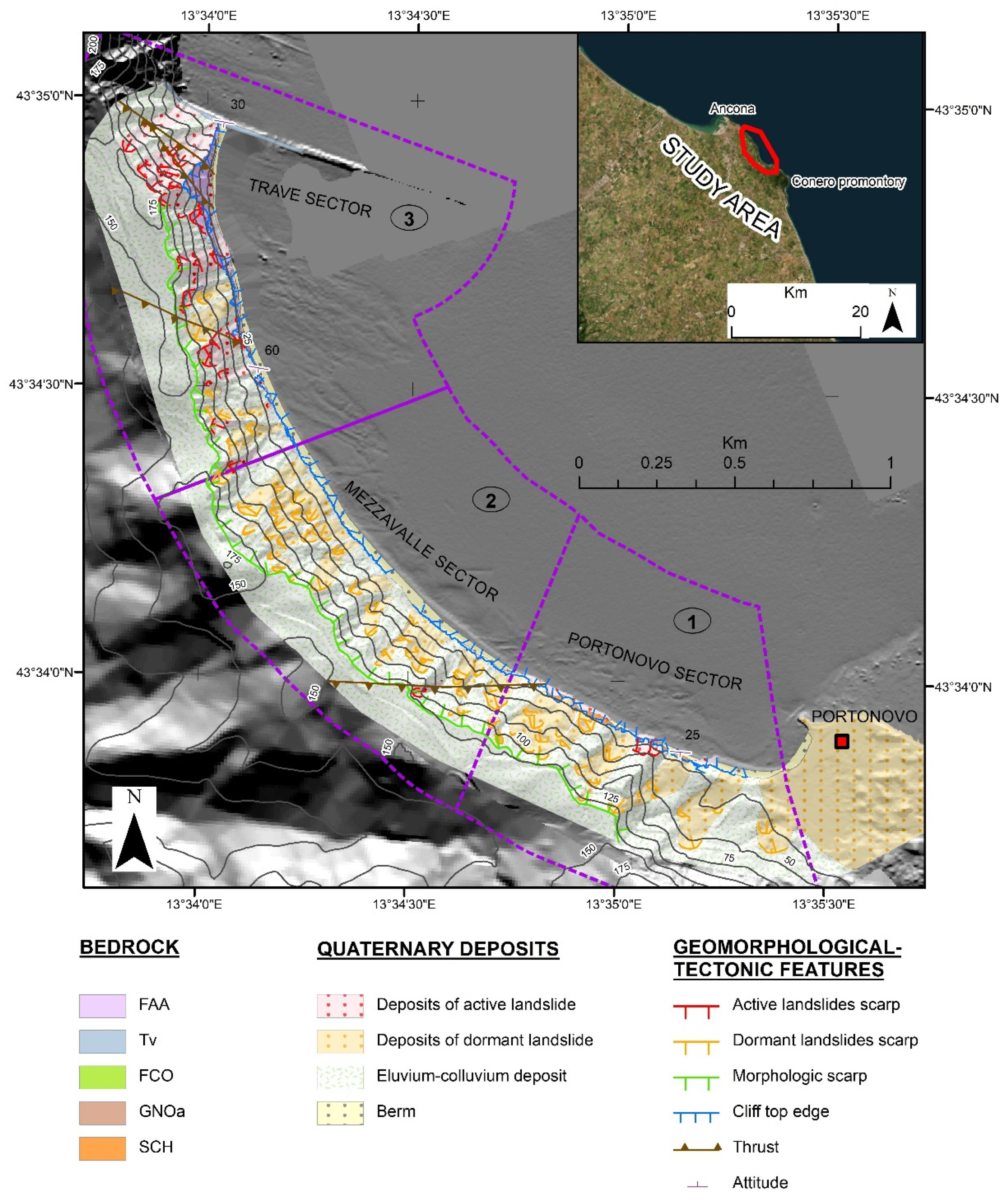
A revised geological/geomorphological setting of the study area was generated based on the field survey findings (Figure 6). The Portonovo sector is characterised by the Schlier Fm., mostly covered by landslides deposits. The height of the cliffs in this sector span from a few meters to a maximum of 30–40 m. Here, the cliff top retreat is mainly determined by landslides in the upper portion of the slope, with vertical or sub-vertical slope faces corresponding to the crown of the landslides (Figure 7a).
The Mezzavalle sector is principally composed by landslide deposit (Figure 7b), with the bedrock outcropping only in the upper and steepest part of the slopes (representing landslides scars). The Trave sector presents the higher numbers of active landslides of different types (rock falls, block toppling, earth flow and complex landslides). An important feature that characterises this sector is the high fracturing degree of the rock mass (Figure 7c), especially in proximity of the thrusts outcropping in this sector.
The UCS values, gathered through pocket penetrometer and Schmidt hammer, are reported in Table 3. Because weak rock masses consist of alternating layers of marls and layers of calcareous marls, an average UCS value was computed across various levels in order to obtain a single representative value for each site. In the areas characterised by landslide deposits or soils, a GSI of 0 was set for the ML analysis.

3.2. Cliff Top Retreat Analysis

The maximum Root Mean Square Error (RMSE) for the digitalisation of the cliff top and the shoreline was calculated. An RMSE of 3.89 m was recorded for cliff top digitalisation using the 1978 orthophoto, while shoreline digitalisation in the 2022 orthophoto yielded an RMSE of 1.65 m. The georeferencing error for the UAV orthophotos using GCPs resulted in a horizontal uncertainty of 5 cm. The horizontal uncertainty between the UAV 2022 orthophoto and the 1978 orthophoto was computed as described in Bloom et al. 2023 [71], and is reported in Figure 8.
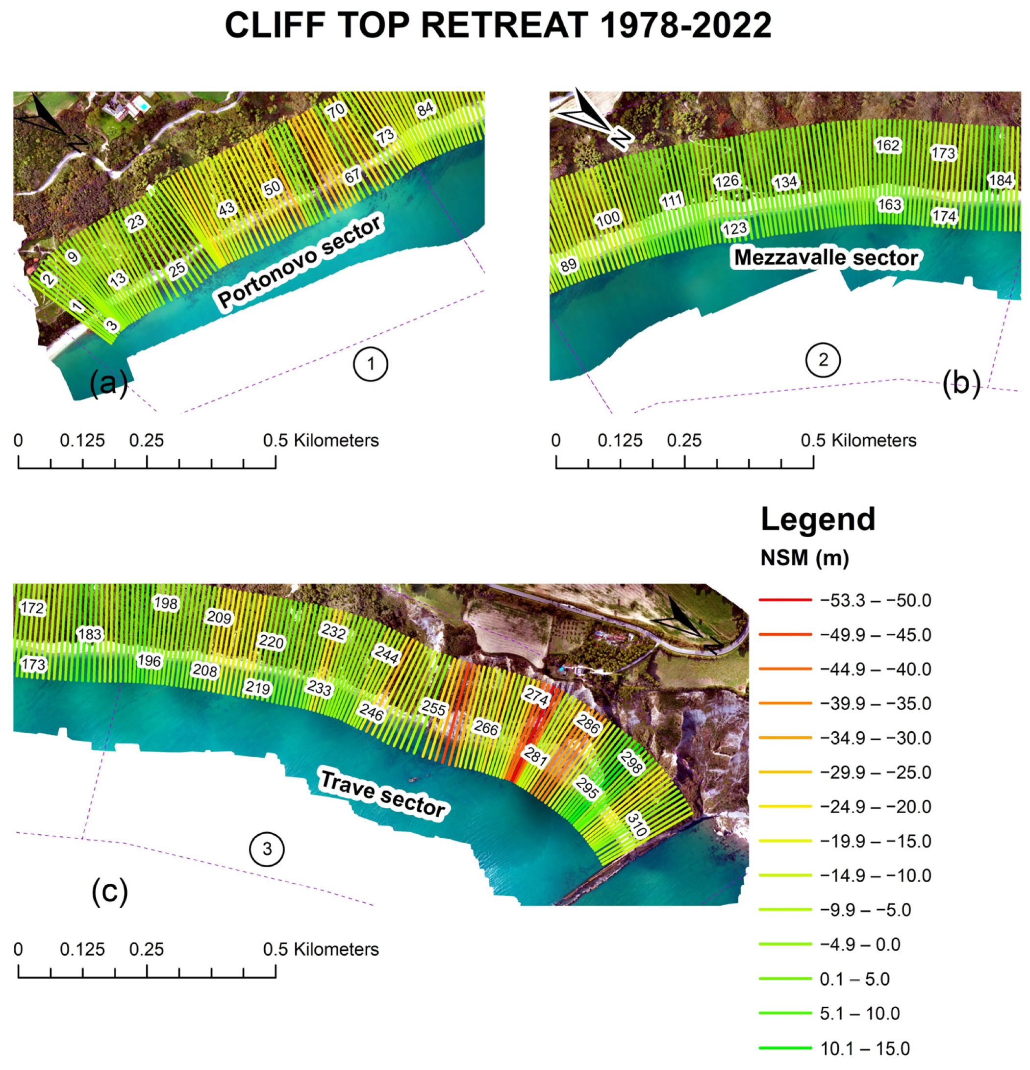
The cliff top erosion in the whole period of 1978–2022 was considered in this analysis. The Trave sector is the portion with the highest mean value of EPR, with peaks of NSM around 50 m; the Portonovo sector shows similar behaviour, but with maximum NSM between 30 and 40 m; while the Mezzavalle sector shows a marginally EPR negative value and insignificant NSM values (Table 4). Moreover, focusing on a/the specific area within each sector, values of almost −0.6 m/yr and −1.2 m/yr of EPR are reached between transects 61–66 and 251–288 in the Portonovo and Trave sectors, respectively (Figure 9). The ECI computed for this time span is 0.09 m.

3.3. Machine Learning

The parameters shown in Table 1 were extracted for each transect, yielding a dataset with 310 lines (corresponding to the number of transects) and 13 data columns, denoting the 13 extracted or derived parameters for each transect (Supplementary Materials). These data were processed through two ML algorithms, RF and XGB, as described in the methodology section.
Each algorithm gave two different outputs: a confusion matrix and a table with feature importance.
RF analysis gave a test score of 0.95 on test data, and a confusion matrix showing only four false predictions (Figure 10, 3b). The feature significance graph (Figure 10, 3a) revealed that “Cliff height” is the most important parameter for class prediction, with a relative relevance twice that of the other drivers.
The XGB algorithm reported a test score of 0.95 on test data. The confusion matrix (Figure 10, 3d) for XGB revealed four erroneous predictions, and the feature importance graph (Figure 10, 3c) revealed the same order gathered from the RF algorithm. Also, in this case, “Cliff Height” was shown to be the most relevant characteristic in class recognition.

3.4. Slope Stability

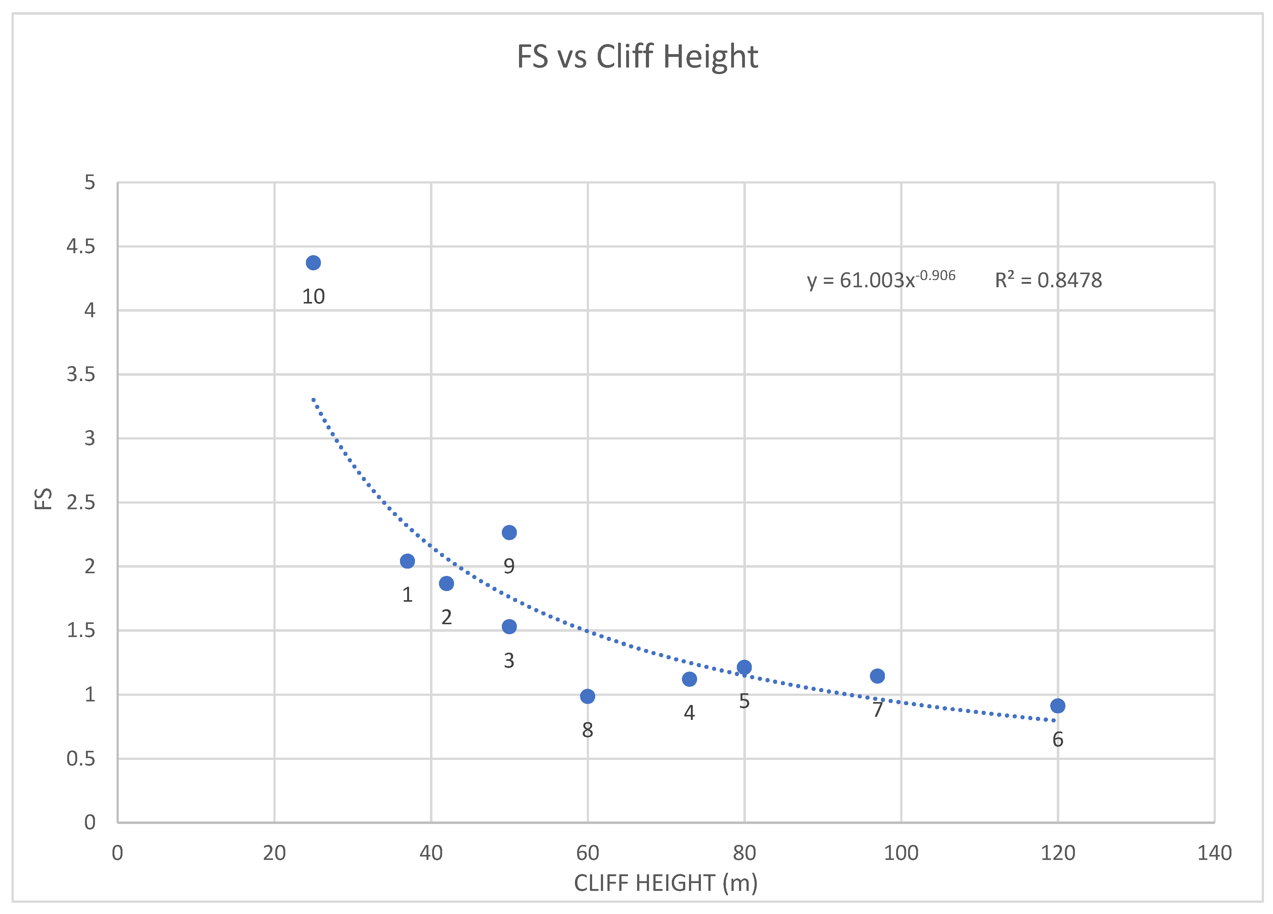
Numerical modeling outputs are reported for convenience in Table 5, summarising the FS and cliff height values obtained. Values of FS below 1 are present in Sections 6 and 8, and the range of values obtained is from 4.37 to 0.91. Notably, these are indicative of the greater and lower cliff heights, respectively.
The graph in Figure 11 highlights the correlation between FS and cliff height (R2 = 0.84), with FS values decreasing with slope elevation. Section 6, with a FS of 0.91, crosses the slope between transects 280–290, where values of retreat above 40 m in the period 1978–2022 were computed.

4. Discussion

This research aimed to show a multidisciplinary approach to the study of coastal cliff retreat based on the use of DSAS, ML analysis and numerical modeling. The cliff top retreat analysis closely corroborates the results gathered by previous research [48]. Notably, this analysis confirms that the Trave sector remains the most precarious and unstable segment of the coastline, manifesting higher NSM in certain transects when compared to the Portonovo sector. The mean EPR shows similar patterns for these latter two sectors. The Mezzavalle sector continues to exhibit a lower evolutional rate when compared with the other two sectors. However, it is necessary to emphasise that further research, employing enhanced spatial resolution techniques, is required to discern the seasonal variations in the evolution of these cliffs, predominantly constituted by landslide deposits. The coastal cliff retreat on weak rocks calculated in other works showed an average retreat similar to the calculations in our study area, with the exception of the Trave sector, where the erosion rate is three times higher than the average in GlobR2C2 [21,54,74]. Still, in the Adriatic sea, mean EPR values similar to the ones estimated in our research were found in two areas of the Puglia Region (0.08 m/yr and 0.12 m/yr) [27,92], two areas of the Abruzzo Region (0.15 m/yr and 1 m/yr) [93] and in the Marche Region (0.16 m/yr) [94].
Numerous works have attempted to comprehend the drivers behind cliff retreat [5,54,64,72,95,96,97,98,99]. Thus, in this study, we presented a new and innovative approach to investigating cliff top erosion. Only a few similar approaches have been attempted: Dickson and Perry 2016 [36] focused on different ML techniques, such as classification and regression trees (CART), maximum entropy models (MAXENT) and boosted regression trees (BRT), and applied them to wide scales to identify more dangerous areas. He et al. 2021 [37] used the RF algorithm and support vector machine (SVM), multilayer perceptron (MLP) and deep learning neural network (DLNN) models to evaluate the role of the orientation of discontinuities in landslide processes. By contrast, in the current work, we focused on analysing a site specific case study, taking into account a large number of drivers and proposing a specific methodology to assess the importance of the different factors in the erosional process. ML applications similar to the ones presented in this research have previously demonstrated their efficacy in various scientific domains [100,101,102,103,104,105]. The robustness of results and the absence of overfitting in relation to the training dataset are ensured by the high test scores achieved through ML analysis, coupled with the utilisation of grid search, oversampling techniques and bagging.
In the context of the parameters chosen for the ML algorithms, it is important to acknowledge that the compilation of driving factors presented here does not represent an exhaustive inventory encompassing all imaginable elements influencing cliff failure. The selection of these factors has been guided by comprehensive reviews of prior research [5,35,72,106], on-site investigations, and the practical constraints inherent in fieldwork. It is worth noting that future research endeavors may consider expanding the analysis to encompass marine drivers. A study of nearshore bathymetry, followed by numerical wave propagation modeling to derive significant wave height values at the cliff base, could be performed [26,74,107]. Furthermore, the ML code employed in this research has been made available on GitHub (accessed on 14 July 2024, https://github.com/micheleFraccaroli/Machine-Learning-for-Coastal-Retreat). This will facilitate the potential application of our methodology by other researchers to different sites, permitting the assessment of its consistency and the incorporation of additional parameters in other geological/marine contexts.
Furthermore, RF and XGB algorithms, if compared to neural networks, have the benefit of not requiring a large amount of data to achieve excellent results. Furthermore, they have an intrinsic ‘explainability’. Both RF and XGB are ‘transparent’ algorithms, meaning they are explainable by design. What we needed in our work was not the prediction from the Machine Learning algorithm itself, but the associated explanation. In other words, we were interested in knowing which features were the most important in ‘explaining’ a given prediction.
The most significant result from both Mean Decrease in Impurity (MDI) studies emphasises the importance of cliff height in cliff top erosion. This connection has previously been documented in the literature [36,73,108,109,110].
To further investigate the retreat mechanism and the role of cliff height, numerical modeling of the slopes was undertaken. Particularly, ten sections were extracted in the Trave sector, where the greatest height and NSM were recorded. In this context, the LEM approach, considering circular surfaces of slip, was judged appropriate, as the slope can be approximated as an isotropic continua with respect to its lithological properties [44]. The simulation results align with the ML findings, confirming the link between FS and cliff height. However, it is remarkable that in many sections, the calculated Safety Factor (SRF) remains near 1 or below. This agrees with the frequent, almost daily, activity observed in these slopes, characterised by isolated falls or toppling events. Any perturbations, either resulting from changes in pore pressure, seismic activity, or clay shrinkage, can trigger landslide events. Previous research on rocky coastlines has undertaken numerical slope modeling, taking into account the evolving notches at various locations on the cliffs (e.g., base and middle, particularly in cases of pronounced lithological contrasts) to elucidate the stress–strain response within the changed topographic configuration [27,111]. To complete these objectives, further research such as laboratory testing, borehole explorations, and more sophisticated softwares such as Finite Element Methods (FEMs) are required. The present study did not pursue this line of investigation; instead, it focused on assessing the correlation between cliff height and retrieved FS, just to potentially validate the ML finding. Furthermore, although geological structural information is embedded in the parameters of GSI and UCS, it is essential to consider that these parameters were gathered at the cliff base because of logistical difficulties (e.g., operator safety) in accessing the cliff top.
This study serves as a site specific analysis employing an ML approach to discern the significance of diverse parameters in cliff top retreat. If successfully replicated in other locations, this methodology can potentially inform engineering design solutions. It offers valuable insights into which specific factors, among the multitude of influencing variables, favor targeted interventions to mitigate instability.

5. Conclusions

The main achievements of this research can be summarised as follows:
  • Cliff top retreat calculations spanning the period from 1978 to 2022 reaffirm the findings of previous research [48], indicating notably higher values of NSM in the Trave sector.
  • The Mean Decrease in Impurity (MDI) analysis, conducted utilising Random Forest (RF) and XGBoost (XGB) ML algorithms, identified cliff height as the most significant parameter for cliff top erosion.
  • Limit Equilibrium Method (LEM) modeling confirms the correlation between FS and cliff height.
Subsequent investigations will require a thorough analysis of marine parameters (e.g., significant wave height, high resolution bathymetry). These could be included in various additional cases studies to evaluate the efficacy of the algorithms.
A GitHub repository containing the machine learning (ML) code employed for this analysis has been made available to facilitate the reproducibility of this study in different locations (accessed on 14 July 2024, https://github.com/micheleFraccaroli/Machine-Learning-for-Coastal-Retreat).
If successfully applied to different case studies and geological/marine settings, this methodology could have the potential of improving decision making for coastal risk management.

Supplementary Materials

The following supporting information can be downloaded at: https://www.mdpi.com/article/10.3390/rs16142604/s1, Table S1: Input data for machine learning analysis.

Author Contributions

Conceptualisation: N.F.; methodology N.F., M.F. (Michele Fraccaroli), M.F. (Mirko Francioni), S.F., A.B., P.C. and M.G.; validation: N.F., M.F. (Michele Fraccaroli), M.F. (Mirko Francioni), S.F., A.B., P.C. and M.G.; formal analysis: N.F., M.F. (Mirko Francioni), S.F., A.B., M.G. and P.C.; investigation: N.F., M.F. (Mirko Francioni) and A.B.; resources: M.G. and M.F. (Mirko Francioni); data curation: N.F., M.F. (Michele Fraccaroli) and M.F. (Mirko Francioni); writing—original draft preparation: N.F.; writing—review and editing: N.F., M.F. (Michele Fraccaroli), M.F. (Mirko Francioni), S.F., A.B., P.C. and M.G.; project administration: M.G. and M.F. (Mirko Francioni); funding acquisition: M.G. and M.F. (Mirko Francioni). All authors have read and agreed to the published version of the manuscript.

Funding

Founded by Interreg Italy-Croatia Programme 2021-27, 1st call for proposals, standard project proposal. Project: RESONANCE (impRoving landslidE riSk preventiOn aNd mAnagement iN Coastal arEas), P.I.: Mirko Francioni, University of Urbino, Carlo Bo- and by EMAS PhD funds.

Data Availability Statement

The data presented in this study are available on request from the corresponding author.

Acknowledgments

We want to express our gratitude to the people that have supported the field work and shared useful advice, in particular Alessia Sciati and Enrico Duo. Also, we would like to express our thanks to Il Parco del Conero and Regione Marche (in particular to Stefano Parlani), for sharing the data.

Conflicts of Interest

The authors declare no conflicts of interest.

References

  1. Martínez, M.L.; Intralawan, A.; Vázquez, G.; Pérez-Maqueo, O.; Sutton, P.; Landgrave, R. The Coasts of Our World: Ecological, Economic and Social Importance. Ecol. Econ. 2007, 63, 254–272. [Google Scholar] [CrossRef]
  2. Young, A.P.; Carilli, J.E. Global Distribution of Coastal Cliffs. Earth Surf. Process. Landforms 2019, 44, 1309–1316. [Google Scholar] [CrossRef]
  3. Naylor, L.A.; Stephenson, W.J.; Trenhaile, A.S. Rock Coast Geomorphology: Recent Advances and Future Research Directions. Geomorphology 2010, 114, 3–11. [Google Scholar] [CrossRef]
  4. Kennedy, D.M.; Paulik, R.; Dickson, M.E. Subaerial Weathering versus Wave Processes in Shore Platform Development: Reappraising the Old Hat Island Evidence. Earth Surf. Process. Landforms 2011, 36, 686–694. [Google Scholar] [CrossRef]
  5. Sunamura, T. Rocky Coast Processes: With Special Reference to the Recession of Soft Rock Cliffs. Proc. Japan Acad. Ser. B Phys. Biol. Sci. 2015, 91, 481–500. [Google Scholar] [CrossRef] [PubMed]
  6. Poate, T.; Masselink, G.; Austin, M.J.; Dickson, M.; McCall, R. The Role of Bed Roughness in Wave Transformation Across Sloping Rock Shore Platforms. J. Geophys. Res. Earth Surf. 2018, 123, 91–123. [Google Scholar] [CrossRef]
  7. Moses, C.; Robinson, D. Chalk Coast Dynamics: Implications for Understanding Rock Coast Evolution. Earth-Sci. Rev. 2011, 109, 63–73. [Google Scholar] [CrossRef]
  8. Kennedy, D.M.; Milkins, J. The Formation of Beaches on Shore Platforms in Microtidal Environments. Earth Surf. Process. Landforms 2015, 40, 34–46. [Google Scholar] [CrossRef]
  9. Sunamura, T. The Elevation of Shore Platforms: A Laboratory Approach to the Unsolved Problem. J. Geol. 1991, 99, 761–766. [Google Scholar] [CrossRef]
  10. Robinson, A.H.W. Erosion and Accretion along Part of the Suffolk Coast of East Anglia, England. Mar. Geol. 1980, 37, 133–146. [Google Scholar] [CrossRef]
  11. Troiani, F.; Martino, S.; Marmoni, G.M.; Menichetti, M.; Torre, D.; Iacobucci, G.; Piacentini, D. Integrated Field Surveying and Land Surface Quantitative Analysis to Assess Landslide Proneness in the Conero Promontory Rocky Coast (Italy). Appl. Sci. 2020, 14, 4793. [Google Scholar] [CrossRef]
  12. Naylor, L.A.; Stephenson, W.J. On the Role of Discontinuities in Mediating Shore Platform Erosion. Geomorphology 2010, 114, 89–100. [Google Scholar] [CrossRef]
  13. Donati, D.; Stead, D.; Lato, M.; Gaib, S. Spatio-Temporal Characterization of Slope Damage: Insights from the Ten Mile Slide, British Columbia, Canada. Landslides 2020, 17, 1037–1049. [Google Scholar] [CrossRef]
  14. Marmoni, G.M.; Martino, S.; Censi, M.; Menichetti, M.; Piacentini, D.; Scarascia Mugnozza, G.; Torre, D.; Troiani, F. Transition from Rock Mass Creep to Progressive Failure for Rockslide Initiation at Mt. Conero (Italy). Geomorphology 2023, 437, 108750. [Google Scholar] [CrossRef]
  15. Rosser, N.J.; Brain, M.J.; Petley, D.N.; Lim, M.; Norman, E.C. Coastline Retreat via Progressive Failure of Rocky Coastal Cliffs. Geology 2013, 41, 939–942. [Google Scholar] [CrossRef]
  16. Caputo, T.; Marino, E.; Matano, F.; Somma, R.; Troise, C.; De Natale, G. Terrestrial Laser Scanning (TLS) Data for the Analysis of Coastal Tuff Cliff Retreat: Application to Coroglio Cliff, Naples, Italy. Ann. Geophys. Geophys. 2018, 61, SE110. [Google Scholar] [CrossRef]
  17. Esposito, G.; Salvini, R.; Matano, F.; Sacchi, M.; Danzi, M.; Somma, R.; Troise, C. Multitemporal Monitoring of a Coastal Landslide through SfM-Derived Point Cloud Comparison. Photogramm. Rec. 2017, 32, 459–479. [Google Scholar] [CrossRef]
  18. Matano, F.; Pignalosa, A.; Marino, E.; Esposito, G.; Caccavale, M.; Caputo, T.; Sacchi, M.; Somma, R.; Troise, C.; De Natale, G. Laser Scanning Application for Geostructural Analysis of Tuffaceous Coastal Cliffs: The Case of Punta Epitaffio, Pozzuoli Bay, Italy. Eur. J. Remote Sens. 2015, 48, 615–637. [Google Scholar] [CrossRef]
  19. Loiotine, L.; Andriani, G.F.; Jaboyedoff, M.; Parise, M.; Derron, M.H. Comparison of Remote Sensing Techniques for Geostructural Analysis and Cliff Monitoring in Coastal Areas of High Tourist Attraction: The Case Study of Polignano a Mare (Southern Italy). Remote Sens. 2021, 13, 5045. [Google Scholar] [CrossRef]
  20. Francioni, M.; Coggan, J.; Eyre, M.; Stead, D. A Combined Field/Remote Sensing Approach for Characterizing Landslide Risk in Coastal Areas. Int. J. Appl. Earth Obs. Geoinf. 2018, 67, 79–95. [Google Scholar] [CrossRef]
  21. Gómez-Pazo, A.; Pérez-Alberti, A.; Trenhaile, A. Tracking the Behavior of Rocky Coastal Cliffs in Northwestern Spain. Environ. Earth Sci. 2021, 80, 1–18. [Google Scholar] [CrossRef]
  22. Prémaillon, M.; Dewez, T.J.B.; Regard, V.; Rosser, N.J.; Carretier, S.; Guillen, L. Conceptual Model of Fracture-Limited Sea Cliff Erosion: Erosion of the Seaward Tilted Flyschs of Socoa, Basque Country, France. Earth Surf. Process. Landforms 2021, 46, 2690–2709. [Google Scholar] [CrossRef]
  23. Young, A.P.; Guza, R.T.; Matsumoto, H.; Merrifield, M.A.; O’Reilly, W.C.; Swirad, Z.M. Three Years of Weekly Observations of Coastal Cliff Erosion by Waves and Rainfall. Geomorphology 2021, 375, 107545. [Google Scholar] [CrossRef]
  24. Piacentini, D.; Troiani, F.; Torre, D.; Menichetti, M. Land-Surface Quantitative Analysis to Investigate the Spatial Distribution of Gravitational Landforms along Rocky Coasts. Remote Sens. 2021, 13, 5012. [Google Scholar] [CrossRef]
  25. Jaud, M.; Letortu, P.; Théry, C.; Grandjean, P.; Costa, S.; Maquaire, O.; Davidson, R.; Le Dantec, N. UAV Survey of a Coastal Cliff Face—Selection of the Best Imaging Angle. Measurement 2019, 139, 10–20. [Google Scholar] [CrossRef]
  26. Bergillos, R.J.; Rodriguez-Delgado, C.; Medina, L.; Fernandez-Ruiz, J.; Rodriguez-Ortiz, J.M.; Iglesias, G. A Combined Approach to Cliff Characterization: Cliff Stability Index. Mar. Geol. 2022, 444, 106706. [Google Scholar] [CrossRef]
  27. Lollino, P.; Pagliarulo, R.; Trizzino, R.; Santaloia, F.; Pisano, L.; Zumpano, V.; Perrotti, M.; Fazio, N.L. Multi-Scale Approach to Analyse the Evolution of Soft Rock Coastal Cliffs and Role of Controlling Factors: A Case Study in South-Eastern Italy. Geomat. Nat. Hazards Risk 2021, 12, 1058–1081. [Google Scholar] [CrossRef]
  28. Earlie, C.S.; Masselink, G.; Russell, P.E.; Shail, R.K. Application of Airborne LiDAR to Investigate Rates of Recession in Rocky Coast Environments. J. Coast. Conserv. 2015, 19, 831–845. [Google Scholar] [CrossRef]
  29. Torre, D.; Galve, J.P.; Reyes-Carmona, C.; Alfonso-Jorde, D.; Ballesteros, D.; Menichetti, M.; Piacentini, D.; Troiani, F.; Azañón, J.M. Geomorphological Assessment as Basic Complement of InSAR Analysis for Landslide Processes Understanding. Landslides 2024, 21, 1273–1292. [Google Scholar] [CrossRef]
  30. Mantovani, M.; Devoto, S.; Forte, E.; Mocnik, A.; Pasuto, A.; Piacentini, D.; Soldati, M. A Multidisciplinary Approach for Rock Spreading and Block Sliding Investigation in the North-Western Coast of Malta. Landslides 2013, 10, 611–622. [Google Scholar] [CrossRef]
  31. Di Luccio, D.; Aucelli, P.P.C.; Di Paola, G.; Pennetta, M.; Berti, M.; Budillon, G.; Florio, A.; Benassai, G. An Integrated Approach for Coastal Cliff Susceptibility: The Case Study of Procida Island (Southern Italy). Sci. Total Environ. 2023, 855, 158759. [Google Scholar] [CrossRef] [PubMed]
  32. Del Río, L.; Gracia, F.J. Erosion Risk Assessment of Active Coastal Cliffs in Temperate Environments. Geomorphology 2009, 112, 82–95. [Google Scholar] [CrossRef]
  33. Anfuso, G.; Gracia, F.J.; Battocletti, G. Determination of Cliffed Coastline Sensitivity and Associated Risk for Human Structures: A Methodological Approach. J. Coast. Res. 2013, 29, 1292–1296. [Google Scholar] [CrossRef]
  34. Tursi, M.F.; Anfuso, G.; Matano, F.; Mattei, G.; Aucelli, P.P.C. A Methodological Tool to Assess Erosion Susceptibility of High Coastal Sectors: Case Studies from Campania Region (Southern Italy). Water 2023, 15, 121. [Google Scholar] [CrossRef]
  35. Hapke, C.; Plant, N. Predicting Coastal Cliff Erosion Using a Bayesian Probabilistic Model. Mar. Geol. 2010, 278, 140–149. [Google Scholar] [CrossRef]
  36. Dickson, M.E.; Perry, G.L.W. Identifying the Controls on Coastal Cliff Landslides Using Machine-Learning Approaches. Environ. Model. Softw. 2016, 76, 117–127. [Google Scholar] [CrossRef]
  37. He, L.; Coggan, J.; Francioni, M.; Eyre, M. Maximizing Impacts of Remote Sensing Surveys in Slope Stability—A Novel Method to Incorporate Discontinuities into Machine Learning Landslide Prediction. ISPRS Int. J. Geo-Inf. 2021, 10, 232. [Google Scholar] [CrossRef]
  38. Himmelstoss, E.A.; Henderson, R.E.; Kratzmann, M.G.; Farris, A.S. Digital Shoreline Analysis System (DSAS) Version 5.0 User Guide; Open-File Report 2018-1179; U.S. Geological Survey: Woods Hole, MA, USA, 2018. [Google Scholar]
  39. Apostolopoulos, D.N.; Nikolakopoulos, K.G. Identifying Sandy Sites under Erosion Regime along the Prefecture of Achaia, Using Remote Sensing Techniques. J. Appl. Remote Sens. 2023, 17, 22206. [Google Scholar] [CrossRef]
  40. Dey, M.; Jena, B.K. A Shoreline Change Detection (2012–2021) and Forecasting Using Digital Shoreline Analysis System (DSAS) Tool: A Case Study of Dahej Coast, Gulf of Khambhat, Gujarat, India. Indones. J. Geogr. 2021, 53, 295. [Google Scholar] [CrossRef]
  41. Chrisben Sam, S.; Gurugnanam, B. Coastal Transgression and Regression from 1980 to 2020 and Shoreline Forecasting for 2030 and 2040, Using DSAS along the Southern Coastal Tip of Peninsular India. Geod. Geodyn. 2022, 13, 585–594. [Google Scholar] [CrossRef]
  42. Chen, T.; Guestrin, C. XGBoost: A Scalable Tree Boosting System. In Proceedings of the 22nd ACM SIGKDD International Conference on Knowledge Discovery and Data Mining, San Francisco, CA, USA, 13–17 August 2016; pp. 785–794. [Google Scholar] [CrossRef]
  43. Breiman, L. Random Forests. Mach. Learn. 2001, 45, 5–32. [Google Scholar] [CrossRef]
  44. Stead, D.; Coggan, J. Numerical Modeling of Rock-Slope Instability. In Landslides: Types, Mechanisms and Modeling; Stead, D., Clague, J.J., Eds.; Cambridge University Press: Cambridge, UK, 2012; pp. 144–158. ISBN 9781107002067. [Google Scholar]
  45. Cello, G.; Coppola, L. Modalità e Stili Deformativi Nell’area Anconetana. Stud. Geol. Camerti 1989, XI, 37–48. [Google Scholar]
  46. Coltorti, M.; Sarti, M. Note Illustrative Della Carta Geologica d’Italia Alla Scala 1:50.000 “Foglio 293—Osimo”. Progetto CARG: ISPRA, Servizio Geologico d’Italia. 2011. Available online: https://www.isprambiente.gov.it/Media/carg/293_OSIMO/Foglio.html (accessed on 14 July 2024).
  47. Montanari, A.; Mainiero, M.; Coccioni, R.; Pignocchi, G. Catastrophic Landslide of Medieval Portonovo (Ancona, Italy). Geol. Soc. Am. Bull. 2016, 128, 1660–1678. [Google Scholar] [CrossRef]
  48. Fullin, N.; Duo, E.; Fabbri, S.; Francioni, M.; Ghirotti, M.; Ciavola, P. Quantitative Characterization of Coastal Cliff Retreat and Landslide Processes at Portonovo—Trave Cliffs (Conero, Ancona, Italy) Using Multi-Source Remote Sensing Data. Remote Sens. 2023, 15, 4120. [Google Scholar] [CrossRef]
  49. Hungr, O.; Leroueil, S.; Picarelli, L. The Varnes Classification of Landslide Types, an Update. Landslides 2014, 11, 167–194. [Google Scholar] [CrossRef]
  50. Cruden, D.M.; Varnes, D.J. Landslide Types and Processes, Transportation Research Board, U.S. National Academy of Sciences, Special Report. Spec. Rep.-Natl. Res. Counc. Transp. Res. Board 1996, 247, 36–57. [Google Scholar]
  51. Bisci, C.; Cantalamessa, G.; de Marco, R.; Spagnoli, F.; Tramontana, M. Caratteri Oceanografici Dell’Adriatico Centro-Settentrionale e Della Costa Marchigiana. Stud. Costieri 2021, 30, 7–12. [Google Scholar]
  52. Acciarri, A.; Bisci, C.; Cantalamessa, G.; Cappucci, S.; Conti, M.; Di Pancrazio, G.; Spagnoli, F.; Valentini, E. Metrics for Short-Term Coastal Characterization, Protection and Planning Decisions of Sentina Natural Reserve, Italy. Ocean Coast. Manag. 2021, 201, 105472. [Google Scholar] [CrossRef]
  53. Grottoli, E.; Bertoni, D.; Ciavola, P.; Pozzebon, A. Short Term Displacements of Marked Pebbles in the Swash Zone: Focus on Particle Shape and Size. Mar. Geol. 2015, 367, 143–158. [Google Scholar] [CrossRef]
  54. Prémaillon, M.; Regard, V.; Dewez, T.J.B.; Auda, Y. GlobR2C2 (Global Recession Rates of Coastal Cliffs): A Global Relational Database to Investigate Coastal Rocky Cliff Erosion Rate Variations. Earth Surf. Dyn. 2018, 6, 651–668. [Google Scholar] [CrossRef]
  55. Budetta, P.; Galietta, G.; Santo, A. A Methodology for the Study of the Relation between Coastal Cliff Erosion and the Mechanical Strength of Soils and Rock Masses. Eng. Geol. 2000, 56, 243–256. [Google Scholar] [CrossRef]
  56. Barton, N. Suggested Methods for the Quantitative Description of Discontinuities in Rock Masses. Int. J. Rock Mech. Min. Sci. Geomech. Abstr. 1978, 15, 319–368. [Google Scholar]
  57. Hoek, E.; Marinos, P.G.; Marinos, V.P. Characterisation and Engineering Properties of Tectonically Undisturbed but Lithologically Varied Sedimentary Rock Masses. Int. J. Rock Mech. Min. Sci. 2005, 42, 277–285. [Google Scholar] [CrossRef]
  58. Marinos, P.V. New Proposed Gsi Classification Charts for Weak or Complex Rock Masses. Bull. Geol. Soc. Greece 2017, 43, 1248. [Google Scholar] [CrossRef]
  59. Duo, E.; Fabbri, S.; Grottoli, E.; Ciavola, P. Uncertainty of Drone-Derived DEMs and Significance of Detected Morphodynamics in Artificially Scraped Dunes. Remote Sens. 2021, 13, 1823. [Google Scholar] [CrossRef]
  60. Gindraux, S.; Boesch, R.; Farinotti, D. Accuracy Assessment of Digital Surface Models from Unmanned Aerial Vehicles’ Imagery on Glaciers. Remote Sens. 2017, 9, 186. [Google Scholar] [CrossRef]
  61. Brunetta, R.; Duo, E.; Ciavola, P. Evaluating Short-Term Tidal Flat Evolution Through UAV Surveys: A Case Study in the Po Delta (Italy). Remote Sens. 2021, 13, 2322. [Google Scholar] [CrossRef]
  62. Fabbri, S.; Grottoli, E.; Armaroli, C.; Ciavola, P. Using High-Spatial Resolution UAV-Derived Data to Evaluate Vegetation and Geomorphological Changes on a Dune Field Involved in a Restoration Endeavour. Remote Sens. 2021, 13, 1987. [Google Scholar] [CrossRef]
  63. Talavera, L.; Benavente, J.; Del Río, L. UAS Identify and Monitor Unusual Small-Scale Rhythmic Features in the Bay of Cádiz (Spain). Remote Sens. 2021, 13, 1188. [Google Scholar] [CrossRef]
  64. Brooks, S.M.; Spencer, T.; Boreham, S. Deriving Mechanisms and Thresholds for Cliff Retreat in Soft-Rock Cliffs under Changing Climates: Rapidly Retreating Cliffs of the Suffolk Coast, UK. Geomorphology 2012, 153–154, 48–60. [Google Scholar] [CrossRef]
  65. Cenci, L.; Disperati, L.; Sousa, L.P.; Phillips, M.; Alves, F.L. Geomatics for Integrated Coastal Zone Management: Multitemporal Shoreline Analysis and Future Regional Perspective for the Portuguese Central Region. J. Coast. Res. 2013, 65, 1349–1354. [Google Scholar] [CrossRef]
  66. Virdis, S.G.P.; Oggiano, G.; Disperati, L. A Geomatics Approach to Multitemporal Shoreline Analysis in Western Mediterranean: The Case of Platamona-Maritza Beach (Northwest Sardinia, Italy). J. Coast. Res. 2012, 28, 624–640. [Google Scholar] [CrossRef]
  67. Buchanan, D.H.; Naylor, L.A.; Hurst, M.D.; Stephenson, W.J. Erosion of Rocky Shore Platforms by Block Detachment from Layered Stratigraphy. Earth Surf. Process. Landforms 2020, 45, 1028–1037. [Google Scholar] [CrossRef]
  68. Crowell, M.; Leatherman, S.P.; Buckley, M.K. Historical Shoreline Change: Error Analysis and Mapping Accuracy. J. Coast. Res. 1991, 7, 839–852. [Google Scholar]
  69. Fletcher, C.; Rooney, J.; Barbee, M.; Lim, S.; Richmond, B. Mapping Shoreline Change Using Digital Orthophotogrammetry on Maui, Hawaii. J. Coast. Res. 2003, 38, 106–124. [Google Scholar]
  70. Del Río, L.; Gracia, F.J. Error Determination in the Photogrammetric Assessment of Shoreline Changes. Nat. Hazards 2013, 65, 2385–2397. [Google Scholar] [CrossRef]
  71. Bloom, C.K.; Singeisen, C.; Stahl, T.; Howell, A.; Massey, C. Earthquake Contributions to Coastal Cliff Retreat. Earth Surf. Dyn. 2023, 11, 757–778. [Google Scholar] [CrossRef]
  72. Trenhaile, A.S. Cliffs and Rock Coasts; Elsevier Inc.: Amsterdam, The Netherlands, 2012; Volume 3, ISBN 9780080878850. [Google Scholar]
  73. Wolters, G.; Müller, G. Effect of Cliff Shape on Internal Stresses and Rock Slope Stability. J. Coast. Res. 2008, 24, 43–50. [Google Scholar] [CrossRef]
  74. Sunamura, T. Geomorphology of Rocky Coasts; Coastal Morphology and Research; J. Wiley: Chichester, UK; New York, NY, USA, 1992; ISBN 0471917753. [Google Scholar]
  75. Everts, C.H. Seacliff Retreat and Coarse Sediment Yields in Southern California. In Proceedings of the Coastal Sediments ’91 (American Society Civil Engineering), Seattle, WA, USA, 25–27 June 1991; pp. 1586–1598. [Google Scholar]
  76. Stockdon, H.F.; Holman, R.A.; Howd, P.A.; Sallenger, A.H. Empirical Parameterization of Setup, Swash, and Runup. Coast. Eng. 2006, 53, 573–588. [Google Scholar] [CrossRef]
  77. Goda, Y. Random Seas and Design of Maritime Structures; World Scientific: Singapore, 2010; Volume 33, ISBN 978-981-4282-39-0. [Google Scholar]
  78. Emery, K.O.; Kuhn, G.G. Sea Cliffs: Their Processes, Profiles, and Classification. GSA Bull. 1982, 93, 644–654. [Google Scholar] [CrossRef]
  79. Ho, T.K. Random Decision Forests Tin Kam Ho Perceptron Training. In Proceedings of the 3rd International Conference on Document Analysis and Recognition, Montreal, QC, Canada, 14–16 August 1995; pp. 278–282. [Google Scholar]
  80. Azar, A.T.; Elshazly, H.I.; Hassanien, A.E.; Elkorany, A.M. A Random Forest Classifier for Lymph Diseases. Comput. Methods Programs Biomed. 2014, 113, 465–473. [Google Scholar] [CrossRef] [PubMed]
  81. Quinlan, J.R. Chapter 2—Constructing Decision Trees; Morgan Kaufmann: San Francisco, CA, USA, 1993; pp. 17–26. ISBN 978-0-08-050058-4. [Google Scholar]
  82. Chen, X.; Huang, L.; Xie, D.; Zhao, Q. EGBMMDA: Extreme Gradient Boosting Machine for MiRNA-Disease Association Prediction. Cell Death Dis. 2018, 9, 3. [Google Scholar] [CrossRef] [PubMed]
  83. Chen, T.; Guestrin, C. XGBoost: A Scalable Tree Boosting System. In Proceedings of the 22nd ACM Sigkdd International Conference on Knowledge Discovery and Data Mining, San Francisco, CA, USA, 13–17 August 2016; pp. 785–794. [Google Scholar] [CrossRef]
  84. Friedman, J.H. Greedy Function Approximation: A Gradient Boosting Machine. Ann. Stat. 2001, 29, 1189–1232. [Google Scholar] [CrossRef]
  85. Ruder, S. An Overview of Gradient Descent Optimization Algorithms. arXiv 2016, arXiv:1609.04747. [Google Scholar]
  86. Guyon, I. A Scaling Law for the Validation-Set Training-Set Size Ratio; AT&T Bell Laboratories: Murray Hill, NJ, USA, 1997; Volume 1. [Google Scholar]
  87. Bej, S.; Davtyan, N.; Wolfien, M.; Nassar, M.; Wolkenhauer, O. LoRAS: An Oversampling Approach for Imbalanced Datasets. Mach. Learn. 2021, 110, 279–301. [Google Scholar] [CrossRef]
  88. Liashchynskyi, P.; Liashchynskyi, P. Grid Search, Random Search, Genetic Algorithm: A Big Comparison for NAS. arXiv 2019, arXiv:1912.06059. [Google Scholar]
  89. Morgenstern, N.U.; Price, V.E. The Analysis of the Stability of General Slip Surfaces. Geotechnique 1965, 15, 79–93. [Google Scholar] [CrossRef]
  90. Cai, M.; Kaiser, P.K. Obtaining Modeling Parameters for Engineering Design by Rock Mass Characterization. In Proceedings of the 11th ISRM Congress, Lisbon, Portugal, 9–13 July 2007; pp. 381–384. [Google Scholar]
  91. Brown, E. Estimating the Mechanical Properties of Rock Masses. In SHIRMS 2008, Proceedings of the First Southern Hemisphere International Rock Mechanics Symposium, Perth, Australia, 16–19 September 2008; Australian Centre for Geomechanics: Crawley, Australia, 2008; pp. 3–22. [Google Scholar] [CrossRef]
  92. Delle Rose, M.; Parise, M. Speleogenesi e Geomorfologia Del Sistema Carsico Delle Grotte Della Poesia Nell’ambito Dell’evoluzione Quaternaria Della Costa Adriatica Salentina. Atti Mem. Comm. Grotte E. Boegan. 2005, 40, 153–173. [Google Scholar]
  93. Miccadei, E.; Mascioli, F.; Ricci, F.; Piacentini, T. Geomorphology of Soft Clastic Rock Coasts in the Mid-Western Adriatic Sea (Abruzzo, Italy). Geomorphology 2019, 324, 72–94. [Google Scholar] [CrossRef]
  94. Colantoni, P.; Mencucci, D.; Nesci, O. Coastal Processes and Cliff Recession between Gabicce and Pesaro (Northern Adriatic Sea): A Case History. Geomorphology 2004, 62, 257–268. [Google Scholar] [CrossRef]
  95. Sunamura, T. A Relationship between Wave-Induced Cliff Erosion and Erosive Force of Waves. J. Geol. 1977, 85, 613–618. [Google Scholar] [CrossRef]
  96. Trenhaile, A.S. Hard-Rock Coastal Modelling: Past Practice and Future Prospects in a Changing World. J. Mar. Sci. Eng. 2019, 7, 34. [Google Scholar] [CrossRef]
  97. Trenhaile, A.S. The Effect of Holocene Changes in Relative Sea Level on the Morphology of Rocky Coasts. Geomorphology 2010, 114, 30–41. [Google Scholar] [CrossRef]
  98. Hursta, M.D.; Rood, D.H.; Ellis, M.A.; Anderson, R.S.; Dornbusch, U. Recent Acceleration in Coastal Cliff Retreat Rates on the South Coast of Great Britain. Proc. Natl. Acad. Sci. USA 2016, 113, 13336–13341. [Google Scholar] [CrossRef] [PubMed]
  99. Limber, P.W.; Barnard, P.L.; Vitousek, S.; Erikson, L.H. A Model Ensemble for Projecting Multidecadal Coastal Cliff Retreat during the 21st Century. J. Geophys. Res. Earth Surf. 2018, 123, 1566–1589. [Google Scholar] [CrossRef]
  100. Fraccaroli, M.; Mazzuchelli, G.; Bizzarri, A. Machine Learning Techniques for Extracting Relevant Features from Clinical Data for COVID-19 Mortality Prediction. In Proceedings of the 2021 IEEE Symposium on Computers and Communications (ISCC), Athens, Greece, 5–8 September 2021; pp. 1–7. [Google Scholar]
  101. Fadja, A.N.; Fraccaroli, M.; Bizzarri, A.; Mazzuchelli, G.; Lamma, E. Neural-Symbolic Ensemble Learning for Early-Stage Prediction of Critical State of Covid-19 Patients. Med. Biol. Eng. Comput. 2022, 60, 3461–3474. [Google Scholar] [CrossRef]
  102. Zeng, T.; Liang, Y.; Dai, Q.; Tian, J.; Chen, J.; Lei, B.; Yang, Z.; Cai, Z. Application of Machine Learning Algorithms to Screen Potential Biomarkers under Cadmium Exposure Based on Human Urine Metabolic Profiles. Chin. Chem. Lett. 2022, 33, 5184–5188. [Google Scholar] [CrossRef]
  103. Parsa, M. A Data Augmentation Approach to XGboost-Based Mineral Potential Mapping: An Example of Carbonate-Hosted ZnPb Mineral Systems of Western Iran. J. Geochem. Explor. 2021, 228, 106811. [Google Scholar] [CrossRef]
  104. Loggenberg, K.; Strever, A.; Greyling, B.; Poona, N. Modelling Water Stress in a Shiraz Vineyard Using Hyperspectral Imaging and Machine Learning. Remote Sens. 2018, 10, 202. [Google Scholar] [CrossRef]
  105. Kardani, N.; Zhou, A.; Nazem, M.; Lin, X. Modelling of Municipal Solid Waste Gasification Using an Optimised Ensemble Soft Computing Model. Fuel 2021, 289, 119903. [Google Scholar] [CrossRef]
  106. Ogawa, H.; Dickson, M.E.; Kench, P.S. Generalised Observations of Wave Characteristics on Near-Horizontal Shore Platforms: Synthesis of Six Case Studies from the North Island, New Zealand. N. Z. Geog. 2016, 72, 107–121. [Google Scholar] [CrossRef]
  107. Booij, N.; Ris, R.C.; Holthuijsen, L.H. A Third-Generation Wave Model for Coastal Regions 1. Model Description and Validation. J. Geophys. Res. Ocean. 1999, 104, 7649–7666. [Google Scholar] [CrossRef]
  108. Barton, N.; Shen, B.; Bar, N. Limited Heights of Vertical Cliffs and Mountain Walls Linked to Fracturing in Deep Tunnels—Q-Slope Application If Jointed Slopes. In Proceedings of the ISRM VIII Brazilian Symposium on Rock Mechanics SBMR 2018, Salvador, Brasil, 28 August–1 September 2018. [Google Scholar]
  109. Barton, N.; Shen, B. Extension Strain and Rock Strength Limits for Deep Tunnels, Cliffs, Mountain Walls and the Highest Mountains. Rock Mech. Rock Eng. 2018, 51, 3945–3962. [Google Scholar] [CrossRef]
  110. Quinn, J.D.; Rosser, N.J.; Murphy, W.; Lawrence, J.A. Identifying the Behavioural Characteristics of Clay Cliffs Using Intensive Monitoring and Geotechnical Numerical Modelling. Geomorphology 2010, 120, 107–122. [Google Scholar] [CrossRef]
  111. Styles, T.D.; Coggan, J.S.; Pine, R.J. Back Analysis of the Joss Bay Chalk Cliff Failure Using Numerical Modelling. Eng. Geol. 2011, 120, 81–90. [Google Scholar] [CrossRef]
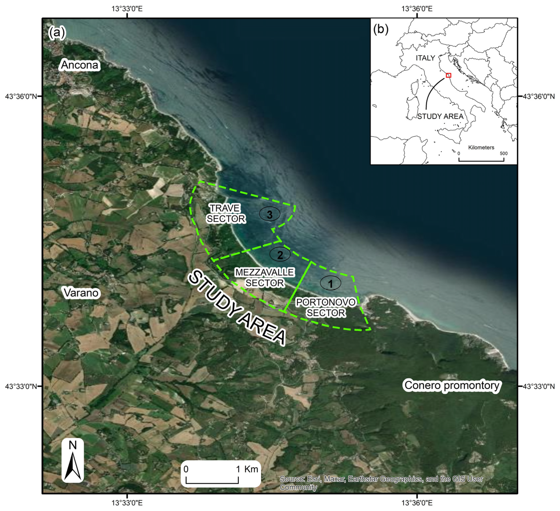
Figure 1. Map displaying the position of the study area: (a) Satellite image showing the study area and the three sectors called Portonovo, Mezzavalle and Trave. (image taken from GeoEye satellite database, 2020). (b) Location of the study area along the Italian Adriatic coast.
Remotesensing 16 02604 g001
Figure 2. Workflow sketch: (1) fieldwork; (2) data analyses and surveys. (3) Parameters’ extraction. (4) Machine learning analysis. (5) Slope stability analysis.
Remotesensing 16 02604 g002
Figure 3. Representation of Random Forest.
Remotesensing 16 02604 g003
Figure 4. Representation of eXtreme Gradient Boosting.
Remotesensing 16 02604 g004
Figure 5. Extracted sections are highlighted in violet and numbered. Sections used for the LEM analysis are represented in violet from 1–10.
Remotesensing 16 02604 g005
Figure 6. Geological/geomorphological setting of the study area and “Sectors”: (1) Portonovo; (2) Mezzavalle; (3) Trave. Bedrock legend: SCH (Schlier Fm., Lower Miocene-Upper Miocene), GNOa (Sapigno Fm. Upper Miocene), FCO (Colombacci Fm., Upper Miocene), Tv (Trave horizon, Lower Pliocene), FAA (Argille Azzurre Fm., Lower Pliocene-Lower Pleistocene).
Remotesensing 16 02604 g006
Figure 7. Pictures portraying the different configurations of the cliff base. (a) Portonovo sector; (b) Mezzavalle sector; (c) Trave sector.
Remotesensing 16 02604 g007
Figure 8. Horizontal georeferencing uncertainty, measured between the 1978 and 2022 orthophotos.
Remotesensing 16 02604 g008
Figure 9. NSM values calculated along transects, referring to the period 1978–2022: Portonovo and Trave sector showed the highest values of retreat. Computed transects (a) at Portonovo sector; (b) at Mezzavalle sector; (c) at Trave sector.
Remotesensing 16 02604 g009
Figure 10. ML results and analysis performed using RF and XGB algorithms. (1) Sketch displaying the parameters used in the analysis. (2) Illustration of the ML algorithm used. (3) Sketch illustrating ML results. (3a) Graph showing feature importance resulting from RF algorithm. (3b) Confusion matrix of RF elaboration. (3c) Graph illustrating the feature importance extracted using XGB algorithm. (3d) Confusion matrix of XGB analysis.
Remotesensing 16 02604 g010
Figure 11. Graph comparing FS and cliff height values in the ten extracted sections. The number below the dot refers to the section number in Table 5.
Remotesensing 16 02604 g011
Table 2. List of the parameters used for numerical modeling (refer to Figure 9 for the number of the transects reported).
Lithologyγ (KN/m3)GSImiDUCS (MPa)
Argille Azzurre Fm.
(228–265)
24357025
Faulted rocks
(266–276)
232540.620
Argille Azzurre Fm.
(277–290)
24357025
Argille Azzurre Fm.
(291–310)
24457030
Orizzonte del Trave 255017050
Table 3. Range of GSI and UCS values for the three sectors according to different transects.
SectorTransectsGSIUCS (MPa)
Portonovo1–795035
Mezzavalle80–18405
185–21501
Trave216–2274530
228–2653525
266–2762520
277–2903525
291–3104530
Table 4. DSAS results for each period analysed. Mean EPR and ECI are reported.
PeriodsPortonovoMezzavalleTrave
EPR (m/yr)ECI (m)EPR (m/yr)ECI (m)EPR (m/yr)ECI (m)
1978–2022−0.240.09−0.090.09−0.250.09
Table 5. Results from LEM analysis along the extracted sections.
SectionFSCliff Height (m)
12.0437
21.8642
31.5250
41.1273
51.2180
60.91120
71.1497
80.9860
92.2650
104.3725
Disclaimer/Publisher’s Note: The statements, opinions and data contained in all publications are solely those of the individual author(s) and contributor(s) and not of MDPI and/or the editor(s). MDPI and/or the editor(s) disclaim responsibility for any injury to people or property resulting from any ideas, methods, instructions or products referred to in the content.