Article

An Assessment of Changes in the Thermal Environment during the COVID-19 Lockdown: Case Studies from the Greenland and Norwegian Seas

College of Resources and Environment, Huazhong Agricultural University, Wuhan 430070, China
*
Author to whom correspondence should be addressed.
Remote Sens. 2024, 16(13), 2477; https://doi.org/10.3390/rs16132477
Submission received: 11 May 2024 / Revised: 20 June 2024 / Accepted: 1 July 2024 / Published: 6 July 2024
(This article belongs to the Section Urban Remote Sensing)

Abstract

:
The COVID-19 lockdown had a significant impact on human activities, reducing anthropogenic heat and CO2 emissions. To effectively assess the impact of the lockdown on the thermal environment, we used the sliding paired t-test, which we improved from the traditional sliding t-test by introducing the paired t-test for sliding statistical tests, to test the abrupt change in the thermal environment. Furthermore, an additive decomposition model and wavelet analysis method were used to analyze the characteristics of trend and irregular change, coherence, and phase difference of the time series data with respect to the thermal environment. We chose the Greenland Sea and the Norwegian Sea, regions highly sensitive to changes in climate and ocean circulation, as case studies and used remote sensing data of the sea surface temperature (SST) and the atmospheric CO2 concentration data obtained from the Goddard Earth Sciences Data and Information Services Center from January 2015 to December 2021 for the analysis. The results show that although the annual spatial mean SST in 2020 is lower than the mean of all 7 years in most areas of the two seas, there is no evidence of a significant mutation in the decrease in the SST during the lockdown in 2020 compared with the temperatures before, according to the sliding paired t-test. The analysis of the irregular components of the monthly mean SST decomposed by an additive decomposition model also does not show the anomalously low SST during the lockdown in 2020. In addition, the lockdown had almost no impact on the increasing trend of CO2 concentration. The wavelet analysis also shows that there is no obvious anomaly in coherence or phase difference between the periodic variation of the SST and the CO2 concentrations in 2020 compared with other years. These results suggest that the direct effect of the COVID-19 lockdown on the thermal environment of the study area could be negligible.

1. Introduction

COVID-19 broke out in late 2019 and spread rapidly in early 2020, which, at the time, was the most devastating health crisis entailing a high risk for the global health care system [1,2,3,4]. To restrict its spreading, the World Health Organization (WHO) and national governments repeatedly proposed a number of preventive methods, of which a lockdown was the most common and effective [5,6,7,8]. During the lockdown, people’s movement outside, industrial production, and all transport systems were severely restricted [9], which had a significant negative impact on the global economy [10,11]. However, it also provided an opportunity to investigate the impact of the restriction on the urban climate and the urban heat island effect [12], and even on the global thermal environment.
The restriction reduced industrial activities, the number of automobiles, and the large amount of man-made heat generated [13]. Anthropogenic heat emissions play an important role in the rise of urban temperatures. There is an estimate in Montreal City, Canada, that an 80% reduction in traffic volume equates to an approximately 1 °C reduction in near-surface temperature [14]. Meanwhile, emissions of air pollutants were also reduced [15,16], and environmental pollution is usually observed to be positively correlated with increases in land surface temperature (LST) and surface urban heat island intensity (SUHII). Therefore, the decrease in pollutant concentration, reduction of urban temperature, and alleviation of the urban heat island effect are presented simultaneously [17,18,19,20]. Additionally, normalized difference vegetation index (NDVI) usually has an inverse correlation with LST; during the lockdown, NDVI was significantly increased, which also contributed to the significant reduction of LST [21,22,23]. Determined by using remote sensing images, a reduction in the LST and SUHII of cities because of the confinement situation has been observed in many regions in comparison to the same dates in other years and 2020 without home confinement [24,25,26,27]. As reported, LST was reduced by 1–2 °C over Europe and North America [28] by 0.27–7.06 °C in some big cities of India [29], by an average of 4.6 °C in Andalusia, Spain [24], and by 14.7 °C in cold region cities of Turkey [20]. Also, it is found that the SUHII decreased by about 1–2 °C over Europe and North America [28], and by 1.02 °C in Andalusia, Spain [24]. As to the sea surface temperature (SST), it is influenced by multiple factors, including cloud cover, surface and advective heat fluxes, and atmospheric CO2 and aerosol concentrations; the impact of the lockdown on the SST may vary from region to region. Some studies reported that the SST rose in the Bay of Bengal and the Yellow Sea due to the lockdown [30,31], while other studies claimed that the SST reduced in regions such as the eastern Pacific and the north Indian Ocean [32,33].
The lockdown during the COVID-19 pandemic also led to a reduction in CO2 emissions in 2020. One European estimate shows that more than 195,600 thousand tons of CO2 were avoided during the first 6 months of 2020, compared to the same period of 2019, representing a decrease of 12.1% in emissions change [34]. Compared with mean levels of 2017–2019, India’s total fossil-based CO2 emissions by mid-June 2020 fell by 139 million tons [35]. At a global scale, the daily CO2 emissions decrease was estimated to be by 17% by early April 2020, compared with the mean 2019 levels [36]. In the first half of 2020, the decrease in global CO2 emissions was estimated to be 1551 Mt compared with the same period in 2019 [37]. Liu et al. [38] calculated from inventory and near-real-time activity data and found that the global reduction in CO2 emissions for the whole year of 2020 was 6.3% (2232 MtCO2) compared with 2019.
The above studies of the lockdown on LST, SUHII, SST, and CO2 emissions provide useful information on the impact of human activities on the thermal environment. However, most of these studies focus on the city scale and have little statistical testing of the significance of thermal environmental change. As for the impact of the lockdown on global thermal environment, previous studies mainly focused on the policies of climate change in the future [39,40,41]. Although there is an estimation of the direct effect of the lockdown on the cooling of the global climate simulated by the FaIR v1.5 climate emulator [42], the studies based on the observed data are few.
To this end, we aim to analyze whether there are significant changes in the thermal environment affected by the lockdown during 2020, which are further corroborated by analyzing the changes in the atmospheric CO2 concentration. So, we try to use the mutation test method to check whether there are abrupt changes in the thermal environment that are statistically significant. Among the mutation test methods, the Mann–Kendall (MK) mutation test is a common method to test the mutation in a time series, such as abrupt change analysis in temperature and precipitation [43,44,45,46], and drought and runoff [47,48,49,50], which are related to the thermal environment or climate. Also, the sliding t-test is widely used in these study areas [51,52,53,54]. The sea surface temperature (SST) significantly correlates with the global climate [55,56,57]. It responds to the changes in the Earth’s climate system and thermal environment. It can therefore be used for monitoring the state and detecting changes in the climate, and it is considered one of the climate change indicators [58]. Thus, we use SST as an indicator to assess the changes in the thermal environment during the COVID-19 lockdown. To make the analysis concrete, we chose the Greenland Sea and the Norwegian Sea as case studies and analyzed the SST characteristics over time. The Greenland Sea and Norwegian Sea play an important role in water exchange between the Arctic Ocean and the North Atlantic Ocean. The East Greenland Current carries Arctic sea ice and cold, low-salinity surface water for the Atlantic Ocean [59], whereas the Norwegian Atlantic Current carries the warm and salty Atlantic surface water for the Arctic Ocean [60]. Thus, these two seas are highly sensitive to changes in climate and ocean circulation, and changes in the thermal environment of the two seas not only reflect local changes but could to some extent represent changes on a global scale.
As the change in the thermal environment during the lockdown is the main focus, the monthly data of the SST and the atmospheric CO2 concentrations with respect to the study areas were used in this study. The MK mutation test is usually suitable for data without a seasonal cycle. Therefore, the sliding t-test method was a candidate for the abrupt change test in this study. Moreover, we introduced the paired t-test for the sliding statistical test and replaced the t-test in the sliding t-test with the paired t-test, thus, improving the traditional sliding t-test. By using the paired t-test, the improved sliding t-test method would be more sensitive in testing the abrupt change points in the time series of the seasonal data, as the paired t-test calculates each difference between the data of two samples in the same month and then tests the significance of the differences. Additionally, an additive decomposition model and the wavelet analysis method were used to analyze the characteristics of trend and irregular change, coherence, and phase difference of the time series data. The tool used to process the data analysis in this study is the free software R 4.1.3, and the R package WaveletComp 1.1 (https://CRAN.R-project.org/package=WaveletComp, accessed on 24 September 2023) was used for the wavelet analysis. Through the combined analysis of the SST and the atmospheric CO2 concentrations, the efforts of this work are intended to provide effective information about the impact of the COVID-19 lockdown, during 2020, on the thermal environment, as well as on global climate change.

2. Materials and Methods

2.1. Study Area and Data Source

The Greenland Sea and the Norwegian Sea are two, bordered seas between Greenland and Europe, bounded in the south by the Greenland–Iceland–Faeroe shallow transverse, in the north by the Arctic Ocean, and in the northeast by the Barents Sea (Figure 1). With the effect of the ocean currents, water from low and high latitudes meet and interact here. The region is an active area with frontal mixing, deep convective mixing, and conversion from light surface water to dense deep waters. Thus, large heat exchanges take place in this region [61], the thermal state of which can reflect the global climate change, and we analyze the thermal environment of the region using the indicator of SST, which was extracted from the “Sounder SIPS: AQUA AIRS IR-only Level 3 CLIMCAPS: Comprehensive Quality Control Gridded Monthly V2” (SNDRAQIL3CMCCP 2) dataset obtained from the Goddard Earth Sciences Data and Information Services Center (https://disc.gsfc.nasa.gov/, accessed on 22 September 2023). The SNDRAQIL3CMCCP 2 dataset is a remote sensing data product of the Atmospheric Infrared Sounder (AIRS), which is a grating spectrometer aboard the second Earth Observing System (EOS) polar-orbiting platform, EOS Aqua. The dataset is gridded with a spatial resolution of 1.0° × 1.0° and a monthly temporal resolution. We also analyze whether the lockdown affects the atmospheric CO2 concentration. This concentration was extracted from the “OCO-2 GEOS Level 3 monthly, 0.5° × 0.625° assimilated CO2 V10r” (OCO2_GEOS_L3CO2_MONTH) dataset, which was also obtained from the Goddard Earth Sciences Data and Information Services Center. The OCO2_GEOS_L3CO2_MONTH dataset is gridded with a spatial resolution of 0.5° × 0.625° and a monthly temporal resolution. In this study, we chose the period from January 2015 to December 2021 for the analysis, as atmospheric CO2 concentration data are available from January 2015 onwards.

2.2. Sliding Paired t-Test

Sliding t-test can be used to detect the mutation of a series. It slides a test whether the difference between the mean values of the two sequences is significant or not by using a t-test. However, as in this study the monthly mean SST and the monthly mean atmospheric CO2 concentration have seasonal variations, we improve the traditional sliding t-test method by using paired t-test for sliding statistical test, and use the improved sliding t-test, called sliding paired t-test in this study, to test the abrupt change. Suppose that the two sub-sequences with the same sample size of a time series before and after a test point are as follows:
X k 1 = x k m , x k m + 1 , , x k 1
and
X k = x k , x k + 1 , , x k + m 1 , k = m + 1 , m + 2 , , n m + 1 ,
where xk is the element of the analyzed time series at the test point k; m is the sample size of either sub-sequence; and n is the sample size of the entire time series. Then, we calculate the difference between each sample of Xk−1 and Xk as the following:
d k i = x k m + i 1 x k + i 1 , i = 1 , 2 , , m ,
where xkm+i−1 and xk+i−1 are the ith paired samples in Xk−1 and Xk, respectively. Thereafter, the test statistic t at the test point k is calculated as follows:
t k = d k ¯ s k / m ,
where d k ¯ and sk are, respectively, the mean and the standard deviation of the set consisting of the difference dki; and m is the sample size of Xk−1 and Xk. By changing the value of k from m + 1 to nm + 1, we have a series of the statistic t values at each test point k. If the p-value of the statistic tk with the m − 1 degrees of freedom is less than the significant level (0.05 for one tail), it means that the sequence before point k is significantly different from the sequence after point k. Then, we consider that there is a mutation at the test point.
In this study, when testing the mutation of the SST time series of the study area, xkm+i−1 and xk+i−1 in Equation (3) denote the monthly mean SST at the points km + i − 1 and k + i − 1 of the time series, respectively; when testing the mutation of the CO2 concentration time series over the study area, xkm+i−1 and xk+i−1 denote the monthly mean CO2 concentration at the points km + i − 1 and k + i − 1, respectively. The sample size of either sub-sequence m is taken as 12, so that the samples of the two tested sub-sequences are paired in the same month.

2.3. Additive Decomposition Model

Monthly data series usually contain a trend component and a seasonal component. The trend component reflects the series increasing or decreasing over a long time; the seasonal component reflects the character of repeating short-term cycle with equal time periods. As for monthly mean temperature, the time periods are 12 months, and the high values of temperature always occur in the summer months, while the low values always occur in the winter months. Therefore, each component obtained from the decomposition of a seasonal time series can give more useful underlying information rather than the original series. It is useful to see the general trend more clearly and facilitates the analysis of the periodic characteristics of the series.
The additive seasonal decomposition model, used in this study, describes an observed time series at time t as follows:
x t = T t + S t + e t ,
where x(t) denotes the monthly mean SST or the monthly mean atmospheric CO2 concentration, as determined by the time series of which is used for the decomposition analysis; T(t) is the trend component of the time series, calculated by using a centered moving average smoother; S(t) is the seasonal component, reflecting the contribution of the seasonal factors; and e(t) is the irregular component, also considered a random part for the model. According to Equation (5), T(t) accounts for the general trend change in the series, and S(t) accounts for the seasonal change in the series. Therefore, other factors affecting the series are represented in e(t), which is considered a random part or random noise for the model as it cannot be explained by the general trend factor and the seasonal factors. These factors can be random events, unexpected occurrences, etc.
In this study, the order of the centered moving average smoother used to estimate the trend component T(t) is 12, which corresponds to the number of months with respect to the seasonal span. The detailed steps of the decomposition in the study are as follows:
(1)
Calculate the trend component using a centered moving average of order 12, which can be written as follows:
T t = 1 24 x t 6 + 1 12 i = 5 5 x t + i + 1 24 x t + 6 .
(2)
Calculate the detrended series using the following:
D t = x t T t .
(3)
Estimate the seasonal component for each month by averaging the detrended values for that month. For example, the seasonal component S(t) for January is the average of all the January values in the series of D(t). Thus, The S(t) repeats with a fixed periodicity of 12, i.e., S(t) = S(t + 12).
(4)
Calculate the irregular component using:
e t = x t T t S t .
From Equation (6), it can be seen that 1/12 of the observed value x(t) contributes to the trend T(t). If the COVID-19 lockdown caused anomalies in SST or CO2 concentration, a small part of the anomalies would be presented in the trend component. Since the seasonal component is the same for all the same months throughout the series, according to Equation (8), the remaining large part of the anomalies would be presented in the irregular component.

2.4. Wavelet Analysis

Wavelet transform is a useful tool for multiresolution analysis through dividing a given function or a signal into different scale components. It can express an arbitrary function on multiresolution approximation spaces [62], decomposing the whole function space into subspaces at different scales, and then provide useful information in localization and at matched scales. By using the wavelet method in this study, it is possible to focus on the local temporal characteristics of the thermal environment with respect to the study area, thus providing information on whether there are significant differences that exist during the period of lockdown compared with periods without a lockdown. To more effectively analyze the localized variations, we use the detrended series of monthly mean SST and the detrended series of monthly mean atmospheric CO2 concentration for analysis. According to Equations (5) and (7), the detrended part, consisting of the seasonal component and the irregular component, can also be expressed as follows:
D t = S t + e t
The continuous wavelet transform, by projecting the analyzed function D(t) on a wavelet function with respect to ψ(u), is defined as follows:
W D s , τ = + D t 1 s ψ * t τ s d t ,
where * denotes the operation of complex conjugation; s is a scaling factor that controls the width of the wavelet; and τ is a translation parameter that indicates the central location of the wavelet, implying a translation or shift of the function.
Among several wavelet functions available, Morlet wavelet is frequently used, and it is also used in this study. The function is defined as follows:
ψ η = π 1 / 4 e i ω 0 η e η 2 / 2 .
When dealing with the discrete series of the detrended part {D(n), n = 1, …, N} with N observations, the integral in Equation (10) is easily discretized as follows:
W n D s = δ t s m = 1 N D m ψ * m n δ t s ,
where δt is a uniform step.
Cross wavelet transform is a powerful tool for analyzing the synchronicity of two time series, allowing wavelet coherence and phase difference to be derived [63,64,65,66]. Wavelet coherence is able to indicate the common power of two variables, being in this way similar to a correlation coefficient [67]. The phase difference could describe the relation of the move characteristic between the two series.
Suppose that the two series used for cross-relation analysis are
D 1 = D 1 n
and
D 2 = D 2 n .
The cross wavelet transform of them is defined as follows:
W n 12 = W n D 1 W n D 2 * .
When D1 = D2,
W n 11 = W n D 1 W n D 1 * = W n D 1 2 .
Next, the complex wavelet coherence of the two series is defined as follows [68]:
ϱ n 12 = S W n 12 S W n 11 S W n 22 ,
where S denotes a smoothing operator in both location and scale.
Thereafter, the wavelet coherence of the two series is simply the absolute value of the complex wavelet coherence, defined with a value between 0 and 1; that is calculated as follows:
R n 12 = ϱ n 12 .
Then, the phase difference of the two series is the complex argument of the cross wavelet transform; that is calculated as follows:
ϕ n 12 = arg W n 12
The phase difference is in the range from −π to π. It can imply that the two series x and y move in phase or in anti-phase, and that one leads the other.
In addition, the statistical significance of the coherence and the phase difference derived by the cross wavelet transform analysis were evaluated. They provide information about the time intervals and periods at which the coherence and the phase difference are significant. In this study, we used the cross wavelet transform to analyze the wavelet coherence and the phase difference between the SST of the Greenland Sea and the Norwegian Sea. In this case, D1 in Equation (13) denotes the time series of the monthly mean SST of the Greenland Sea, and D2 in Equation (14) denotes that of the Norwegian Sea. We also performed a cross wavelet transform analysis between the monthly mean SST of the two seas and the monthly mean atmospheric CO2 concentrations over the two seas. This time, D1, denotes the time series of the monthly mean SST, and D2 denotes the time series of the monthly mean atmospheric CO2 concentration. If there are abrupt changes in the SST of the two seas during the lockdown in 2020, it would be presented in the results of the coherence and the phase difference.

3. Results

3.1. Change Characteristics of the SST

3.1.1. Spatial Distribution of the Annual SST

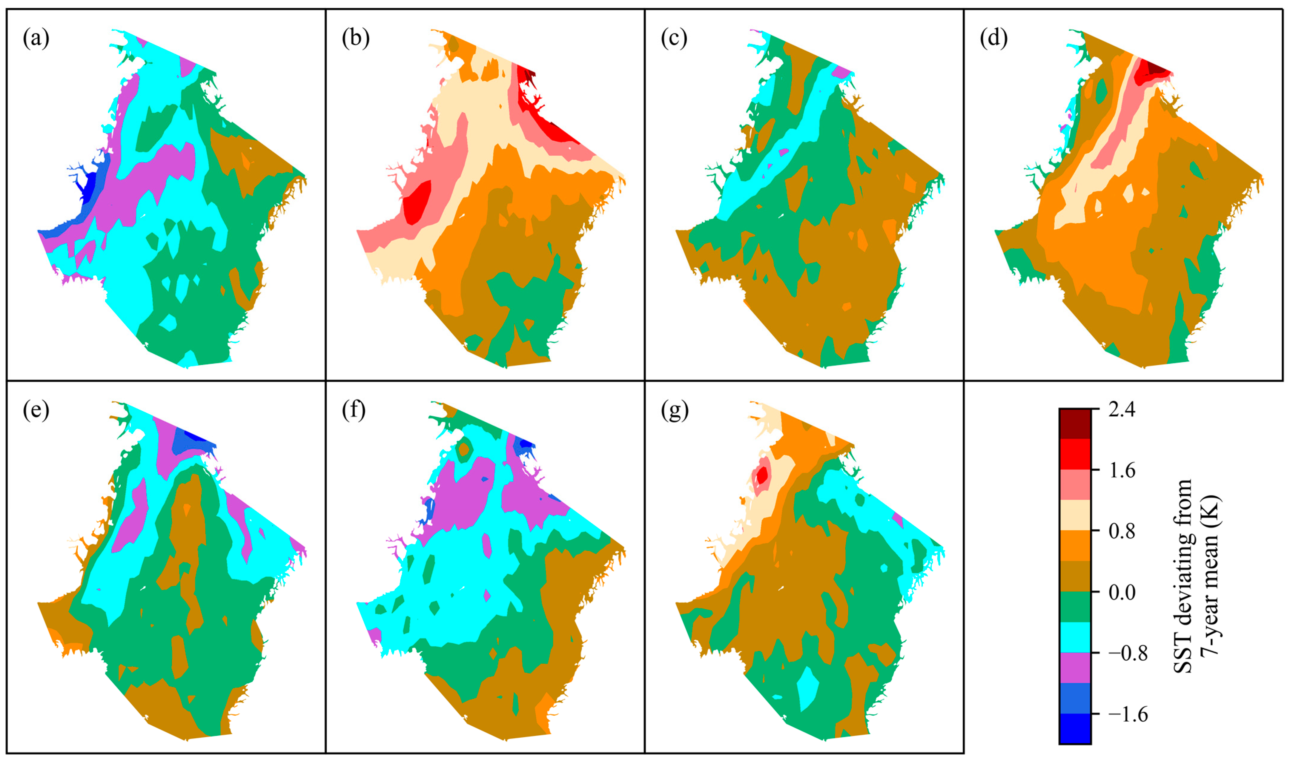
We calculated the annual mean SST from 2015 to 2021 and the mean of all 7 years for each grid point of the Greenland Sea and the Norwegian Sea. Then, we evaluated the differences between the mean of each year and the mean of all 7 years in SST. The results are displayed in Figure 2. It can be seen that the SST of most areas of the two seas in 2020 is lower than the mean of all 7 years. Only some parts of the Norwegian Sea and very small parts of the Greenland Sea have slightly greater temperatures than the mean of the 7 years. However, the temperatures of most areas in 2019 are also below the mean of the 7 years, although the area with a temperature difference of less than −0.4 K is smaller than that in 2020. Additionally, the area with a temperature lower than the mean of all 7 years is larger in 2015 than in 2020.

3.1.2. Sliding Paired t-Test Results of the SST

We further calculated the monthly mean SST of the entire Greenland Sea and the entire Norwegian Sea from January 2015 to December 2021. The results show that there is no obvious temperature anomaly in 2020 compared with other years (Figure 3). Although the temperature of the Norwegian Sea in March 2020 is the lowest in the analysis period, with a value of 271.5 K, the second lowest temperature is 272.1 K in February 2015, which is only 0.6 K higher. As for the Greenland Sea, the temperature in March 2020 is the second lowest with 256.8 K; the lowest temperature is in February 2015, which is 0.1 K lower (256.7 K).
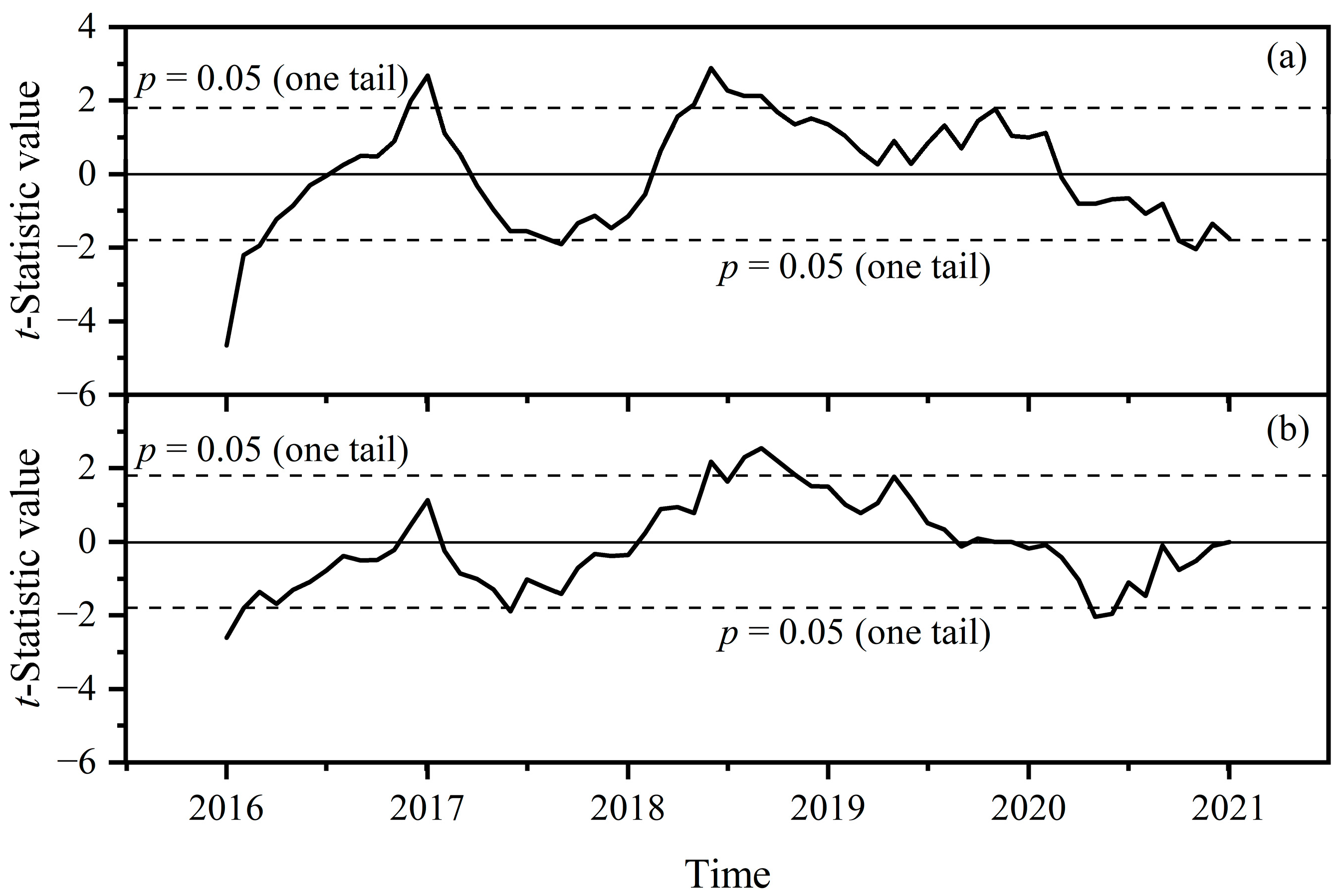
We then performed the sliding paired t-test with the two monthly mean SST series, the results of which are shown in Figure 4. It can be seen in 2020 that there are two significant abrupt changes with respect to the Norwegian Sea, in May and July, and that there are also two significant abrupt changes with respect to the Greenland Sea, in October and November. However, these abrupt changes indicate mutations of increase, which means that the temperatures before are lower than the temperatures after, because the t-statistic values are negative. This might be explained by the fact that the global economy was gradually recovering. Thus, the temperature before the mutation was lower due to the lockdown. However, as can be seen in Figure 4, there is no evidence of significant mutation in temperature decrease in 2020 compared with the temperature before. Conversely, there are some significant mutations in temperature decrease in other years. These mutations are in December 2016, January 2017, and from May to September 2018, with respect to the Greenland Sea; and in June, and from August to November 2018, with respect to the Norwegian Sea.

3.1.3. Decomposition Analysis of the SST

We further took the decomposition of the monthly mean SST series of the two seas by using an additive seasonal decomposition model described in Equation (5), in which the monthly mean SST is considered as x(t). The trend components (i.e., T(t) in Equation (5)) of the monthly mean SST series of the two seas are illustrated in Figure 5. The trend of the Greenland Sea is in the range from 265.8 K to 267.8 K, spanning 2.0 K; the trend of the Norwegian Sea is in the range from 275.3 K to 276.2 K, spanning less than 1.0 K. Furthermore, we performed linear regression with the trends of the temperatures, using the number of months since July 2015 as the explanatory variable. The regression results are shown in Table 1. All the coefficients of the regression are significant. According to the regression models, the temperature trend of the Greenland Sea is decreasing by 0.0097 K per month from July 2015 to June 2021, and that of the Norwegian Sea is decreasing by 0.0036 K per month. However, the coefficients of the determination suggest that the linear regression models can only explain 14.5% of the variation on the temperature trend of the Greenland Sea and 10.8% of the Norwegian Sea, which indicates that the global linear model is not sufficient to explain the SST trends of both seas.
Thereafter, we performed locally weighted linear regression with the trends. This time, the coefficients of the determination with respect to the Greenland Sea and the Norwegian Sea are 0.962 and 0.966, respectively, which indicate that the locally weighted linear regression models could explain the temperature trends well. The fitted lines of these models are also illustrated in Figure 5. According to the fitted lines, it can be seen that the temperature trend of the Greenland Sea is generally decreasing from February 2018 to April 2020 and then starts to increase until the end of analyzed period. However, in May and June 2020, the world is still in a state of mass lockdown. As to the Norwegian Sea, the temperature is even in a general increasing trend from November 2019 to November 2020, which covers the period of the most restricted lockdown. These results also suggest that the lockdown might not be the main factor causing the temperatures of the two seas to be lower than the mean of the 7 years in 2020.
Additionally, the irregular components (i.e., e(t) in Equation (5)) of the two monthly mean SST series are presented in Figure 6 to see whether there is any anomaly. The 95% confidence intervals of the distributions for the irregular components are also shown in Figure 6. It can be seen that there are only four points out of the 95% confidence interval, with respect to the Greenland Sea (Figure 6a), of which two points are below the lower limit of the 95% confidence interval. These two points are for January 2017 and February 2020, and the January 2017 point is even lower than that of February 2020. However, by the end of February 2020, only China had a lockdown. From 10 March, Italy enforced a nationwide lockdown. Thereafter, other European countries began to implement lockdowns or restrictions. From 24 March, India commenced a lockdown with a total ban on venturing out of homes. In Russia, residents were ordered to stay at home from 30 March. By early April, nearly half of the states in USA directed residents to stay at home. The extent of the lockdown throughout the world in April and May reached the largest in 2020. Conversely, the irregular components of April and May 2020 had positive values. As for the Norwegian Sea (Figure 6b), there are four points out of the 95% confidence interval, of which only one point is below the lower limit of the 95% confidence interval. This point is June 2018. For 2020, the points of March, April, and May are still some distance from the lower limit of the 95% confidence interval. Oppositely, the point of June 2020 is above the upper limit of the 95% confidence interval. The analysis of the irregular components of the monthly mean SST also does not support the anomalously low SST during the lockdown in 2020.

3.2. Change Characteristics of the CO2 Concentration

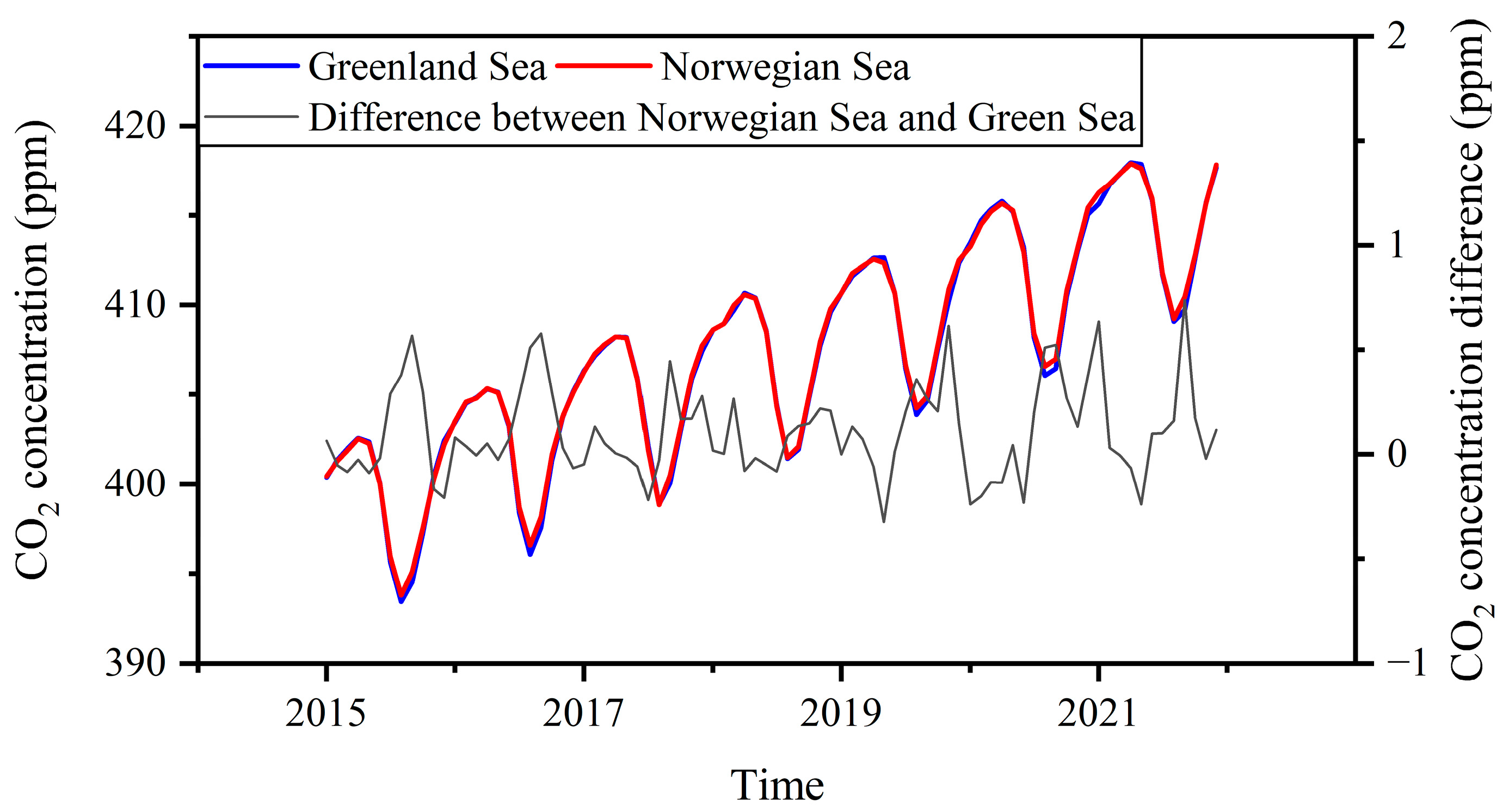
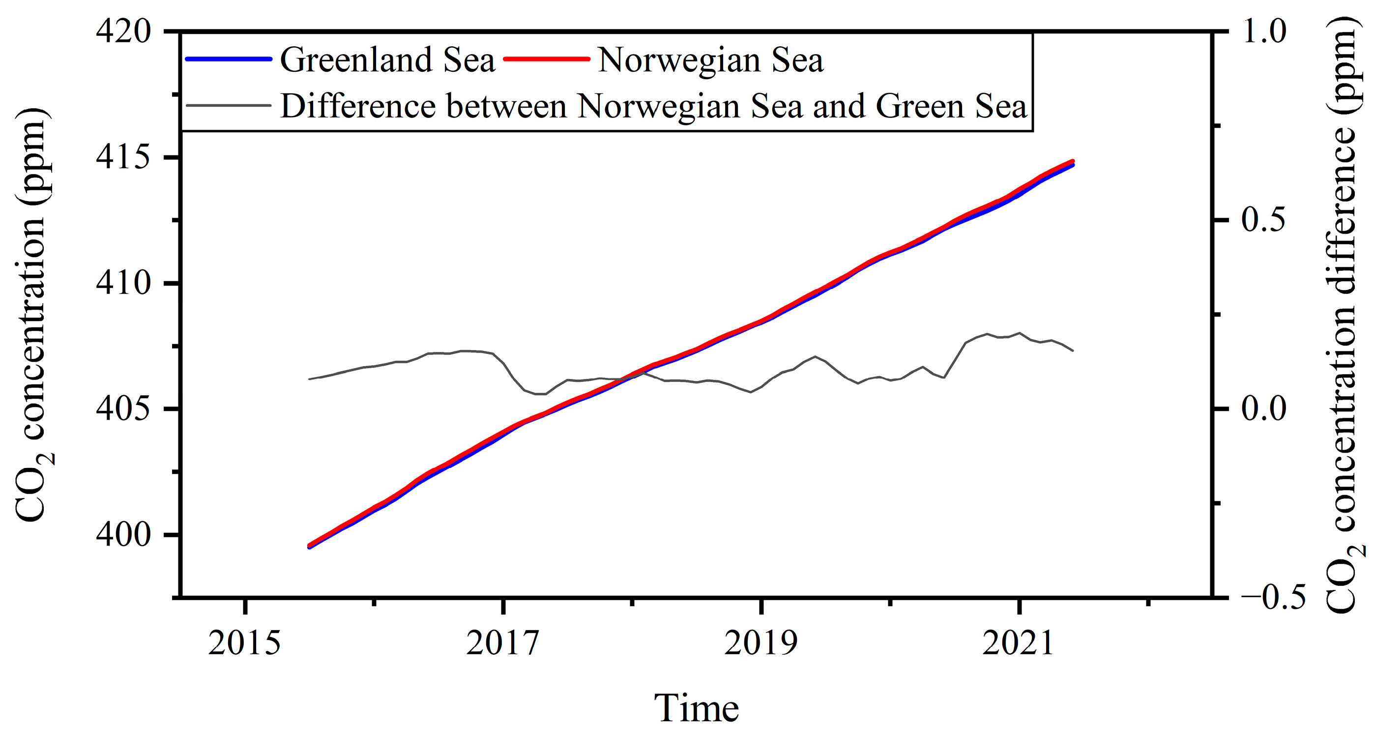
The monthly mean atmospheric CO2 concentrations over the whole Greenland Sea and the whole Norwegian Sea from January 2015 to December 2021 are shown in Figure 7. The concentrations with respect to the two seas are almost identical, with the two concentration curves overlapping almost completely. Figure 7 also shows the differences between the CO2 concentrations over the two seas, i.e., the concentrations over the Norwegian Sea minus those over the Greenland Sea. It can be seen that the absolute values of the difference are all less than 0.74 ppm, mostly less than 0.5 ppm. As can be seen from Figure 7, although the CO2 concentrations over the two seas rise and fall month by month over time, they appear to be increasing in a spiral.
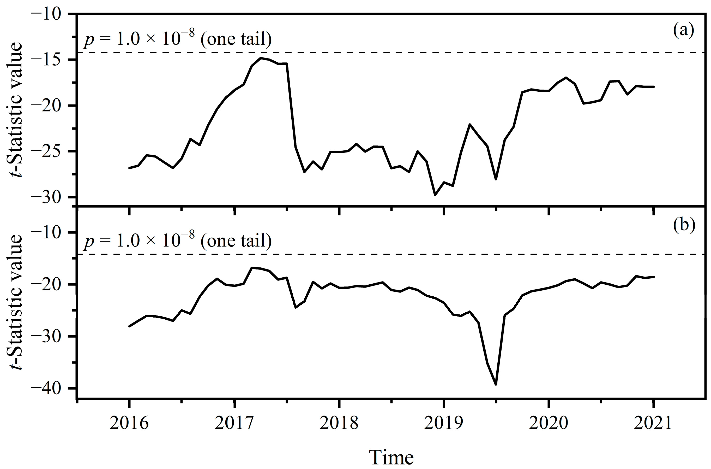
A sliding paired t-test was then performed on each of the two concentration series, the results of which are shown in Figure 8. It can be seen that the t-statistic values are always negative, and the absolute values are greater than 10, which means that over time, the CO2 concentrations 12 months later are always greater than the concentration 12 months before, with extreme statistical significance. The absolute values of the t-statistic in 2020 are almost no smaller than those of the last few months of 2019, which means that the lockdown in 2020 had almost no impact on the increase trend of the CO2 concentration, although the reductions in CO2 emissions are substantial.
The trends decomposed from the two CO2 concentration series are illustrated in Figure 9. It can be seen that the trends are almost straight lines. We further perform linear regression analyses on the CO2 concentrations of the trends, using the number of months since July 2015 as the explanatory variable. The regression results are shown in Table 2. All coefficients of the regression are extremely significant. Moreover, the coefficients of the determination are very high, with only 0.2% of the variation on the CO2 concentration trends that cannot be explained by the linear regression model. The rate of increase of the CO2 concentrations trends in the atmosphere over the two seas is almost the same, 0.207 ppm per month for the Greenland Sea and 0.208 for the Norwegian Sea.
Analyzed in conjunction with the temperature trend analysis above, the increasing trend in CO2 concentration does not appear to have an impact on the trend in SST, which does not appear to be increasing, or even slightly decreasing. Theoretically, the increase in CO2 concentration will cause the temperature to rise because the greenhouse effect is increasing. This result suggests that the effect of the CO2 concentration with an increasing rate of about 0.2 ppm per month on the temperature may not appear in a short period like the period analyzed in the study.
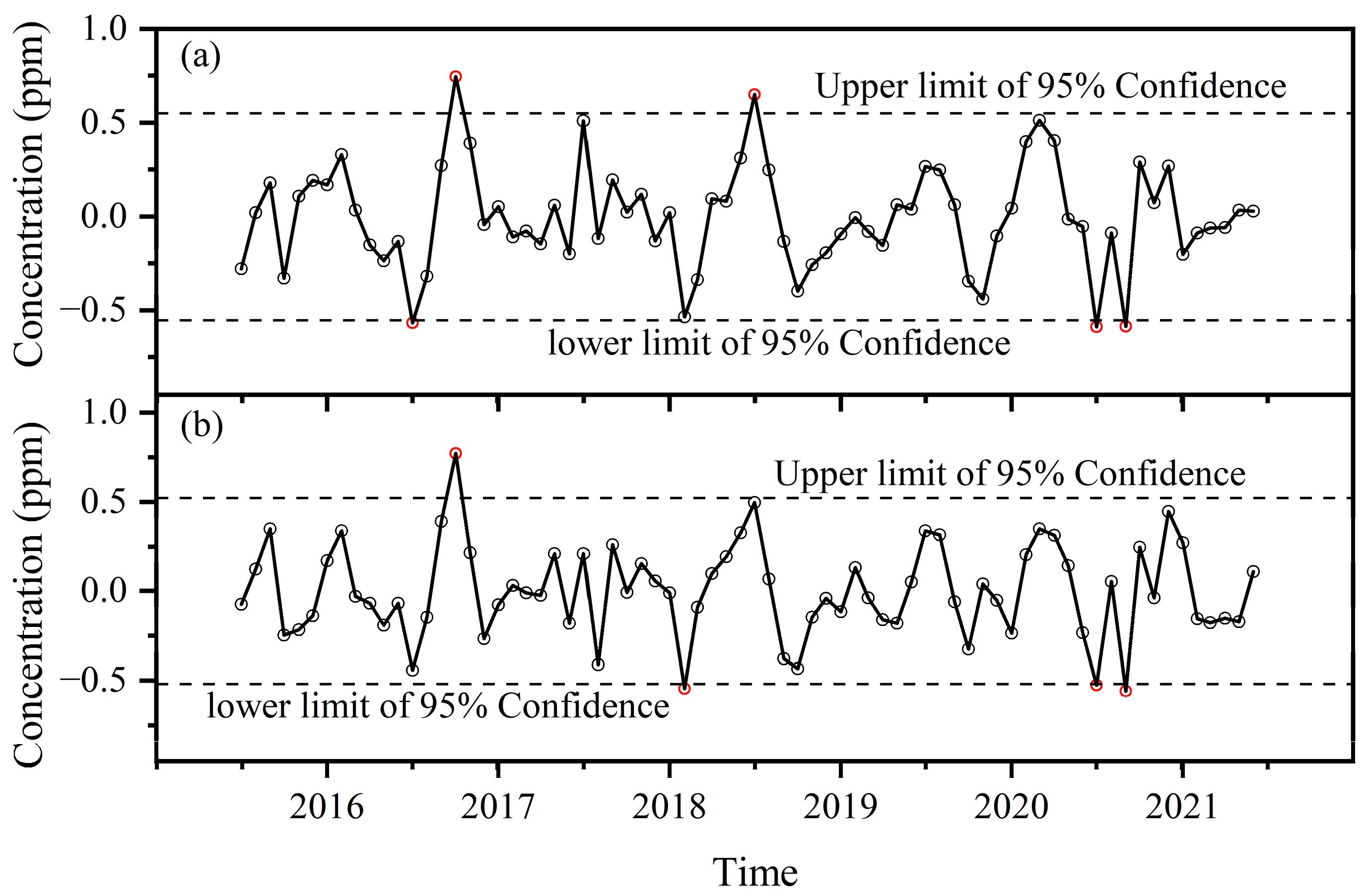
In addition, the irregular components of the two monthly mean CO2 concentration series are shown in Figure 10. Although in July and September 2020, the values of the irregular components about the two seas are blow the lower limit of the 95% confidence interval, those in April and May 2020, when the extent of the lockdown are largest throughout 2020, are greater than zero or very close to zero. If it is considered that the effect of the lockdown on the reduction in CO2 concentration is lagging, it is difficult to explain that the values of the irregular components about the two seas in August 2020 are very close to zero or even a little greater than zero. Moreover, the amplitude of all the irregular components deviating from zero is very small. For the Greenland Sea, the minimum value is −0.59 ppm, and the maximum value is 0.75 ppm; For the Norwegian Sea, the minimum value is −0.56 ppm, and the maximum value is 0.77 ppm. Combined with the trend analysis of the CO2 concentration, it also implies that the lockdown in 2020 had almost no effect in reducing the atmospheric CO2 concentration.

3.3. Relationships of the Periodic Variation

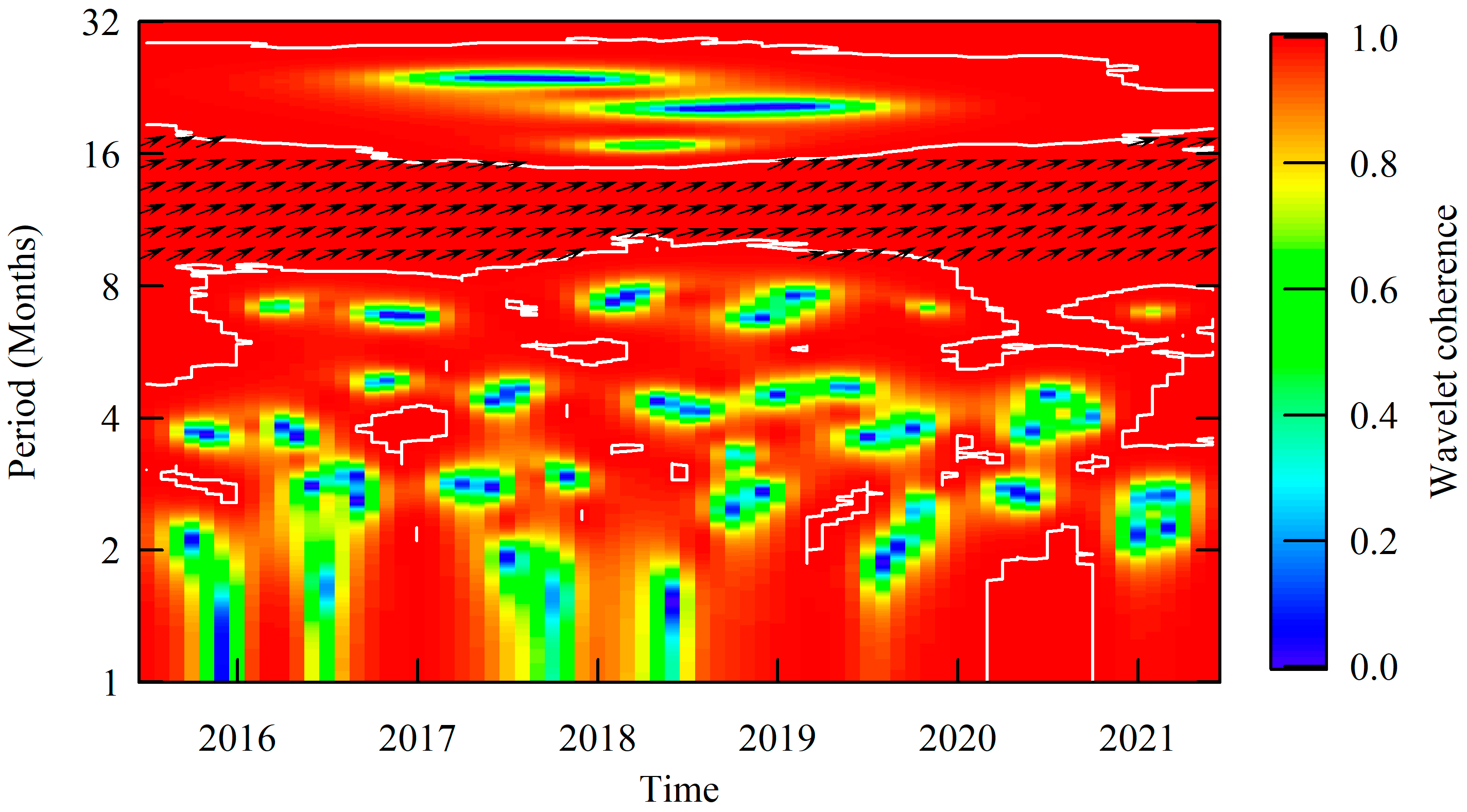
The cross-correlation between the detrended monthly mean SST of the Greenland Sea and the Norwegian Sea was analyzed using the wavelet method, which is shown in Figure 11. It can be seen that the coherence of two detrended series at periods of around 12 months is significant (significance level at 0.05) over the entire time interval from July 2015 to June 2021 and with very high values, very close to 1.0, indicating that the SST of the two seas is highly correlated at the scale of about 12 months. The phase difference between the two series is also illustrated in Figure 11 (phase for the Greenland Sea over that for the Norwegian Sea); only the phase difference that is significant (significance level at 0.05) is shown with an arrow. At periods of around 12 months, the phase difference is significant over the entire time interval, and the angle of the arrows is greater than 0 and less than π/2. Additionally, there is almost no difference from July 2015 to June 2021. These indicate that the SST of the two seas is changing in phase and with very high coherence, and that the change in SST of the Greenland Sea is leading while that of the Norwegian Sea is lagging.
Combining this analysis with Figure 3, it can be seen that the peak of the monthly mean SST of the Greenland Sea precedes that of the Norwegian Sea, i.e., when the monthly mean SST of the Greenland Sea starts to decrease from the highest of the year, the monthly mean SST of the Norwegian Sea still increases for a short period. This phenomenon could be explained by the ocean current. The East Greenland Current, a cold flow of water originating in the Arctic Ocean and flowing southward and southwestward along the east coast of Greenland, flows into the Greenland Sea [69], and then the outflow from the Greenland Sea flows into the Norwegian Sea [70]. This suggests that water masses are mainly transported from the Greenland Sea to the Norwegian Sea [71]. Therefore, the current reaching the Norwegian Sea is later than that reaching the Greenland Sea, which causes the SST of the Greenland Sea to change before that of the Norwegian Sea.
We further analyzed the periodic variation of the SST of the two seas with atmospheric CO2 concentrations. Figure 12 shows the cross-correlation between the detrended surface temperatures of the Greenland Sea and the detrended CO2 concentration over the Greenland Sea. At the periods of around 12 months, the coherence of these two detrended series is also significant (significance level at 0.05) and very close to 1.0. As to the difference in phase, the angle is in the range from −π to −π/2. This means that the SST of the Greenland Sea and the CO2 concentration over it are changing in anti-phase within a year, and that the SST is leading while CO2 concentration is lagging. For the Norwegian Sea, the character of the cross-correlation between the SST and the atmospheric CO2 concentration is very similar to that for the Greenland Sea except that the angle of the phase difference is much closer to −π (Figure 13). Focusing on the year 2020, it can be seen that there is no obvious anomaly in coherence and phase difference when looking at the periodic variation of the SST with the CO2 concentrations for the two seas compared with other years, which also implies that the lockdown in 2020 had almost no impact on the relationship between SST and atmospheric CO2 concentration. Since the lockdown in 2020 had almost no impact on the increase in CO2 concentration, as suggested by the above sliding paired t-test analysis and the combination of trend analysis and irregular component analysis performed by additive decomposition model, it could also mean that the lockdown had no significant effect on the SST of the two seas.

4. Discussion

The result of this study suggests that the lockdown during 2020 had little impact on the SST of the Greenland Sea and the Norwegian Sea. As to the global thermal environment, the impact might be extremely small. This may sound strange, as previous studies reported that LST and SUHII were reduced during the lockdown [24,25,26,27,28,29]. Just looking at the values, our results also show that the SST in 2020 is lower than the mean SST from 2015 to 2021, and the SST in either 2019 or 2021. However, when it comes to the effect of the lockdown on the thermal environment, the contribution of the lockdown in reducing the thermal environment may be overestimated. The fact that the temperatures in the first months of 2020 were lower than in 2019 could be a normal phenomenon, just a normal variation of the thermal environment. In fact, the SST in 2015 was even lower than in 2020. Further analysis of our study suggests that the lower SST during the lockdown in 2020 is not an abrupt change, according to the sliding paired t-test; the locally weighted linear fit with the trends of the SST shows that the Greenland Sea SST trend is generally decreasing from February 2018 to April 2020 and that the Norwegian Sea SST trend is generally decreasing from February 2018 to November 2019. It is also argued by Forster et al. [42] that the direct effect of the pandemic-driven response on the global climate will be negligible, with a cooling of around 0.01 °C by 2030 compared to a baseline scenario that follows current national policies.
It is generally accepted that the Earth is becoming warmer and that sea surface temperatures are generally increasing, but in some short periods SST can show a decreasing trend. Figure 14a shows the change in the average surface temperature of the world’s oceans since 1880 (https://www.epa.gov/climate-indicators/climate-change-indicators-sea-surface-temperature, accessed on 2 May 2024), using the 1971 to 2000 average as a baseline for depicting change. It is obvious that the general trend of the SST from 1880 to 2020 is increasing, and from 1901 through 2020, SST rose at an average rate of 0.078 K per decade. However, when focusing on short periods, such as 2001 to 2008 and 2015 to 2020, the trend is decreasing (Figure 14b,c). This is consistent with the results of our study, where the trends of the SST in the Greenland Sea and the Norwegian Sea from July 2015 to June 2021 are decreasing (Figure 5). In addition, Yang et al. presented that the overall warming trend of the Arctic SST is not obvious [72]. Furthermore, it is shown that the convection in the Greenland Sea declined from 2015 onward [73], which also had an effect on the heat exchange into the Greenland Sea. However, this local trend during the period does not affect the main conclusions of this study, as we focus mainly on the anomalous change in the thermal environment during the lockdown in 2020.

5. Conclusions

In light of the fact that the lockdown reduced the emission of greenhouse gases and may have an impact on the global thermal environment, this study analyzed the change characteristics of the SST of the Greenland Sea and the Norwegian Sea and the atmospheric CO2 concentration over the two seas from January 2015 to December 2021. The spatial distribution of the SST shows that its annual mean in 2020 is lower than the mean of all 7 years in most areas of the two seas, but there are still other years comparable to 2020 with temperatures lower than the 7-year mean. Furthermore, the sliding paired t-test on the monthly mean SST of the entire regions of the two seas shows that there is no significant mutation in temperature decrease in 2020, suggesting that the lower SST during the lockdown in 2020 is not an abrupt change; the locally weighted linear fit with the trends of the SST shows that the Greenland Sea SST trend is generally decreasing from February 2018 to April 2020 and that the Norwegian Sea SST trend is generally decreasing from February 2018 to November 2019. Focusing on the period during the lockdown, the SST trend of the Greenland Sea is not always decreasing, while the SST trend of the Norwegian Sea is even increasing. In addition, the analysis of the irregular components of the monthly mean SST also does not show the anomalously low SST during the lockdown in 2020.
As for the atmospheric CO2 concentrations over the two seas, the sliding paired t-test and their extracted trends indicate that they are steadily increasing and do not seem to be affected by the lockdown in 2020. Additionally, the cross-correlation analysis between the SST and the CO2 concentration, performed by the wavelet method, also shows that there is no obvious anomaly in coherence or phase difference in 2020 when compared with other years. These results suggest that the impact of the COVID-19 lockdown in 2020 on the thermal environment of the study area is insignificant and could be negligible.

Author Contributions

Conceptualization, methodology, and writing of the article, W.S.; collecting materials, X.Z.; verification of the results, H.Z. All authors have read and agreed to the published version of the manuscript.

Funding

This research was funded by the National Natural Science Foundation of China (NSFC), grant number 41701179.

Data Availability Statement

The original contributions presented in the study are included in the article, further inquiries can be directed to the corresponding author.

Conflicts of Interest

The authors declare no conflicts of interest.

References

  1. Giannopoulou, I.; Tsobanoglou, G.O. COVID-19 pandemic: Challenges and opportunities for the Greek health care system. Ir. J. Psychol. Med. 2020, 37, 226–230. [Google Scholar] [CrossRef] [PubMed]
  2. Jeffery, M.M.; D’Onofrio, G.; Paek, H.; Platts-Mills, T.F.; Soares, W.E., III; Hoppe, J.A.; Genes, N.; Nath, B.; Melnick, E.R. Trends in Emergency Department Visits and Hospital Admissions in Health Care Systems in 5 States in the First Months of the COVID-19 Pandemic in the US. JAMA Intern. Med. 2020, 180, 1328–1333. [Google Scholar] [CrossRef] [PubMed]
  3. Davin-Casalena, B.; Jardin, M.; Guerrera, H.; Mabille, J.; Trehard, H.; Lapalus, D.; Menager, C.; Nauleau, S.; Cassaro, V.; Verger, P.; et al. The impact of the COVID-19 pandemic on first-line primary care in southeastern France: Feedback on the implementation of a real-time monitoring system based on regional health insurance data. Rev. D Epidemiol. Sante Publique 2021, 69, 105–115. [Google Scholar] [CrossRef] [PubMed]
  4. Filip, R.; Gheorghita Puscaselu, R.; Anchidin-Norocel, L.; Dimian, M.; Savage, W.K. Global Challenges to Public Health Care Systems during the COVID-19 Pandemic: A Review of Pandemic Measures and Problems. J. Pers. Med. 2022, 12, 1295. [Google Scholar] [CrossRef] [PubMed]
  5. Atalan, A. Is the lockdown important to prevent the COVID-19 pandemic? Effects on psychology, environment and economy-perspective. Ann. Med. Surg. 2020, 56, 38–42. [Google Scholar] [CrossRef] [PubMed]
  6. Wong, C.K.H.; Wong, J.Y.H.; Tang, E.H.M.; Au, C.H.; Lau, K.T.K.; Wai, A.K.C. Impact of National Containment Measures on Decelerating the Increase in Daily New Cases of COVID-19 in 54 Countries and 4 Epicenters of the Pandemic: Comparative Observational Study. J. Med. Internet Res. 2020, 22, e19904. [Google Scholar] [CrossRef] [PubMed]
  7. Violato, C.; Violato, E.M.; Violato, E.M. Impact of the stringency of lockdown measures on COVID-19: A theoretical model of a pandemic. PLoS ONE 2021, 16, e0258205. [Google Scholar] [CrossRef]
  8. Sun, K.S.; Lau, T.S.M.; Yeoh, E.K.; Chung, V.C.H.; Leung, Y.S.; Yam, C.H.K.; Hung, C.T. Effectiveness of different types and levels of social distancing measures: A scoping review of global evidence from earlier stage of COVID-19 pandemic. BMJ Open 2022, 12, e053938. [Google Scholar] [CrossRef]
  9. Rupani, P.F.; Nilashi, M.; Abumalloh, R.A.; Asadi, S.; Samad, S.; Wang, S. Coronavirus pandemic (COVID-19) and its natural environmental impacts. Int. J. Environ. Sci. Technol. 2020, 17, 4655–4666. [Google Scholar] [CrossRef]
  10. Verschuur, J.; Koks, E.E.; Hall, J.W. Global economic impacts of COVID-19 lockdown measures stand out in high-frequency shipping data. PLoS ONE 2021, 16, e0248818. [Google Scholar] [CrossRef]
  11. Wu, J.; Zhan, X.; Xu, H.; Ma, C. The economic impacts of COVID-19 and city lockdown: Early evidence from China. Struct. Chang. Econ. Dyn. 2023, 65, 151–165. [Google Scholar] [CrossRef]
  12. El Kenawy, A.M.; Lopez-Moreno, J.I.; McCabe, M.F.; Domínguez-Castro, F.; Peña-Angulo, D.; Gaber, I.M.; Alqasemi, A.S.; Al Kindi, K.M.; Al-Awadhi, T.; Hereher, M.E.; et al. The impact of COVID-19 lockdowns on surface urban heat island changes and air-quality improvements across 21 major cities in the Middle East. Environ. Pollut. 2021, 288, 117802. [Google Scholar] [CrossRef] [PubMed]
  13. Sun, S.L.; Zhou, D.C.; Chen, H.S.; Li, J.J.; Ren, Y.J.; Liao, H.; Liu, Y.B. Decreases in the urban heat island effect during the Coronavirus Disease 2019 (COVID-19) lockdown in Wuhan, China: Observational evidence. Int. J. Climatol. 2022, 42, 8792–8803. [Google Scholar]
  14. Teufel, B.; Sushama, L.; Poitras, V.; Dukhan, T.; Bélair, S.; Miranda-Moreno, L.; Sun, L.J.; Sasmito, A.P.; Bitsuamlak, G. Impact of COVID-19-Related Traffic Slowdown on Urban Heat Characteristics. Atmosphere 2021, 12, 13. [Google Scholar] [CrossRef]
  15. Ali, G.; Abbas, S.; Qamer, F.M.; Wong, M.S.; Rasul, G.; Irteza, S.M.; Shahzad, N. Environmental impacts of shifts in energy, emissions, and urban heat island during the COVID-19 lockdown across Pakistan. J. Clean Prod. 2021, 291, 12. [Google Scholar] [CrossRef] [PubMed]
  16. Jephcote, C.; Hansell, A.L.; Adams, K.; Gulliver, J. Changes in air quality during COVID-19 ‘lockdown’ in the United Kingdom. Environ. Pollut. 2021, 272, 11. [Google Scholar] [CrossRef] [PubMed]
  17. Ghosh, S.; Das, A.; Hembram, T.K.; Saha, S.; Pradhan, B.; Alamri, A.M. Impact of COVID-19 Induced Lockdown on Environmental Quality in Four Indian Megacities Using Landsat 8 OLI and TIRS-Derived Data and Mamdani Fuzzy Logic Modelling Approach. Sustainability 2020, 12, 5464. [Google Scholar] [CrossRef]
  18. Mandal, I.; Pal, S. COVID-19 pandemic persuaded lockdown effects on environment over stone and areas. Sci. Total Environ. 2020, 732, 10. [Google Scholar] [CrossRef] [PubMed]
  19. Pal, S.C.; Chowdhuri, I.; Saha, A.; Ghosh, M.; Roy, P.; Das, B.; Chakrabortty, R.; Shit, M. COVID-19 strict lockdown impact on urban air quality and atmospheric temperature in four megacities of India. Geosci. Front. 2022, 13, 101368. [Google Scholar] [CrossRef]
  20. Yilmaz, S.; Mentes, Y.; Angin, S.N.; Qaid, A. Impact of the COVID-19 outbreak on urban air, Land surface temperature and air pollution in cold climate zones. Environ. Res. 2023, 237, 116887. [Google Scholar] [CrossRef]
  21. Guha, S.; Govil, H. COVID-19 lockdown effect on land surface temperature and normalized difference vegetation index. Geomat. Nat. Hazards Risk 2021, 12, 1082–1100. [Google Scholar] [CrossRef]
  22. Ranjan, A.K.; Dash, J.; Xiao, J.; Gorai, A.K. Vegetation activity enhanced in India during the COVID-19 lockdowns: Evidence from satellite data. Geocarto Int. 2022, 37, 12618–12637. [Google Scholar] [CrossRef]
  23. Sresto, M.A.; Morshed, M.M.; Siddika, S.; Almohamad, H.; Al-Mutiry, M.; Abdo, H.G. Impact of COVID-19 Lockdown on Vegetation Indices and Heat Island Effect: A Remote Sensing Study of Dhaka City, Bangladesh. Sustainability 2022, 14, 7922. [Google Scholar] [CrossRef]
  24. Hidalgo Garcia, D.; Arco Diaz, J. Impacts of the COVID-19 confinement on air quality, the Land Surface Temperature and the urban heat island in eight cities of Andalusia (Spain). Remote Sens. Appl. Soc. Environ. 2022, 25, 100667. [Google Scholar] [CrossRef] [PubMed]
  25. Qadri, S.M.T.; Hamdan, A.; Raj, V.; Ehsan, M.; Shamsuddin, N.; Hakimi, M.H.; Mustapha, K.A. Assessment of Land Surface Temperature from the Indian Cities of Ranchi and Dhanbad during COVID-19 Lockdown: Implications on the Urban Climatology. Sustainability 2023, 15, 12961. [Google Scholar] [CrossRef]
  26. Veettil, B.K.; Puri, V.; Van, D.D.; Quang, N.X. Variations in land surface temperatures in small-scale urban areas in Vietnam during COVID-19 restrictions: Case studies from Da Nang, Hue and Vinh City. Environ. Monit. Assess. 2023, 195, 822. [Google Scholar] [CrossRef]
  27. Veettil, B.K.; Van, D.D. Did the COVID-19 restrictions influence land surface temperatures in Southeast Asia? A study from Ho Chi Minh City, Vietnam. Environ. Sci. Pollut. Res. 2023, 30, 66812–66821. [Google Scholar] [CrossRef]
  28. Parida, B.R.; Bar, S.; Kaskaoutis, D.; Pandey, A.C.; Polade, S.D.; Goswami, S. Impact of COVID-19 induced lockdown on land surface temperature, aerosol, and urban heat in Europe and North America. Sust. Cities Soc. 2021, 75, 103336. [Google Scholar] [CrossRef] [PubMed]
  29. Nanda, D.; Mishra, D.R.; Swain, D. COVID-19 lockdowns induced land surface temperature variability in mega urban agglomerations in India. Environ. Sci.-Process. Impacts 2021, 23, 144–159. [Google Scholar] [CrossRef]
  30. Sarin, T.S.; Vinoj, V.; Swain, D.; Landu, K.; Suhas, E. Aerosol Induced Changes in Sea Surface Temperature Over the Bay of Bengal Due to COVID-19 Lockdown. Front. Mar. Sci. 2021, 8, 648566. [Google Scholar] [CrossRef]
  31. Baek, J.Y.; Park, J.; Kim, D.W.; Lee, J.S.; Lee, J.Y.; Lee, S.J.; Jo, Y.H. Role of Aerosols in Spring Blooms in the Central Yellow Sea During the COVID-19 Lockdown by China. Front. Mar. Sci. 2022, 9, 911819. [Google Scholar] [CrossRef]
  32. Al Shehhi, M.R.; Samad, Y.A. Effects of the COVID-19 pandemic on the oceans. Remote Sens. Lett. 2021, 12, 325–334. [Google Scholar] [CrossRef]
  33. Seelanki, V.; Pant, V. An Evaluation of the Impact of Pandemic Driven Lockdown on the Phytoplankton Biomass Over the North Indian Ocean Using Observations and Model. Front. Mar. Sci. 2021, 8, 722401. [Google Scholar] [CrossRef]
  34. Andreoni, V. Estimating the European CO2 emissions change due to COVID-19 restrictions. Sci. Total Environ. 2021, 769, 8. [Google Scholar] [CrossRef]
  35. Parida, B.R.; Bar, S.; Singh, N.; Oinam, B.; Pandey, A.C.; Kumar, M. A short-term decline in anthropogenic emission of CO2 in India due to COVID-19 confinement. Prog. Phys. Geogr.-Earth Environ. 2021, 45, 471–487. [Google Scholar] [CrossRef]
  36. Le Quéré, C.; Jackson, R.B.; Jones, M.W.; Smith, A.J.P.; Abernethy, S.; Andrew, R.M.; De-Gol, A.J.; Willis, D.R.; Shan, Y.L.; Canadell, O.S.; et al. Temporary reduction in daily global CO2 emissions during the COVID-19 forced confinement. Nat. Clim. Chang. 2020, 10, 647–653. [Google Scholar] [CrossRef]
  37. Liu, Z.; Ciais, P.; Deng, Z.; Lei, R.X.; Davis, S.J.; Feng, S.; Zheng, B.; Cui, D.; Dou, X.Y.; Zhu, B.Q.; et al. Near-real-time monitoring of global CO2 emissions reveals the effects of the COVID-19 pandemic. Nat. Commun. 2020, 11, 12. [Google Scholar] [CrossRef]
  38. Liu, Z.; Deng, Z.; Zhu, B.Q.; Ciais, P.; Davis, S.J.; Tan, J.G.; Andrew, R.M.; Boucher, O.; Ben Arous, S.; Canadell, J.G.; et al. Global patterns of daily CO2 emissions reductions in the first year of COVID-19. Nat. Geosci. 2022, 15, 615–620. [Google Scholar] [CrossRef]
  39. Maniatis, K.; Chiaramonti, D.; van den Heuvel, E. Post COVID-19 Recovery and 2050 Climate Change Targets: Changing the Emphasis from Promotion of Renewables to Mandated Curtailment of Fossil Fuels in the EU Policies. Energies 2021, 14, 1347. [Google Scholar] [CrossRef]
  40. Drews, S.; Savin, I.; van den Bergh, J.; Villamayor-Tomas, S. Climate concern and policy acceptance before and after COVID-19. Ecol. Econ. 2022, 199, 16. [Google Scholar] [CrossRef]
  41. Vo, T.P.T.; Ngo, H.H.; Guo, W.S.; Turney, C.; Liu, Y.W.; Nguyen, D.D.; Bui, X.T.; Varjani, S. Influence of the COVID-19 pandemic on climate change summit negotiations from the climate governance perspective. Sci. Total Environ. 2023, 878, 12. [Google Scholar] [CrossRef] [PubMed]
  42. Forster, P.M.; Forster, H.I.; Evans, M.J.; Gidden, M.J.; Jones, C.D.; Keller, C.A.; Lamboll, R.D.; Quere, C.L.; Rogelj, J.; Rosen, D.; et al. Current and future global climate impacts resulting from COVID-19. Nat. Clim. Chang. 2020, 10, 913–919. [Google Scholar] [CrossRef]
  43. Zhang, X.Q.; Zhao, D.; Zhao, Y.; Wen, Y.H. Analysis of precipitation characteristics and changes of drought and flood disasters on Anhui Province between 1961 and 2020, based on time series. Water Supply 2022, 22, 5265–5280. [Google Scholar] [CrossRef]
  44. Zhao, P.; He, Z.B. Temperature Change Characteristics in Gansu Province of China. Atmosphere 2022, 13, 728. [Google Scholar] [CrossRef]
  45. Tang, C.L.; Hao, D.W.; Wei, Y.Y.; Zhu, F.Z.; Wu, X.; Tian, X.M. Time-Frequency Characteristics of Global SST Anomalies in the Past 100 Years: A Metrological Approach. J. Mar. Sci. Eng. 2022, 10, 1163. [Google Scholar] [CrossRef]
  46. Wang, H.; Liu, Z.Z.; Zhu, J.; Chen, D.J.; Qin, F. Spatio-Temporal Extraction of Surface Waterbody and Its Response of Extreme Climate along the Upper Huaihe River. Sustainability 2022, 14, 3223. [Google Scholar] [CrossRef]
  47. Li, Y.; Jia, C.C.; Ma, S.; Hu, Z.T.; Sun, J. Refined spatiotemporal analysis of drought characteristics under different characteristic variable matchings: A case study of the middle reaches of the Yellow River basin, China. Environ. Sci. Pollut. Res. 2022, 29, 60440–60458. [Google Scholar] [CrossRef]
  48. Yang, Y.R.; Dai, E.; Yin, J.; Jia, L.Z.; Zhang, P.; Sun, J.G. Spatial and Temporal Evolution Patterns of Droughts in China over the Past 61 Years Based on the Standardized Precipitation Evapotranspiration Index. Water 2024, 16, 1012. [Google Scholar] [CrossRef]
  49. Yue, S.J.; Ji, G.X.; Huang, J.C.; Cheng, M.Y.; Guo, Y.L.; Chen, W.Q. Quantitative Assessment of the Contribution of Climate and Underlying Surface Change to Multiscale Runoff Variation in the Jinsha River Basin, China. Land 2023, 12, 1564. [Google Scholar] [CrossRef]
  50. Wan, Z.W.; Chen, X.; Ju, M.; Ling, C.H.; Liu, G.X.; Lin, S.P.; Liu, H.H.; Jia, Y.L.; Jiang, M.X.; Liao, F.Q. Streamflow Reconstruction and Variation Characteristic Analysis of the Ganjiang River in China for the Past 515 Years. Sustainability 2020, 12, 1168. [Google Scholar] [CrossRef]
  51. He, B.; Tuya, W.; Qinchaoketu, S.; Nanzad, L.; Yong, M.; Kesi, T.; Sun, C.Q. Climate Change Characteristics of Typical Grassland in the Mongolian Plateau from 1978 to 2020. Sustainability 2022, 14, 16529. [Google Scholar] [CrossRef]
  52. Li, Y.; Zhao, L.; Zhang, Z.; Li, J.X.; Hou, L.; Liu, J.Q.; Wang, Y.B. Research on the Hydrological Variation Law of the Dawen River, a Tributary of the Lower Yellow River. Agronomy 2022, 12, 1719. [Google Scholar] [CrossRef]
  53. Zhang, S.H.; Qi, G.Z.; Su, K.; Zhou, L.Y.; Bai, H.Y. Research on Sequence Construction and Characteristics Diagnosis of Droughts and Floods in the Qinling Mountains of China From 1850 to 1959. Front. Earth Sci. 2022, 10, 860750. [Google Scholar] [CrossRef]
  54. Yu, Y.; Zhao, R.; Zhang, J.H.; Du, S.; Zhou, T.Y.; Fu, X.J.; Jiang, S.Y. Identification and restoration of hydrological processes alteration during the fish spawning period. Sci. Rep. 2023, 13, 11307. [Google Scholar] [CrossRef] [PubMed]
  55. Hand, R.; Keenlyside, N.S.; Omrani, N.E.; Bader, J.; Greatbatch, R.J. The role of local sea surface temperature pattern changes in shaping climate change in the North Atlantic sector. Clim. Dyn. 2019, 52, 417–438. [Google Scholar] [CrossRef]
  56. Ruela, R.; Sousa, M.C.; deCastro, M.; Dias, J.M. Global and regional evolution of sea surface temperature under climate change. Glob. Planet. Change 2020, 190, 103190. [Google Scholar] [CrossRef]
  57. Vasconcellos, F.C.; de Souza, J.N.; Dereczynski, C.P.; Luiz-Silva, W.; da Silva, F.P.; Parise, C.K. Warming trends of southwestern Atlantic SST and the summer’s warmest SST’s impact on South American climate. Int. J. Climatol. 2023, 43, 5604–5619. [Google Scholar] [CrossRef]
  58. Garcia-Soto, C.; Cheng, L.J.; Caesar, L.; Schmidtko, S.; Jewett, E.B.; Cheripka, A.; Rigor, I.; Caballero, A.; Chiba, S.; Báez, J.C.; et al. An Overview of Ocean Climate Change Indicators: Sea Surface Temperature, Ocean Heat Content, Ocean pH, Dissolved Oxygen Concentration, Arctic Sea Ice Extent, Thickness and Volume, Sea Level and Strength of the AMOC (Atlantic Meridional Overturning Circulation). Front. Mar. Sci. 2021, 8, 642372. [Google Scholar]
  59. Fieg, K.; Gerdes, R.; Fahrbach, E.; Beszczynska-Möller, A.; Schauer, U. Simulation of oceanic volume transports through Fram Strait 1995–2005. Ocean Dyn. 2010, 60, 491–502. [Google Scholar] [CrossRef]
  60. Orvik, K.A.; Niiler, P. Major pathways of Atlantic water in the northern North Atlantic and Nordic Seas toward Arctic. Geophys. Res. Lett. 2002, 29, 4. [Google Scholar] [CrossRef]
  61. Chafik, L.; Rossby, T. Volume, Heat, and Freshwater Divergences in the Subpolar North Atlantic Suggest the Nordic Seas as Key to the State of the Meridional Overturning Circulation. Geophys. Res. Lett. 2019, 46, 4799–4808. [Google Scholar] [CrossRef]
  62. Mallat, S.G. A theory for multiresolution signal decomposition—The wavelet representation. IEEE Trans. Pattern Anal. Mach. Intell. 1989, 11, 674–693. [Google Scholar] [CrossRef]
  63. Kwon, S.H.; Lee, H.S.; Kim, C.H. Wavelet transform based coherence analysis of freak wave and its impact. Ocean Eng. 2005, 32, 1572–1589. [Google Scholar] [CrossRef]
  64. Audet, P.; Mareschal, J.C. Wavelet analysis of the coherence between Bouguer gravity and topography: Application to the elastic thickness anisotropy in the Canadian Shield. Geophys. J. Int. 2007, 168, 287–298. [Google Scholar] [CrossRef]
  65. Perez-Peraza, J.; Velasco, V.; Kavlakov, S. Wavelet coherence analysis of Atlantic Hurricanes and cosmic rays. Geofis. Int. 2008, 47, 231–244. [Google Scholar] [CrossRef]
  66. Lyubushin, A.A. Wavelet-based coherence measures of global seismic noise properties. J. Seismol. 2015, 19, 329–340. [Google Scholar] [CrossRef]
  67. Grinsted, A.; Moore, J.C.; Jevrejeva, S. Application of the cross wavelet transform and wavelet coherence to geophysical time series. Nonlinear Process Geophys. 2004, 11, 561–566. [Google Scholar] [CrossRef]
  68. Aguiar-Conraria, L.; Soares, M.J. The continuous wavelet transform: Moving beyond uni- and bivariate analysis. J. Econ. Surv. 2014, 28, 344–375. [Google Scholar] [CrossRef]
  69. Swift, J.H.; Aagaard, K. Seasonal transitions and water mass formation in the Iceland and Greenland seas. Deep-Sea Res. Part A-Oceanogr. Res. Pap. 1981, 28, 1107–1129. [Google Scholar] [CrossRef]
  70. Blindheim, J. Arctic intermediate water in the Norwegian sea. Deep-Sea Res. Part A-Oceanogr. Res. Pap. 1990, 37, 1475–1489. [Google Scholar] [CrossRef]
  71. Wang, X.Y.; Zhao, J.P.; Hattermann, T.; Lin, L.; Chen, P. Transports and Accumulations of Greenland Sea Intermediate Waters in the Norwegian Sea. J. Geophys. Res.-Ocean. 2021, 126, e2020JC016582. [Google Scholar] [CrossRef]
  72. Yang, M.; Qiu, Y.B.; Huang, L.; Cheng, M.C.; Chen, J.G.; Cheng, B.; Jiang, Z.X. Changes in Sea Surface Temperature and Sea Ice Concentration in the Arctic Ocean over the Past Two Decades. Remote Sens. 2023, 15, 1095. [Google Scholar] [CrossRef]
  73. Abot, L.; Provost, C.; Poli, L. Recent Convection Decline in the Greenland Sea: Insights From the Mercator Ocean System Over 2008–2020. J. Geophys. Res.-Ocean. 2023, 128, e2022JC019320. [Google Scholar] [CrossRef]
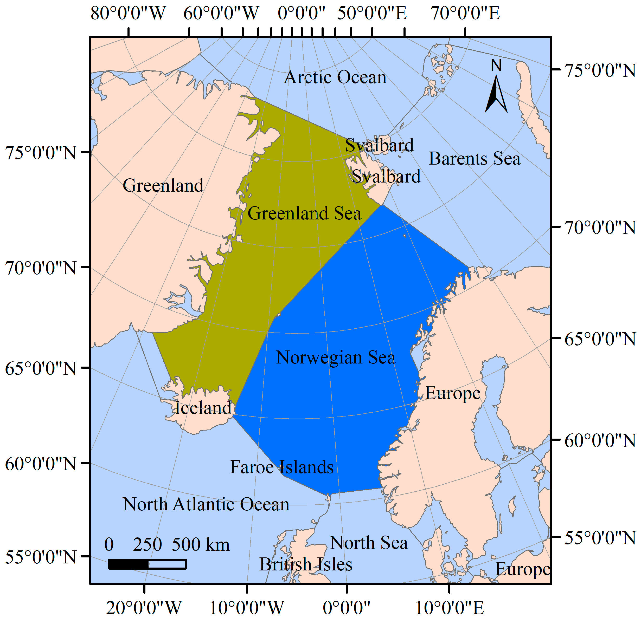
Figure 1. Location of the Greenland Sea and the Norwegian Sea.
Remotesensing 16 02477 g001
Figure 2. Annual mean SST of the Greenland Sea and the Norwegian Sea deviating from the 7-year mean. (a) 2015; (b) 2016; (c) 2017; (d) 2018; (e) 2019; (f) 2020; (g) 2021.
Remotesensing 16 02477 g002
Figure 3. Monthly mean SST of the whole regions of the Greenland Sea and the Norwegian Sea.
Remotesensing 16 02477 g003
Figure 4. Sliding paired t-test with the monthly SST of the two seas. (a) Greenland Sea; (b) Norwegian Sea.
Remotesensing 16 02477 g004
Figure 5. Trends of the monthly mean SST of the two seas and the linear fits. (a) Greenland Sea; (b) Norwegian Sea.
Remotesensing 16 02477 g005
Figure 6. Irregular components of the monthly mean SST of the two seas. (a) Greenland Sea; (b) Norwegian Sea.
Remotesensing 16 02477 g006
Figure 7. Monthly mean atmospheric CO2 concentrations over the Greenland Sea and the Norwegian Sea and the concentration difference between them.
Remotesensing 16 02477 g007
Figure 8. Sliding paired t-test with the monthly mean atmospheric CO2 concentrations over the two seas. (a) Greenland Sea; (b) Norwegian Sea.
Remotesensing 16 02477 g008
Figure 9. Trends of the monthly mean atmospheric CO2 concentrations over the two seas.
Remotesensing 16 02477 g009
Figure 10. Irregular components of the monthly mean CO2 concentrations over the two seas. (a) Greenland Sea; (b) Norwegian Sea.
Remotesensing 16 02477 g010
Figure 11. Wavelet coherence and relative phase relationship of the detrended SST of the Greenland Sea and the Norwegian Sea (white lines are contours with 0.05 significance level; phase difference between the SSTs of the two seas with a 0.05 significance level is indicated by the angle of the arrow).
Remotesensing 16 02477 g011
Figure 12. Wavelet coherence and relative phase relationship of the detrended series of the SST and the atmospheric CO2 concentration for the Greenland Sea (white lines are contours with 0.05 significance level; phase difference of SST over CO2 concentration with a 0.05 significance level is indicated by the angle of the arrow).
Remotesensing 16 02477 g012
Figure 13. Wavelet coherence and relative phase relationship of the detrended series of the SST and the atmospheric CO2 concentration for the Norwegian Sea (white lines are contours with 0.05 significance level; phase difference of SST over CO2 concentration with a 0.05 significance level is indicated by the angle of the arrow).
Remotesensing 16 02477 g013
Figure 14. Average global SST. (a) 1880 to 2020; (b) 2001 to 2008; (c) 2015 to 2020.
Remotesensing 16 02477 g014
Table 1. Coefficients of the linear regression with the temperature trends.
RegionMonthsInterceptR2Adjusted R2
Greenland Sea−0.0097 ***266.97 ***0.1450.132
Norwegian Sea−0.0036 **275.82 ***0.1080.095
*** Significant at p < 0.001, ** significant at p < 0.01.
Table 2. Coefficients of the linear regression with the CO2 concentration trends.
RegionMonthsInterceptR2Adjusted R2
Greenland Sea0.207 ***399.94 ***0.9980.998
Norwegian Sea0.208 ***400.03 ***0.9980.998
*** Significant at p < 0.001.
Disclaimer/Publisher’s Note: The statements, opinions and data contained in all publications are solely those of the individual author(s) and contributor(s) and not of MDPI and/or the editor(s). MDPI and/or the editor(s) disclaim responsibility for any injury to people or property resulting from any ideas, methods, instructions or products referred to in the content.