Abstract
Understanding and accurately predicting stomatal conductance in almond orchards is critical for effective water-management strategies, especially under challenging climatic conditions. In this study, machine-learning (ML) regression models trained on multispectral (MSP) and thermal infrared (TIR) data acquired from unmanned aerial vehicles (UAVs) are used to address this challenge. Through an analysis of spectral indices calculated from UAV-based data and feature-selection methods, this study investigates the predictive performance of three ML models (extra trees, ET; stochastic gradient descent, SGD; and extreme gradient boosting, XGBoost) in predicting stomatal conductance. The results show that the XGBoost model trained with both MSP and TIR data had the best performance (R2 = 0.87) and highlight the importance of integrating surface-temperature information in addition to other spectral indices to improve prediction accuracy, up to 11% more when compared to the use of only MSP data. Key features, such as the green–red vegetation index, chlorophyll red-edge index, and the ratio between canopy temperature and air temperature (Tc-Ta), prove to be relevant features for model performance and highlight their importance for the assessment of water stress dynamics. Furthermore, the implementation of Shapley additive explanations (SHAP) values facilitates the interpretation of model decisions and provides valuable insights into the contributions of the features. This study contributes to the advancement of precision agriculture by providing a novel approach for stomatal conductance prediction in almond orchards, supporting efforts towards sustainable water management in changing environmental conditions.
1. Introduction
Climate change is one of the greatest challenges of the 21st century and has a profound impact on many sectors, especially agriculture. This sector is particularly vulnerable to several climate-related events, such as changes in temperatures, rainfall patterns, and the increased frequency of extreme events like droughts and storms. Such phenomena have a significant impact on agricultural productivity [1,2]. In this context, almond trees, Prunus dulcis (var. dulcis (Rosaceae)), are considerably affected by the negative impacts of climate change, so it is crucial to apply appropriate management practices to ensure their sustainability and productivity [3]. A fundamental aspect of managing agriculture under changing climatic conditions is assessing plant water conditions [4]. Measuring stomatal conductance (gsw) provides an indicator of plant water status. It reflects the degree of stomatal opening, which dynamically adjusts in response to plant stress levels. By monitoring this physiological parameter, farmers can optimize irrigation scheduling, especially during periods of water stress, to ensure efficient water use and crop health [5]. Understanding the relationship between stomatal conductance and environmental factors like temperature, light intensity, atmospheric CO2 concentration, relative humidity, and soil moisture content allows for more sustained management strategies to enhance crop productivity, as it is directly linked to a plant’s ability to regulate water loss through the stomata and, consequently, its water-use efficiency [6]. In the specific case of almond cultivation, the assessment of water stress based on stomatal conductance is crucial for efficient irrigation management and the application of bio-stimulants that can mitigate the effects of stress [7].
The porometer is an efficient and valuable tool for measuring stomatal conductance. However, a significant disadvantage of this type of tool is that only a small number of leaves per tree are measured, potentially missing broader trends across the entire plant or orchard [8]. In contrast, remote-sensing (RS) techniques offer a more comprehensive approach. The major advantage of using RS techniques is that, theoretically, all trees and all leaves contribute to the parameter estimation, providing a more holistic view of plant health and water status. This broader scope is essential for global-scale monitoring and management of agricultural resources, emphasizing the importance of RS for understanding and mitigating the impacts of climate change. Considering the automatic prediction of stomatal conductance based on RS data, namely through the use of spectral indices, Quemada et al. [9] studied the role of RS in tracking crop water stress levels using a range of platforms, such as satellites, manned aerial vehicles, and unmanned aerial vehicles (UAVs). These platforms offer high-resolution imagery and are becoming increasingly accessible, along with sensors such as standard RGB, multispectral (MSP), hyperspectral (HSP), and thermal infrared (TIR). RGB cameras capture spectral ranges within the visible bands [10], while MSP and HSP cameras cover a broader spectrum in the visible–infrared (VIS/IR) frequency range [11]. TIR cameras measure emissions within the 7.5–13.5 μm spectral range. The choice of sensors depends on monitoring goals and available resources. RGB cameras are beneficial for color analysis, whereas MSP and HSP cameras offer a more comprehensive plant analysis [12]. On the other hand, TIR cameras are especially valuable for monitoring drought stress by measuring canopy temperature and estimating transpiration rates [13,14].
Considering general studies using RS data to predict stomatal conductance, Bian et al. [15] developed a simplified approach for monitoring cotton water stress using UAV-based MSP and TIR imagery. The proposed method uses the crop water stress index (CWSI) [16] calculated from canopy temperature data. The results showed that the simplified CWSI (CWSIsi) was more accurate and had a higher sensitivity to cotton water stress changes compared to other empirical methods, such as empirical CWSI (CWSIe). The study also shows a strong correlation between the CWSIsi and the physiological parameters of cotton, including stomatal conductance and soil moisture content. Sobejano-Paz et al. [17] used HSP and TIR imagery, mounted on a UAV, to estimate the stomatal conductance and physiological parameters in maize and soybean plants under different water regimes. Several indices were computed that were related to vegetation status, water stress, and stomatal conductance. The models that were developed had high accuracy in estimating stomatal conductance, with coefficients of determination (R2) ranging from 0.73 to 0.93, highlighting the potential of HSP and TIR for plant physiological monitoring. On the other hand, Xie et al. [18] used an MSP sensor to collect data on the different stages of growth and development of citrus trees. Several models were applied in the prediction of citrus stomatal conductance, including support vector regression (SVR), random forest (RF), and k-nearest neighbor (kNN).
Regarding stomatal conductance prediction in almond orchards, several studies used RS data. Camino et al. [19] investigated the spatial variability of the CWSI within almond-tree canopies and its effects on the relationship with stomatal conductance. Their study was conducted in an almond orchard cultivated under three irrigation regimes using high-resolution (25 cm) TIR imagery acquired by aircraft. Different automatic object-based tree-crown detection algorithms based on temperature quartile thresholds were employed for image segmentation. The results showed a strong linear inverse relationship between CWSI and stomatal conductance across all thermal classes. However, the strength of this relationship was significantly affected by the crown segmentation strategy. Moreover, the relationship with stomatal conductance improved when CWSI values corresponded to the coldest and purest vegetation pixels (R2 = 0.78 from pure vegetation pixels vs. R2 = 0.52 when using warmer pixels). Gutiérrez-Gordillo et al. [20] aimed to monitor the emerging water stress on almond trees under irrigated and regulated deficit irrigation treatments. Stem water potential, net photosynthetic rate, and stomatal conductance were monitored in the field, while NDVI and CWSI were computed using MSP and TIR images acquired by UAV. The results showed that the NDVI and CWSI can be used as reliable indicators of plant water status and as substitutes for stomatal conductance, particularly under mild water stress conditions. García-Tejero et al. [21] studied the efficiency of thermography as a non-invasive technique for monitoring the water status of almond trees subjected to various irrigation regimes. The authors aimed to identify the optimal time of day for acquiring TIR data and the most reliable thermal index for interpreting crop water stress. The results revealed a statistically significant correlation between thermal indices and stomatal conductance. Specifically, the CWSI showed a strong correlation with stomatal conductance, with values ranging from −0.86 to −0.98 across the different evaluation times.
Despite the established correlations between each index derived from the RS data and stomatal conductance in almond orchards, these relationships often fail to capture the intricate interplay of several features influencing stomatal dynamics. This limitation highlights the need for more sophisticated approaches, such as machine-learning (ML) models, to accurately predict stomatal conductance, particularly in almond orchards where such research is currently lacking. In this study, this gap is addressed by employing different ML regression models to predict stomatal conductance in an almond orchard. Using MSP and TIR UAV-based data to compute different indices. These spectral indices serve as features for the ML models. To further capture the complex relationships between spectral indices and stomatal conductance, the Shapley additive explanations (SHAP) values were explored to provide a unique perspective on the contribution of each individual feature to the model predictions.
2. Materials and Methods
2.1. Study Area
The study was conducted on two dates (14 July and 28 August 2023) in a rain-fed almond orchard in São Salvador (41°25′55″N, 7°08′06″W; Figure 1a), Mirandela, Trás-os-Montes region in Northeastern Portugal. Almond cultivation has a long tradition in this region, and the almond trees play an important role in the region’s economy and cultural identity. The abundance of almond trees in this region contributes to its picturesque landscapes and supports the production of high-quality almonds [22].
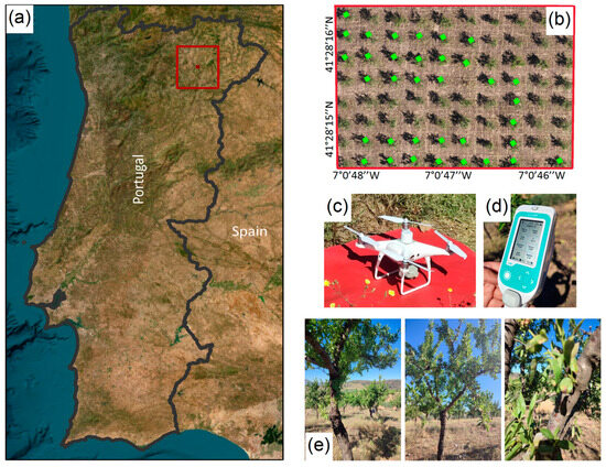
Figure 1.
Overview of the almond orchard under study: (a) location of the study area; (b) identification of almond trees used in data collection in the studied orchard; (c) P4 multispectral multirotor unmanned aerial vehicle; (d) LI-600 porometer/fluorometer used in data collection; and (e) perspectives of rain-fed almond trees.
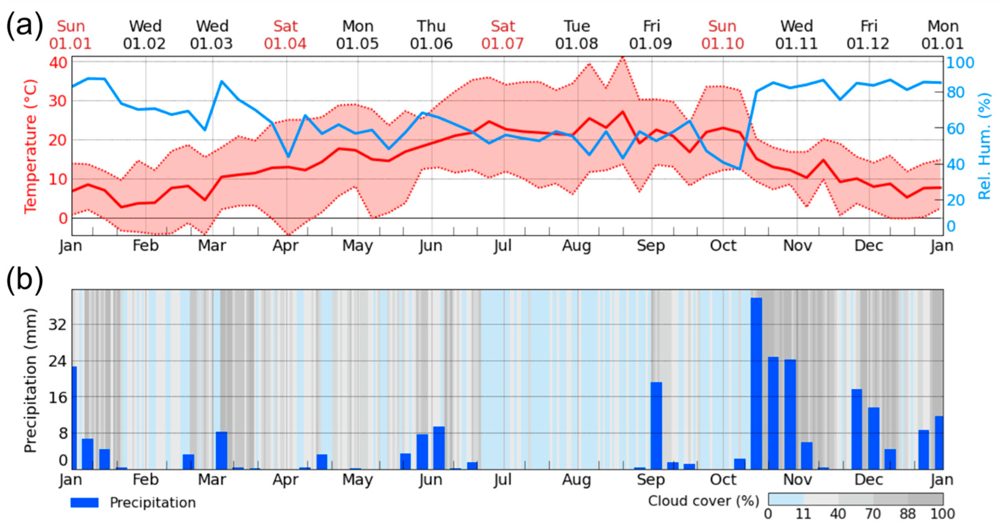
Trás-os-Montes has a Mediterranean climate with hot, dry summers and cold, harsh winters, which are suitable for almond cultivation. High temperatures and low rainfall during the growing season promote the optimal development and ripening of almond trees (Figure 2a,b), making Trás-os-Montes a prime location for almond production [23]. The data for this study was collected in July and August 2023. Figure 2a,b illustrate the lack of rainfall and the increase in temperatures during these summer months, which contributed to increased stress levels in the almond trees.
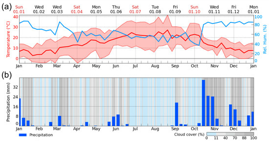
Figure 2.
Weather conditions of 2023 in Mirandela: (a) air temperature and humidity values and (b) rainfall values. Data from Meteoblue.
2.2. Data Collection and Processing
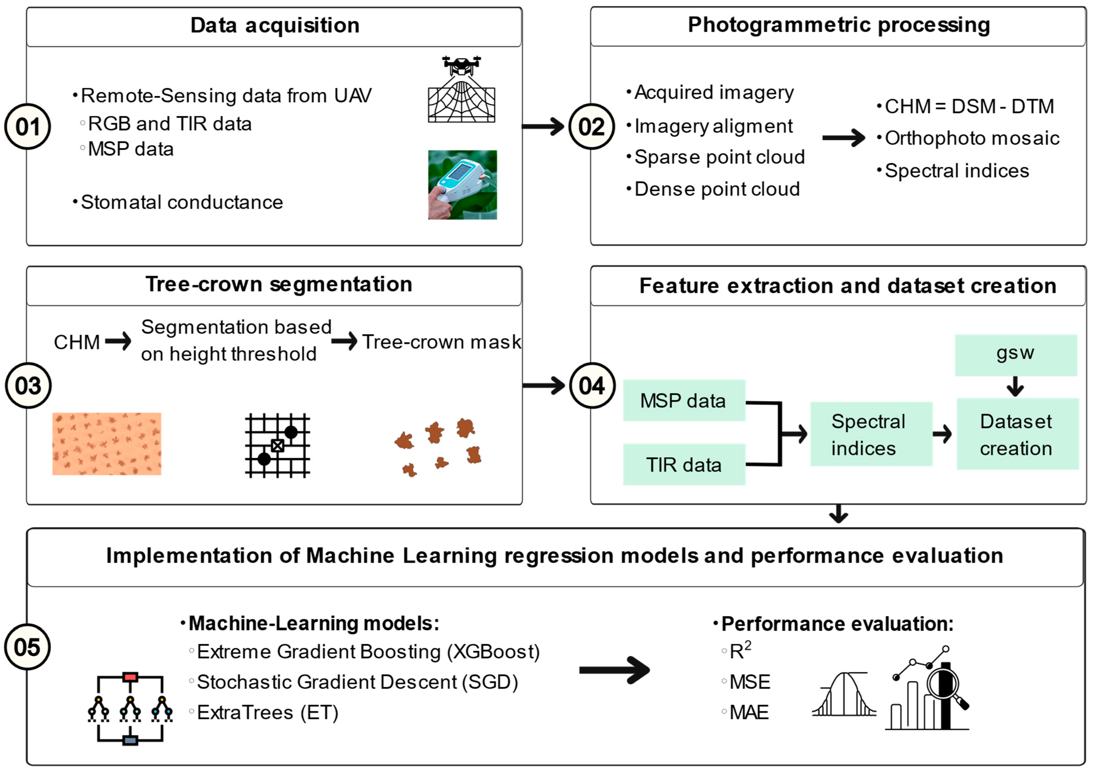
The development of the study involved several steps (Figure 3). In the first step, data acquisition, the RGB and TIR data were collected using two UAVs, and the stomatal conductance data were acquired using a porometer. In the second step, the acquired UAV data were processed to obtain orthorectified raster products. Subsequently, in the third step, the tree-crown segmentation was performed. In the fourth step, the features were extracted for each tree, and a dataset was created. In the fifth and final step, ML regression models were implemented, and their performance was evaluated.
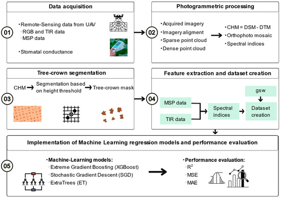
Figure 3.
Data collection and processing workflow: (1) data acquisition; (2) photogrammetric processing; (3) tree-crown segmentation; (4) feature extraction and dataset creation; (5) implementation of machine-learning regression models and performance evaluation.
2.2.1. UAV Data Collection
The MSP data used for this study were acquired with the P4 Multispectral multi-rotor UAV (DJI, Shenzhen, China). It is equipped with six 1/2.9-inch CMOS sensors (2.08-megapixel resolution), one RGB sensor (not used in this study), and five monochrome sensors that can capture data in blue (450 nm ± 16 nm), green (560 nm ± 16 nm), red (650 nm ± 16 nm), red edge (730 nm ± 16 nm), and near infrared (840 nm ± 26 nm). In turn, the RGB and TIR data were captured using a Mavic 3T multi-rotor UAV (DJI, Shenzhen, China). This UAV is equipped with an RGB camera (1/2-inch CMOS sensor, 12-megapixel resolution) and a thermal imaging sensor (640 × 512 pixels, 8–14 μm wavelength range, uncooled VOx microbolometer, CA, USA). All sensors are integrated into a 3-axis gimbal for image stabilization. Both UAVs are equipped with an RTK module, which ensures high accuracy in georeferencing the images.
The data acquisition was carried out on two dates. On 14 July 2023, the flight mission to collect MSP data was carried out at a flight height of 60 m, a UAV speed of 2.3 m/s, and an image overlap of 80% in the longitudinal direction and 70% in the transverse direction. The number of images taken was 1390, which corresponds to 278 different captures (five images per capture). The area covered by the UAV flight was 4.75 ha with a spatial resolution of 3.13 cm. The flights to collect the TIR and RGB data were conducted on the same day and at a flight height of 60 m, with a flight speed of 4 m/s, a longitudinal image overlap of 90%, a lateral image overlap of 70%, and captured 656 images. The area covered by the UAV flight was approximately 7 ha, with a spatial resolution of 7.68 cm for the TIR images and a spatial resolution of 1.91 cm for the RGB images. On 28 August 2023, the flights were conducted under the same conditions as the previous flights. During the MSP data acquisition, 1455 images were captured, which corresponds to 291 different captures (five images per capture). The area covered by the UAV flight was 5.45 ha, which corresponds to a spatial resolution of 3.53 cm. During the flight mission to collect the TIR and RGB data, 750 images were captured. The area covered by the UAV flight was approximately 7 ha, with a spatial resolution of 7.64 cm for the TIR images and a spatial resolution of 1.89 cm for the RGB images.
Regarding real-time kinematic (RTK) corrections, these were maintained via a connection to the Portuguese Network of GNSS Permanent Stations (ReNEP), which was linked to a nearby station, approximately 10 km from the study area, in the city of Mirandela. ReNEP collects data from GPS, GLONASS, GALILEO, and BEIDOU satellite navigation systems. This enabled the achievement of horizontal and vertical accuracies below 0.02 m and 0.04 m, respectively, for UAV-based imagery through real-time correction data. This precision was deemed adequate for our study. To ensure coverage during data collection, a hotspot was established using an Android smartphone, connecting the UAV remote controllers.
2.2.2. Stomatal Conductance Acquisition
Stomatal conductance data (mol m−2 s−1) were collected in the studied almond orchard using the LI-600 Porometer/Fluorometer (LI-COR, Lincoln, NE, USA) in automatic mode (auto-mode option), between 10:00 am and 11:00 am. Stomatal conductance data collection was conducted during the UAV flight campaigns on 14 July (35 trees) and 28 August (35 trees), 2023. In each campaign, we measured 35 trees and collected stomatal conductance measurements from 10 expanded leaves per tree. These leaves were randomly selected from different parts of the canopy with direct sun exposure and without shadows in front of the sensor to not affect ambient light-level readings. This approach ensured representative sampling by selecting leaves randomly from different parts of the canopy. In this way, it is possible to capture intra-tree variability and ensure a robust representation of each tree’s stomatal conductance. This methodology helps account for the potential variability in stomatal conductance within individual trees and provides a more comprehensive dataset for correlation analyses.
The LI-600 Porometer/Fluorometer (LI-COR, Lincoln, NE, USA) is a compact, handheld instrument that combines porometry and fluorometry. This allows for a rapid assessment of stomatal conductance and chlorophyll a fluorescence, which were not considered for this study. The porometer uses a mass balance to calculate stomatal conductance based on water-vapor flux from the leaf, while the fluorometer employs optical techniques to directly measure chlorophyll a fluorescence. Offering versatility, the LI-600 can function as either a dedicated porometer or fluorometer, delivering accurate and high-throughput measurements on the same leaf area [24].
2.2.3. Photogrammetric Processing and Spectral Indices Computation
MSP, RGB, and TIR data acquired from the UAV platform were subjected to a photogrammetric workflow through Pix4DMapper Pro (Pix4D SA—version 4.9.0, Lausanne, Switzerland). This software applies structure from motion (SfM) algorithms to reconstruct the three-dimensional (3D) structure of the scene from the captured imagery, generating point clouds from common points between the images. The interpolation of dense point clouds allows for the generation of several orthorectified raster outputs, including digital surface models (DSMs), digital terrain models (DTMs), orthophoto mosaics (derived from the RGB data), and spectral indices. The CHM was derived from the DSM and DTM through a subsequent processing step in QGIS.
The different spectral indices generated during the photogrammetric processing of the MSP and TIR imagery are presented in Table 1. These indices were subsequently considered in the dataset creation process. For the CWSI computation, Twet was determined by spraying leaves with water to simulate full transpiration, and leaf temperature was recorded using an infrared thermometer. To obtain Tdry, leaves with direct solar incidence were covered with petroleum jelly to prevent transpiration. Temperature readings were obtained 15 min after this procedure. Additionally, the air temperature (Ta) was collected using a humidity and temperature data logger (SSN-22, Hairuis Instruments, Shenzhen, China).

Table 1.
List of spectral indices used in dataset creation and their respective equations. MSP: multispectral; TIR: thermal infrared; B: blue; G: green; R: red; RE: red edge; N: near infrared; T: temperature.
2.2.4. Tree-Crown Segmentation, Feature Extraction, and Dataset Creation
The segmentation of individual tree crowns was achieved using the CHM. During this step, a threshold of 0.5 m was used to remove soil and other low vegetation. This process resulted in a binary mask, which was then vectorized to generate a set of polygons representing each identified tree crown. Following this, the mean value of the computed spectral indices was associated with each tree-crown polygon using the QGIS “Raster Statistics for Polygons” tool. The resulting data were transformed into the dataset used in this study with 22 features. These features correspond to the indices obtained from the MSP data (BNDVI, CCCI, CIRE, GBNDVI, GBVI, GN, GNDVI, GRNDVI, GRVI, NDRE, NDVI, PSRI, RBNDVI, RBVI, REn, RN, SRPI and, SIPI), the TIR data (CWSI, Ig, and Tc-Ta), and a target feature representing the stomatal conductance values (gsw). There is a total of 70 samples in the dataset, corresponding to the data extracted from trees on both 14 July and 28 August 2023 (Figure 1b).
2.3. Application of Machine-Learning Regression Models
The application of ML regression models (fifth step of Figure 3) included four main procedures: feature selection, model implementation, hyperparameter tuning, and model evaluation.
2.3.1. Feature-Selection Process
The selection of features is a crucial step in the process of ML, as it helps in identifying the most informative features within the generated dataset. This process can impact the performance of the regression models by preventing overfitting, reducing training time, and improving generalization [40]. There are different methods for feature selection. In this study, Pearson’s correlation, mutual information, and feature importance were considered in the feature-selection process. Pearson correlation helps in the identification of features that are highly correlated with the target feature, while they are only minimally correlated with each other. By selecting features that are highly correlated with the target feature, we can reduce the dimensionality of the dataset and improve model performance [41]. On the other hand, mutual information is a measure of the amount of information a feature provides about the target. It assists in the selection of features based on their mutual information with the target variable. By selecting features with high mutual information, it is possible to identify the features that are most informative and relevant for predicting the target variable [42]. However, both methods may not be the best options to capture complex and non-linear relationships between features and the target variable. Therefore, it is important to consider other options such as feature importance, which is a method that involves assigning a score or weight based on its importance in the model. This can be done using techniques such as permutation feature importance or the feature importance of a tree-based model. By identifying the features that are most important to the model, it is possible to reduce the dimensionality of the dataset and improve the performance of the models [43,44].
2.3.2. Selection and Implementation of Machine-Learning Regression Models
For the prediction of stomatal conductance, three different regression models were considered, which have proven successful for similar research problems: extra trees (ET), stochastic gradient descent (SGD), and extreme gradient boosting (XGBoost). ET is a tree-based ensemble method for supervised learning that can be used for both classification and regression tasks. It works by constructing many unpruned decision trees on random sub-samples of the training dataset and outputting the average (for regression) or majority class prediction. ET has several advantages over other ensemble methods, such as random forest (RF) and tree bagging (TB), including faster computation times, no requirement for pre-sorting of the training data, and improved accuracy on certain datasets. It is particularly useful for large and high-dimensional datasets where computational complexity is a concern. This method can also handle noisy or missing data and requires minimal parameter tuning. Overall, ET is a highly promising method for supervised learning that offers excellent performance and scalability in a wide range of applications [45]. The SGD is a popular optimization algorithm that excels in handling large-scale ML problems and overcoming computational and memory constraints. It iteratively updates a function’s weights using small, randomly sampled portions of the training data rather than the entire dataset. Additionally, SGD can handle functions with discontinuities and can be easily distributed across multiple computing nodes. Overall, SGD offers a flexible and scalable approach to optimization, contributing to its widespread adoption in ML applications [46]. XGBoost is an ML technique that achieves similar prediction accuracy to RF while offering greater user friendliness. This is due to XGBoost having fewer hyperparameters requiring tuning. Moreover, XGBoost leverages an “additive strategy” that builds upon the foundations of gradient boosting. It aims to minimize a regularized objective function by employing several techniques. These include penalizing model complexity, smoothing the final learned weights to prevent overfitting, and reducing the influence of individual trees through column subsampling and shrinkage. Additionally, it incorporates a sparsity-aware split-finding approach, allowing for efficient training on sparse datasets [47].
For the implementation of ML regression models, we employed a cross-validation (CV) technique, splitting the dataset into five training and testing sets. To augment the size of the training sets and improve model generalizability, we further incorporated the bootstrap method. It works by creating multiple new datasets, each containing samples drawn with replacements from the original data. This process injects diversity into the training process, leading to several benefits. Bootstrapping can help in reducing overfitting, improving the robustness of models to unseen data, and providing a more reliable estimate of a model’s generalizability [48]. With this method, the original training dataset, which consisted of 57 samples (out of the total 70 samples), suffered a 10-fold increase.
2.3.3. Hyperparameter Tuning
Hyperparameters are parameters that are not learned from the data but are defined before the learning process begins. The choice of hyperparameters can have a significant impact on the performance of the model, so tuning the hyperparameters is an important step in the ML pipeline. There are various techniques for tuning hyperparameters, including grid search, random search, and Bayesian optimization. Grid search tests all possible combinations of hyperparameters within a predefined range. In this study, the GridSearchCV was the method applied to test the best hyperparameters for each applied model.
Regardless of using only MSP features and the combination of MSP and TIR features, the defined hyperparameters for ET (max_depth: None; n_estimators: 50), SGD (learning_rate: adaptive; max_iter: 100,000), and XGBoost (max_depth: 3; n_estimators: 100) were the same.
2.3.4. Model Evaluation and Feature Contributions
Several metrics were employed to assess the performances of the regression models. These included the coefficient of determination (R2), the mean squared error (MSE), and the mean absolute error (MAE). R2 quantifies the proportion of variance in the dependent variable that can be explained by the independent variables in the regression model. The MSE considers the average squared difference between the observed and predicted values. Meanwhile, in contrast, MAE is calculated as the average of the absolute differences between the predicted and observed values of the dependent variable. MAE measures the average magnitude of errors made by the model in the same units as the dependent variable [49].
Feature contributions to model output were assessed using Shapley additive explanations (SHAP), which is a method for explaining the predictions of ML models. SHAP values are a game-theoretic approach to explain the output of any model for any instance. They are based on the concept of cooperative game theory and are inspired by the Shapley value, which is a solution concept in cooperative game theory [50].
3. Results
3.1. Stomatal Conductance Variability
The stomatal conductance measurements taken on 14 July and 28 August 2023 showed contrasts (Figure 4). Stomatal conductance is a sensitive indicator of plant water status, and its values tend to be higher when plants are under low water stress and lower when they are under high water stress [51]. On 14 July, stomatal conductance values were higher, indicating that the almond trees were under less water stress at that time. This could be due to the availability of higher soil moisture and favorable weather conditions, such as cooler temperatures and higher humidity, which may reduce the evaporative demand and, thus, the water stress of the trees [51]. In contrast, stomatal conductance values were lower on 28 August, suggesting that the almond trees were exposed to higher water stress. This could be due to a combination of factors, such as a decrease in soil moisture due to the lack of rainfall or a high evaporative demand due to the hot and dry weather conditions [52], as demonstrated in Figure 2. Reduced stomatal conductance is a survival mechanism that plants use to conserve water and reduce transpiration, which can help them handle water stress [53].

Figure 4.
Observations of stomatal conductance (gsw) per tree (a) and (b) distribution of stomatal conductance (gsw) measured on 14 July and 28 August 2023.
3.2. Feature Analysis, Correlation Assessment, and Feature Selection
Implementing the feature importance methods, during ML model development, resulted in the selection of the six most important features for both scenarios: using only MSP imagery and using both MSP and TIR imagery. The selected fea-tures varied across models. When using only features derived from MSP data, features like GRVI, SRPI, RN, NDVI, RBVI, and SIPI were considered for ET, while for SGD the features with more importance were CIRE, SRPI, GRVI, REn, CCCI, and RBVI. In the XGBoost the top six features were RBNDVI, GRVI, RN, GBNDVI, CIRE, and GNDVI. When features from TIR data are included the feature importance changes for all models, with GRVI, Tc-Ta, RN, SRPI, RBVI, and SIPI having the highest feature importance in ET. While for SGD and XGBoost the features with higher importance were Tc-Ta, REn, CWSI, CIRE, Ig, SRPI and Tc-Ta, RBNDVI, GBNDVI, GNDVI, RBVI, CIRE, respectively.
When analyzing the features derived solely from MSP imagery, the evaluated ML approaches exhibited a preference for features with high linear correlation to the target variable and high mutual information values (Figure 5a,b). Examples include CIRE, GRVI, and SRPI. Interestingly, some models, like SGD, also selected features with lower correlation and mutual information, such as the spectral index REN. Expanding the feature set to include both MSP and TIR data, Tc-Ta (the ratio between canopy temperature and air temperature), CIRE, GRVI, and RBVI emerged as prominent features across the ML approaches due to their strong correlation with the target variable. However, similar to the MSP-only scenario, SGD again selected features with lower correlation, including REn, CWSI, and Ig. These observations highlight the importance of employing diverse feature-selection methods beyond simple correlation or mutual information analysis. ML models, with their ability to capture intricate and complex feature interactions, can leverage such seemingly less prominent features to achieve more accurate and robust predictions.
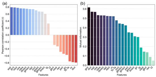
Figure 5.
Correlation between features and the target variable: stomatal conductance (gsw) (a) and mutual information between features and the target variable (b).
3.3. Comparative Evaluation of the Performance of Regression Models in Predicting Stomatal Conductance
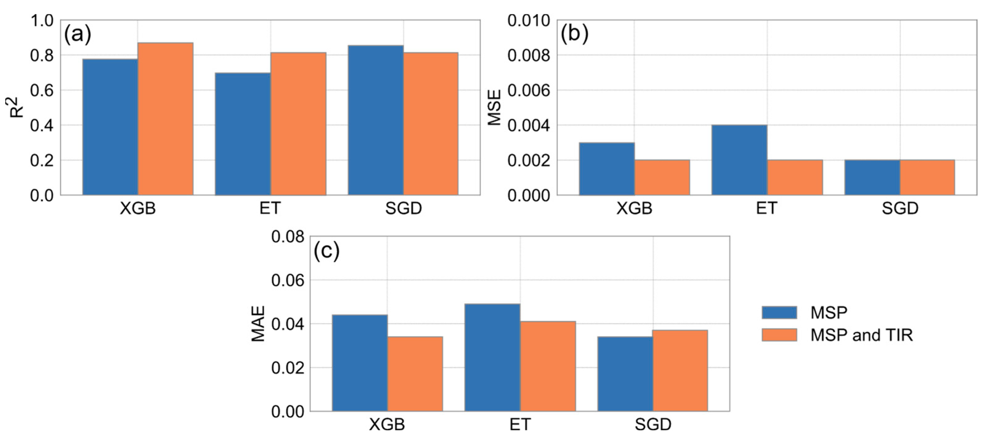
The performance of the implemented ML regression models was evaluated according to the type of features used, more specifically the performance using only MSP data or MSP data in combination with TIR data. By combining ther MSP and TIR data, it was possible to achieve better performance with the XGBoost (XGB) and ET models. On the other hand, the performance of the SGD model was slightly better when only the MSP data was used (Figure 6). When comparing the results according to the model used, it can be observed that the XGBoost model performed the best when using MSP and TIR data, with an R2 of 0.87, an MSE of 0.0016 mol m−2 s−1, and an MAE of 0.035 mol m−2 s−1. Using the XGBoost model with MSP data features resulted in an R2 of 0.78, an MSE of 0.0028 mol m−2 s−1, and an MAE of 0.044 mol m−2 s−1. As for the ET model, the best performance was obtained when using MSP and TIR data, with an R2 of 0.81, an MSE of 0.0023 mol m−2 s−1, and an MAE of 0.041 mol m−2 s−1. When using the ET model with only MSP data, the R2 was 0.70, the MSE was 0.0037 mol m−2 s−1, and the MAE was 0.049 mol m−2 s−1. When using the SGD model, the best performance, although with a slight difference, was obtained with the MSP data, with an R2 of 0.85, an MSE of 0.0018 mol m−2 s−1, and an MAE of 0.034 mol m−2 s−1. When using the SGD model with MSP and TIR data, the R2 was 0.81, the MSE was 0.0023 mol m−2 s−1, and the MAE was 0.037 mol m−2 s−1 (Figure 6).
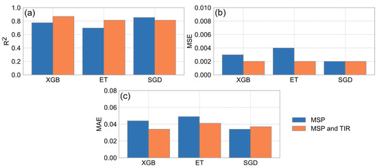
Figure 6.
Performance of regression models in predicting stomatal conductance (gsw). (a) Coefficients of determination (R2), (b) mean squared error (MSE), and (c) mean absolute error (MAE).
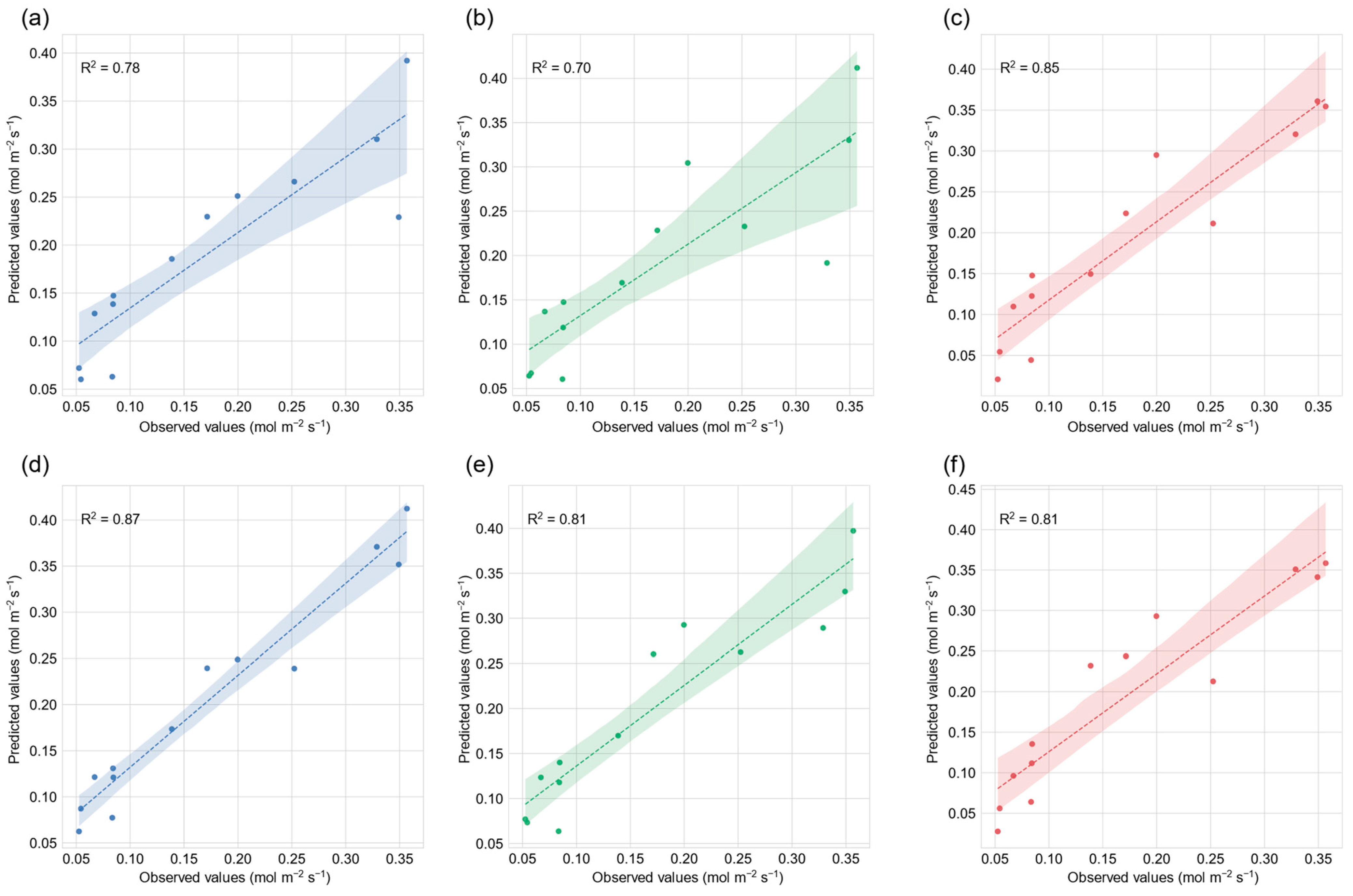
In line with the results of the metrics, the analysis of the scatter plots (Figure 7) shows that models containing both MSP and TIR data (Figure 7d–f) have a higher degree of agreement between the observed and predicted values than models using only MSP data (Figure 7a–c). This is more evident in the XGBoost model (Figure 7d), which shows the most pronounced alignment between the observed and predicted values. On the other hand, the ET model, when based solely on MSP data (Figure 7b), shows the greatest deviation between the observed and predicted values.
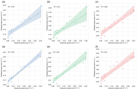
Figure 7.
Scatter plots with observed values and predicted values in the trained models when using multispectral (MSP) data for (a) extreme gradient boosting (XGBoost), (b) extra trees (ET), and (c) stochastic gradient descent (SGD); and when using MSP and thermal infrared (TIR) data for (d) XBoost; (e) ET, and (f) SGD.
3.4. Feature Contributions through Shapley Additive Explanations—SHAP Values
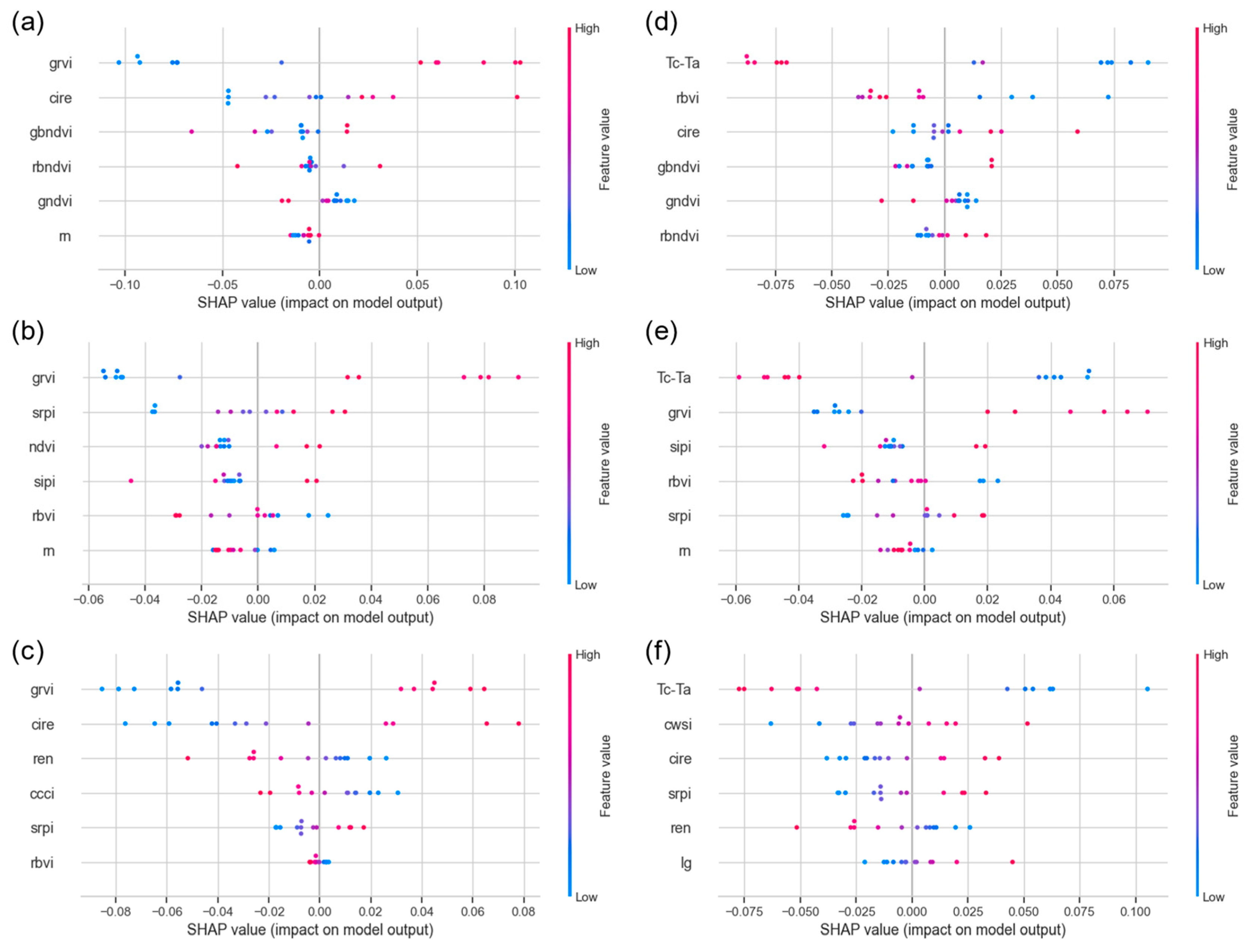
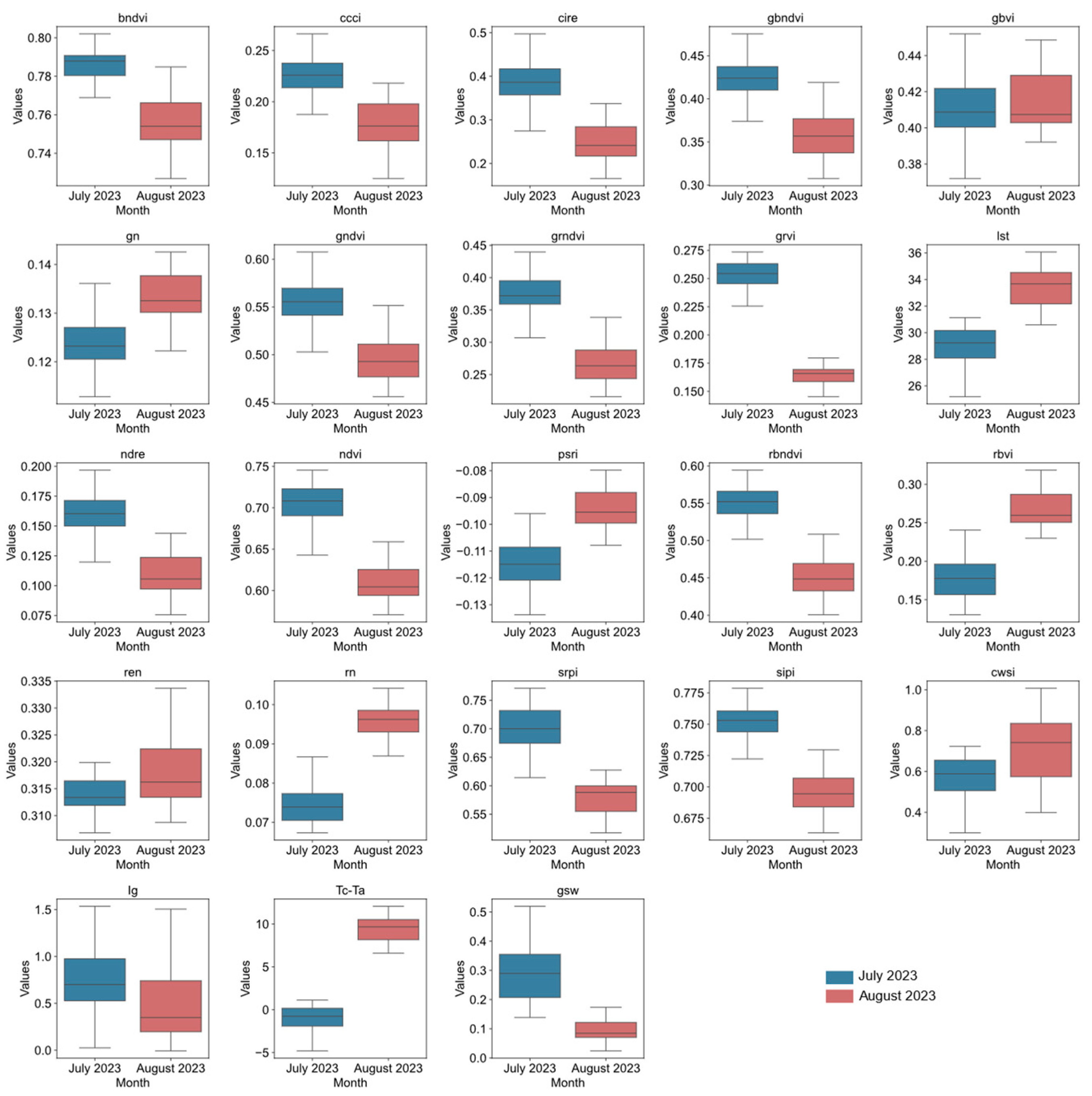
Regarding the SHAP values associated with the selected features for each ML model, it can be observed that, in the MSP data (Figure 8a–c), the feature corresponding to the GRVI index was considered the most important. Higher values of GRVI contributed positively to the prediction of higher values of stomatal conductance, while lower values of GRVI contributed positively to the prediction of lower values of stomatal conductance. These SHAP values are consistent with the results of the Pearson correlations (Figure 5a), as there is a strong positive correlation between GRVI and stomatal conductance. When looking at Figure A1, which shows boxplots of data distribution by data-collection dates, it is also noticeable that the highest GRVI and stomatal conductance values correspond to the data collected on 14 July 2023. Another salient feature is the CIRE using the MSP data in the XGBoost and SGD models (Figure 8a,c), as higher values of this feature also contribute positively to predicting higher values of stomatal conductance.
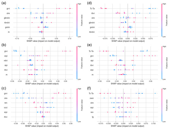
Figure 8.
Shapley additive explanations (SHAP) values for the six most important features when using multispectral (MSP) data for (a) extreme gradient boosting (XGBoost), (b) extra trees (ET), (c) and stochastic gradient descent (SGD) and when using MSP and thermal infrared (TIR) data for (d) XGBoost, (e) ET, and (f) SGD.
Concerning features associated with the use of MSP data in combination with TIR data, the Tc-Ta was found to be the most relevant for the predictions performed. Higher values of this feature significantly contributed to the prediction of lower values of stomatal conductance. These results are also consistent with the correlations between features, as the Tc-Ta shows a strong negative correlation with stomatal conductance. These results are also confirmed by the boxplots (Figure A1), in which the highest values of Tc-Ta were recorded on 28 August 2023, exactly when the lowest values of stomatal conductance were observed.
4. Discussion
In this study, data were collected on two different days, 14 July 2023 and 28 August 2023, using UAV data with RGB, MSP, and TIR sensors, from which several spectral indices were calculated. Stomatal conductance data were also collected on the same days, which showed some contrasts (Figure A1). On 14 July 2023, humidity levels were higher and temperatures were lower than on 28 August 2023, where higher water stress was recorded due to the long absence of rainfall and higher temperatures in August (Figure 2). These differences in the data-collection periods contributed positively to increasing the diversity in the dataset.
Regarding the results obtained, different ML regression models were considered, including ET, SGD, and XGBoost, using features corresponding to MSP indices and a combination of MSP and TIR indices features. For the ET model, the R2 was 0.70 (MSP data) and 0.81 (MSP and TIR data). In the SGD model, the R2 was 0.85 (MSP data) and 0.81 (MSP and TIR data). And for the XGBoost model, the R2 was 0.78 (MSP data) and 0.87 (MSP and TIR data). The highest performance was achieved by the XGBoost model using MSP and TIR data, while the lowest performance was achieved by the ET model using only MSP data. Overall, the models were found to perform better when using a combination of both types of features (MSP and TIR). In relation to other studies related to the use of ML or DL models to predict stomatal conductance, Bagherian et al. [54] attempted to apply ML models using spectral reflectance data for the prediction of stomatal conductance in potato plants. An ensemble ML model and a 1D convolutional neural network (CNN) were used in the study. The results of the study show that both models have the potential to accurately predict stomatal conductance in potato plants. However, the 1D CNN model achieved higher accuracy (R2 = 0.45–0.73) and robustness compared to the ensemble ML model (R2 = 0.44–0.61). Brewer et al. [55] investigated the effectiveness of different models for predicting the stomatal conductance of maize by estimating foliar temperature and stomatal conductance. The researchers obtained the best performance with the RF model (R2 = 0.85). Sobejano-Paz et al. [17] used HSP and TIR imagery, mounted on an UAV, to estimate the stomatal conductance and physiological parameters in maize and soybean plants under different water regimes. Several indices were computed that were related to vegetation status, water stress, and stomatal conductance, including the normalized difference vegetation index (NDVI) [33], transformed chlorophyll absorption in reflectance index (TCARI) [56], pigment-specific normalized difference index (PSNDc) [57], and the photochemical reflectance index (PRI) [58]. The models developed had high accuracy in estimating stomatal conductance, with R2 values ranging from 0.73 to 0.93, highlighting the potential of HSP and TIR for plant physiological monitoring. On the other hand, Xie et al. [18] used an MSP sensor to collect data at different stages of growth and development of citrus trees. The selected optimal index combination for modeling was brightness 808nm (B808), chlorophyll vegetation index (CVI) [59], normalized difference green index (NDGI) [60], and normalized difference red-edge index (NDRE) [32]. The selected indices were used in the predictive models for citrus stomatal conductance, namely in SVR, RF, and kNN. The models performed well with the following R2 and root-mean-square error (RMSE) values: SVR (R2 = 0.9064, RMSE = 0.0043), RF (R2 = 0.8691, RMSE = 0.0050), and KNN (R2 = 0.7677, RMSE = 0.0072).
In the selection process of relevant features for each model, the ‘feature_importance’ function from the scikit-learn library was used. This function evaluates each feature based on its contribution to the model’s predictive accuracy by measuring the decrease in a criterion (e.g., Gini impurity, information gain) when a feature is used to split the data. This method identifies the features with the most significant impact on the model’s performance. Using non-linear models allowed us to capture various linear and non-linear relationships, ensuring that all of the selected features contribute meaningfully to the predictions. Among the selected features, GRVI, CIRE, and Tc-Ta should be highlighted due to their importance in model performance. As for the GRVI, several studies demonstrated its ability to identify water stress levels. For example, Ballester et al. [61] evaluated the feasibility of using spectral indices derived from UAV imagery to monitor the effects of water stress in cotton crops and predict fiber quality. The study aimed to evaluate the performance of the GRVI in monitoring the effects of water stress on cotton and compare it with other widely used indices, such as the NDVI and CWSI. The results showed that the GRVI was sensitive to changes in water status under mild water stress conditions but was affected by the long-term effects of water stress, which limited its use in determining the actual water status of the soil and the crop. As for the CIRE index, the study by Wang et al. [62] focused on using UAVs to monitor crop conditions and diagnose water deficiency in winter wheat. The authors summarized the potential of using vegetation indices, including CIRE, in predicting water stress and stomatal conductance. The results suggest that CIRE performs better in late growth-stage predictions. As for the Tc-Ta, its relevance for predicting the water stress level and stomatal conductance is reflected in the study by Liu et al. [63], who found that the ratio of canopy temperature to air temperature is closely related to stomatal conductance and soil water content and, in particular, is linearly related to CWSI. It can serve as an alternative to CWSI for the assessment of water stress in maize, as it is easy to record and simple to calculate.
The implementation of ML models is a major challenge, as most models function like a black box. Therefore, the implementation of strategies and methods that facilitate the interpretation of the models, as well as the way these models use the dataset features to make a final prediction, is fundamental. In this study, SHAP values were used to address this issue. SHAP values provide a principled approach to quantify the contribution of each feature to the model output, which improves the interpretability of the model and facilitates the identification of the main drivers behind its decisions [64]. Using the SHAP values, it was possible to identify how higher values of the GRVI and CIRE features contributed positively to increasing the predicted values of stomatal conductance and how lower values contributed to decreasing these predictions. It was also possible to see the inverse relationship between the Tc-Ta feature and the prediction of stomatal conductance. With this type of information, the interpretive power increased, providing valuable insight into the decision-making process of the ML models and contributing to the understanding of the topic under study. Moreover, SHAP values provide a measure of feature importance based on their contribution to the model predictions, which is not necessarily reflected in correlation or mutual information analyses. Correlation analyses primarily capture linear relationships, while mutual information measures the dependency between features without considering the direction or linearity of the relationship. In contrast, SHAP values reflect the model decision-making process, capturing both linear and non-linear interactions among the features. Thus, features like CWSI and Ig, although showing low correlation with stomatal conductance, may interact with other features in the model in a non-linear manner, resulting in higher SHAP values.
5. Conclusions
This study investigated the prediction of stomatal conductance in almond orchards using ML regression models trained on MSP and TIR data obtained from UAVs. Key features such as GRVI, CIRE, and Tc-Ta were identified as crucial factors for model performance, emphasizing their relevance for the assessment of water stress and stomatal conductance. The implementation of SHAP values enabled the interpretation of model decisions and improved the understanding of feature contributions. The results show the importance of using different feature-selection methods and integrating both MSP and TIR data for accurate predictions when compared with the use of MSP data only. The XGBoost model using MSP and TIR data showed the best performance, highlighting the importance of including thermal information alongside spectral indices. These results are in line with the findings reported in previous studies that highlight the effectiveness of ML and deep-learning models in predicting stomatal conductance in different crops. However, it is important to note the limitations of this study, including the dataset size. To address this limitation, future work will involve expanding the dataset by extending the data-collection period. This will enable the creation of more comprehensive and diverse training and testing datasets. Considering the ability of RS data to predict the stomatal conductance of almond trees, future work could also focus on the development of integrating these data into a digital twin platform. This platform would be designed to incorporate different types of RS data and Internet of Things (IoT) sensors to monitor complex phenomena, such as water availability, stomatal conductance, and almond tree response in near real time.
Author Contributions
Conceptualization, N.G., J.J.S. and L.P.; methodology, N.G. and L.P.; software, N.G.; validation, N.G.; formal analysis, N.G.; funding acquisition, J.J.S. and P.C.; investigation, N.G., P.C., A.B. and L.P.; resources, J.J.S., P.C. and A.B.; data curation, N.G. and L.P.; writing—original draft preparation, N.G.; writing—review and editing, L.P., J.J.S. and P.C.; visualization, N.G.; supervision, J.J.S., P.C. and A.B. All authors have read and agreed to the published version of the manuscript.
Funding
Financial support was provided by national funds through the FCT—Portuguese Foundation for Science and Technology UI/BD/150727/2020 (https://doi.org/10.54499/UI/BD/150727/2020), under the doctoral program “Agricultural Production Chains—from fork to farm” (PD/00122/2012) and from the European Social Funds and the Regional Operational Programme Norte 2020. This study was also supported by CITAB UIDB/04033/2020 (https://doi.org/10.54499/UIDB/04033/2020), Inov4Agro LA/P/0126/2020 (https://doi.org/10.54499/LA/P/0126/2020), and by CIMO UIDB/00690/2020 (https://doi.org/10.54499/UIDB/00690/2020).
Data Availability Statement
The data that support the findings of this study are available from the corresponding author upon reasonable request.
Conflicts of Interest
The authors declare no conflicts of interest. The funders had no role in the design of the study; in the collection, analyses, or interpretation of data; in the writing of the manuscript; or in the decision to publish the results.
Appendix A

Figure A1.
Boxplots of dataset features (bndvi, ccci, cire, gbndvi, gbvi, gn, gndvi, grndvi, grvi, lst, ndre, ndvi, psri, rbndvi, rbvi, ren, rn, srpi, sipi, cwsi, Ig, Tc-Ta) and target variable (gsw) by collection date.
Figure A1.
Boxplots of dataset features (bndvi, ccci, cire, gbndvi, gbvi, gn, gndvi, grndvi, grvi, lst, ndre, ndvi, psri, rbndvi, rbvi, ren, rn, srpi, sipi, cwsi, Ig, Tc-Ta) and target variable (gsw) by collection date.
References
- Malhi, G.S.; Kaur, M.; Kaushik, P. Impact of Climate Change on Agriculture and Its Mitigation Strategies: A Review. Sustainability 2021, 13, 1318. [Google Scholar] [CrossRef]
- Madrigano, J.; Shih, R.A.; Izenberg, M.; Fischbach, J.R.; Preston, B.L. Science Policy to Advance a Climate Change and Health Research Agenda in the United States. Int. J. Environ. Res. Public Health 2021, 18, 7868. [Google Scholar] [CrossRef] [PubMed]
- Freitas, T.R.; Santos, J.A.; Silva, A.P.; Fraga, H. Reviewing the Adverse Climate Change Impacts and Adaptation Measures on Almond Trees (Prunus dulcis). Agriculture 2023, 13, 1423. [Google Scholar] [CrossRef]
- Fernandes de Oliveira, A.; Mameli, M.G.; De Pau, L.; Satta, D. Almond Tree Adaptation to Water Stress: Differences in Physiological Performance and Yield Responses among Four Cultivar Grown in Mediterranean Environment. Plants 2023, 12, 1131. [Google Scholar] [CrossRef] [PubMed]
- Ellsäßer, F.; Röll, A.; Ahongshangbam, J.; Waite, P.-A.; Hendrayanto; Schuldt, B.; Hölscher, D. Predicting Tree Sap Flux and Stomatal Conductance from Drone-Recorded Surface Temperatures in a Mixed Agroforestry System—A Machine Learning Approach. Remote Sens. 2020, 12, 4070. [Google Scholar] [CrossRef]
- Buckley, T.N.; Mott, K.A. Modelling Stomatal Conductance in Response to Environmental Factors. Plant Cell Environ. 2013, 36, 1691–1699. [Google Scholar] [CrossRef] [PubMed]
- Álvarez-Maldini, C.; Acevedo, M.; Estay, D.; Aros, F.; Dumroese, R.K.; Sandoval, S.; Pinto, M. Examining Physiological, Water Relations, and Hydraulic Vulnerability Traits to Determine Anisohydric and Isohydric Behavior in Almond (Prunus dulcis) Cultivars: Implications for Selecting Agronomic Cultivars under Changing Climate. Front. Plant Sci. 2022, 13, 974050. [Google Scholar] [CrossRef] [PubMed]
- Askari, S.H.; De-Ville, S.; Hathway, E.A.; Stovin, V. Estimating Evapotranspiration from Commonly Occurring Urban Plant Species Using Porometry and Canopy Stomatal Conductance. Water 2021, 13, 2262. [Google Scholar] [CrossRef]
- Quemada, C.; Pérez-Escudero, J.M.; Gonzalo, R.; Ederra, I.; Santesteban, L.G.; Torres, N.; Iriarte, J.C. Remote Sensing for Plant Water Content Monitoring: A Review. Remote Sens. 2021, 13, 2088. [Google Scholar] [CrossRef]
- Xie, C.; Yang, C. A Review on Plant High-Throughput Phenotyping Traits Using UAV-Based Sensors. Comput. Electron. Agric. 2020, 178, 105731. [Google Scholar] [CrossRef]
- Marques, P.; Pádua, L.; Sousa, J.J.; Fernandes-Silva, A. Advancements in Remote Sensing Imagery Applications for Precision Management in Olive Growing: A Systematic Review. Remote Sens. 2024, 16, 1324. [Google Scholar] [CrossRef]
- Jafarbiglu, H. A Comprehensive Review of Remote Sensing Platforms, Sensors, and Applications in Nut Crops. Comput. Electron. Agric. 2022, 23, 106844. [Google Scholar] [CrossRef]
- Ahmad, U.; Alvino, A.; Marino, S. A Review of Crop Water Stress Assessment Using Remote Sensing. Remote Sens. 2021, 13, 4155. [Google Scholar] [CrossRef]
- Cetin, M.; Alsenjar, O.; Aksu, H.; Golpinar, M.S.; Akgul, M.A. Estimation of Crop Water Stress Index and Leaf Area Index Based on Remote Sensing Data. Water Supply 2023, 23, 1390–1404. [Google Scholar] [CrossRef]
- Bian, J.; Zhang, Z.; Chen, J.; Chen, H.; Cui, C.; Li, X.; Chen, S.; Fu, Q. Simplified Evaluation of Cotton Water Stress Using High Resolution Unmanned Aerial Vehicle Thermal Imagery. Remote Sens. 2019, 11, 267. [Google Scholar] [CrossRef]
- Idso, S.B.; Jackson, R.D.; Pinter, P.J.; Reginato, R.J.; Hatfield, J.L. Normalizing the Stress-Degree-Day Parameter for Environmental Variability. Agric. Meteorol. 1981, 24, 45–55. [Google Scholar] [CrossRef]
- Sobejano-Paz, V.; Mikkelsen, T.N.; Baum, A.; Mo, X.; Liu, S.; Köppl, C.J.; Johnson, M.S.; Gulyas, L.; García, M. Hyperspectral and Thermal Sensing of Stomatal Conductance, Transpiration, and Photosynthesis for Soybean and Maize under Drought. Remote Sens. 2020, 12, 3182. [Google Scholar] [CrossRef]
- Xie, J.; Chen, Y.; Yu, Z.; Wang, J.; Li, J. Estimating Stomatal Conductance of Citrus under Water Stress Based on Multispectral Imagery and Machine Learning Methods. Front. Plant Sci. 2023, 14, 1054587. [Google Scholar] [CrossRef] [PubMed]
- Camino, C.; Zarco-Tejada, P.; Gonzalez-Dugo, V. Effects of Heterogeneity within Tree Crowns on Airborne-Quantified SIF and the CWSI as Indicators of Water Stress in the Context of Precision Agriculture. Remote Sens. 2018, 10, 604. [Google Scholar] [CrossRef]
- Gutiérrez-Gordillo, S.; de la Gala González-Santiago, J.; Trigo-Córdoba, E.; Rubio-Casal, A.E.; García-Tejero, I.F.; Egea, G. Monitoring of Emerging Water Stress Situations by Thermal and Vegetation Indices in Different Almond Cultivars. Agronomy 2021, 11, 1419. [Google Scholar] [CrossRef]
- García-Tejero, I.F.; Rubio, A.E.; Viñuela, I.; Hernández, A.; Gutiérrez-Gordillo, S.; Rodríguez-Pleguezuelo, C.R.; Durán-Zuazo, V.H. Thermal Imaging at Plant Level to Assess the Crop-Water Status in Almond Trees (Cv. Guara) under Deficit Irrigation Strategies. Agric. Water Manag. 2018, 208, 176–186. [Google Scholar] [CrossRef]
- Campos, C.R.; Sousa, B.; Silva, J.; Braga, M.; Araújo, S.D.S.; Sales, H.; Pontes, R.; Nunes, J. Positioning Portugal in the Context of World Almond Production and Research. Agriculture 2023, 13, 1716. [Google Scholar] [CrossRef]
- Freitas, T.R.; Santos, J.A.; Silva, A.P.; Fonseca, A.; Fraga, H. Evaluation of Historical and Future Thermal Conditions for Almond Trees in North-Eastern Portugal. Clim. Chang. 2023, 176, 89. [Google Scholar] [CrossRef]
- Haworth, M.; Marino, G.; Atzori, G.; Fabbri, A.; Daccache, A.; Killi, D.; Carli, A.; Montesano, V.; Conte, A.; Balestrini, R.; et al. Plant Physiological Analysis to Overcome Limitations to Plant Phenotyping. Plants 2023, 12, 4015. [Google Scholar] [CrossRef]
- Yang, C.; Everitt, J.H.; Bradford, J.M.; Murden, D. Airborne Hyperspectral Imagery and Yield Monitor Data for Mapping Cotton Yield Variability. Precis. Agric. 2004, 5, 445–461. [Google Scholar] [CrossRef]
- El-Shikha, D.M.; Barnes, E.M.; Clarke, T.R.; Hunsaker, D.J.; Haberland, J.A.; Pinter, P.J., Jr.; Waller, P.M.; Thompson, T.L. Remote Sensing of Cotton Nitrogen Status Using the Canopy Chlorophyll Content Index (CCCI). Trans. ASABE 2008, 51, 73–82. [Google Scholar] [CrossRef]
- Wu, C.; Niu, Z.; Tang, Q.; Huang, W.; Rivard, B.; Feng, J. Remote Estimation of Gross Primary Production in Wheat Using Chlorophyll-Related Vegetation Indices. Agric. For. Meteorol. 2009, 149, 1015–1021. [Google Scholar] [CrossRef]
- Wang, F.; Huang, J.; Tang, Y.; Wang, X. New Vegetation Index and Its Application in Estimating Leaf Area Index of Rice. Rice Sci. 2007, 14, 195–203. [Google Scholar] [CrossRef]
- Pádua, L.; Guimarães, N.; Adão, T.; Marques, P. Classification of an Agrosilvopastoral System Using RGB Imagery from an Un-manned Aerial Vehicle. In EPIA Conference on Artificial Intelligence; Oliveira, P.M., Novais, P., Reis, L., Eds.; Springer: Berlin/Heidelberg, Germany, 2019. [Google Scholar]
- Henriques, H.J.R.; Schwambach, D.A.; Fernandes, V.J.M.; Cortez, J.W. Vegetation indices and their correlation with second-crop corn grain yield in mato grosso do sul, Brazil. Rev. Bras. Milho Sorgo 2021, 20, 13. [Google Scholar] [CrossRef]
- Tucker, C.J. Red and Photographic Infrared Linear Combinations for Monitoring Vegetation. Remote Sens. Environ. 1979, 8, 127–150. [Google Scholar] [CrossRef]
- Thompson, C.N.; Guo, W.; Sharma, B.; Ritchie, G.L. Using Normalized Difference Red Edge Index to Assess Maturity in Cotton. Crop Sci. 2019, 59, 2167–2177. [Google Scholar] [CrossRef]
- Rouse, J.W.; Haas, R.H.; Schell, J.A.; Deering, D.W. Monitoring Vegetation Systems in the Great Plains with ERTS; NASA: Washington, DC, USA, 1974; p. 309.
- Ren, S.; Chen, X.; An, S. Assessing Plant Senescence Reflectance Index-Retrieved Vegetation Phenology and Its Spatiotemporal Response to Climate Change in the Inner Mongolian Grassland. Int. J. Biometeorol. 2017, 61, 601–612. [Google Scholar] [CrossRef]
- Lee, G.; Hwang, J.; Cho, S. A Novel Index to Detect Vegetation in Urban Areas Using UAV-Based Multispectral Images. Appl. Sci. 2021, 11, 3472. [Google Scholar] [CrossRef]
- Guo, Y.; Wang, H.; Wu, Z.; Wang, S.; Sun, H.; Senthilnath, J.; Wang, J.; Robin Bryant, C.; Fu, Y. Modified Red Blue Vegetation Index for Chlorophyll Estimation and Yield Prediction of Maize from Visible Images Captured by UAV. Sensors 2020, 20, 5055. [Google Scholar] [CrossRef] [PubMed]
- Lebourgeois, V.; Bégué, A.; Labbé, S.; Houlès, M.; Martiné, J.F. A Light-Weight Multi-Spectral Aerial Imaging System for Nitrogen Crop Monitoring. Precis. Agric. 2012, 13, 525–541. [Google Scholar] [CrossRef]
- Kureel, N.; Sarup, J.; Matin, S.; Goswami, S.; Kureel, K. Modelling Vegetation Health and Stress Using Hypersepctral Remote Sensing Data. Model. Earth Syst. Environ. 2022, 8, 733–748. [Google Scholar] [CrossRef]
- Jones, H.G. Use of Infrared Thermometry for Estimation of Stomatal Conductance as a Possible Aid to Irrigation Scheduling. Agric. For. Meteorol. 1999, 95, 139–149. [Google Scholar] [CrossRef]
- Pudjihartono, N.; Fadason, T.; Kempa-Liehr, A.W.; O’Sullivan, J.M. A Review of Feature Selection Methods for Machine Learning-Based Disease Risk Prediction. Front. Bioinform. 2022, 2, 927312. [Google Scholar] [CrossRef]
- Jiang, S.; Wang, L. Efficient Feature Selection Based on Correlation Measure between Continuous and Discrete Features. Inf. Process. Lett. 2016, 116, 203–215. [Google Scholar] [CrossRef]
- Salem, O.A.M.; Liu, F.; Chen, Y.-P.P.; Chen, X. Feature Selection and Threshold Method Based on Fuzzy Joint Mutual Information. Int. J. Approx. Reason. 2021, 132, 107–126. [Google Scholar] [CrossRef]
- Guyon, I.; Elisseeff, A. An Introduction to Variable and Feature Selection. J. Mach. Learn. Res. 2003, 3, 1157–1182. [Google Scholar] [CrossRef][Green Version]
- Yahya, A.A.; Osman, A.; Ramli, A.R.; Balola, A. Feature Selection for High Dimensional Data: An Evolutionary Filter Approach. JCS 2011, 7, 800–820. [Google Scholar] [CrossRef]
- Geurts, P.; Ernst, D.; Wehenkel, L. Extremely Randomized Trees. Mach. Learn. 2006, 63, 3–42. [Google Scholar] [CrossRef]
- Bottou, L. Large-Scale Machine Learning with Stochastic Gradient Descent. In Statistical Learning and Data Science; Summa, M.G., Bottou, L., Goldfarb, B., Murtagh, F., Pardoux, C., Touati, M., Eds.; Chapman and Hall/CRC: Boca Raton, FL, USA, 2011; pp. 33–42. ISBN 978-0-429-10768-9. [Google Scholar]
- Sheridan, R.P.; Wang, W.M.; Liaw, A.; Ma, J.; Gifford, E.M. Extreme Gradient Boosting as a Method for Quantitative Structure–Activity Relationships. J. Chem. Inf. Model. 2016, 56, 2353–2360. [Google Scholar] [CrossRef] [PubMed]
- Efron, B.; Tibshirani, R.J. An Introduction to the Bootstrap; Chapman and Hall/CRC: Boca Raton, FL, USA, 1994; ISBN 978-0-429-24659-3. [Google Scholar]
- Tatachar, A.V. Comparative Assessment of Regression Models Based On Model Evaluation Metrics. Int. J. Innov. Technol. Explor. Eng. 2021, 08, 853–860. [Google Scholar]
- Lundberg, S.; Lee, S.-I. A Unified Approach to Interpreting Model Predictions. Adv. Neural Inf. Process. Syst. 2017, 30, 4768–4777. [Google Scholar]
- Jones, H.G. Plants and Microclimate: A Quantitative Approach to Environmental Plant Physiology; Cambridge University Press: Cambridge, MA, USA, 2013; ISBN 978-1-107-51163-7. [Google Scholar]
- Vialet-Chabrand, S.; Lawson, T. Dynamic Leaf Energy Balance: Deriving Stomatal Conductance from Thermal Imaging in a Dynamic Environment. J. Exp. Bot. 2019, 70, 2839–2855. [Google Scholar] [CrossRef]
- Chaves, M.M.; Flexas, J.; Pinheiro, C. Photosynthesis under Drought and Salt Stress: Regulation Mechanisms from Whole Plant to Cell. Ann. Bot. 2009, 103, 551–560. [Google Scholar] [CrossRef] [PubMed]
- Bagherian, K.; Bidese-Puhl, R.; Bao, Y.; Zhang, Q.; Sanz-Saez, A.; Dang, P.M.; Lamb, M.C.; Chen, C. Phenotyping Agronomic and Physiological Traits in Peanut under Mid-Season Drought Stress Using UAV-Based Hyperspectral Imaging and Machine Learning. Plant Phenom. J. 2023, 6, e20081. [Google Scholar] [CrossRef]
- Brewer, K.; Clulow, A.; Sibanda, M.; Gokool, S.; Odindi, J.; Mutanga, O.; Naiken, V.; Chimonyo, V.G.P.; Mabhaudhi, T. Estimation of Maize Foliar Temperature and Stomatal Conductance as Indicators of Water Stress Based on Optical and Thermal Imagery Acquired Using an Unmanned Aerial Vehicle (UAV) Platform. Drones 2022, 6, 169. [Google Scholar] [CrossRef]
- Wu, C.; Niu, Z.; Tang, Q.; Huang, W. Estimating Chlorophyll Content from Hyperspectral Vegetation Indices: Modeling and Validation. Agric. For. Meteorol. 2008, 148, 1230–1241. [Google Scholar] [CrossRef]
- Yang, F.; Dai, H.; Feng, H.; Yang, G.; Li, Z.; Chen, Z. Hyperspectral Estimation of Plant Nitrogen Content Based on Akaike’s Information Criterion. Trans. Chin. Soc. Agric. Eng. 2016, 32, 161–167. [Google Scholar]
- Garbulsky, M.F.; Peñuelas, J.; Gamon, J.; Inoue, Y.; Filella, I. The Photochemical Reflectance Index (PRI) and the Remote Sensing of Leaf, Canopy and Ecosystem Radiation Use Efficiencies: A Review and Meta-Analysis. Remote Sens. Environ. 2011, 115, 281–297. [Google Scholar] [CrossRef]
- Vincini, M.; Frazzi, E.; D’Alessio, P. A Broad-Band Leaf Chlorophyll Vegetation Index at the Canopy Scale. Precis. Agric. 2008, 9, 303–319. [Google Scholar] [CrossRef]
- Nedkov, R. Normalized Differential Greenness Index for Vegetation Dynamics Assessment. Comptes Rendus l’Académie Sci. Vie Sci. 2017, 70, 1143. [Google Scholar]
- Ballester, C.; Brinkhoff, J.; Quayle, W.C.; Hornbuckle, J. Monitoring the Effects of Water Stress in Cotton Using the Green Red Vegetation Index and Red Edge Ratio. Remote Sens. 2019, 11, 873. [Google Scholar] [CrossRef]
- Wang, J.; Lou, Y.; Wang, W.; Liu, S.; Zhang, H.; Hui, X.; Wang, Y.; Yan, H.; Maes, W.H. A Robust Model for Diagnosing Water Stress of Winter Wheat by Combining UAV Multispectral and Thermal Remote Sensing. Agric. Water Manag. 2024, 291, 108616. [Google Scholar] [CrossRef]
- Liu, H.; Gao, Z.; Zhang, L.; Liu, Y. Stomatal Conductivity, Canopy Temperature and Evapotranspiration of Maize (Zea mays L.) to Water Stress in Northeast China. Int. J. Agric. Biol. Eng. 2021, 14, 112–119. [Google Scholar] [CrossRef]
- Hamilton, R.I.; Papadopoulos, P.N. Using SHAP Values and Machine Learning to Understand Trends in the Transient Stability Limit. IEEE Trans. Power Syst. 2024, 39, 1384–1397. [Google Scholar] [CrossRef]
Disclaimer/Publisher’s Note: The statements, opinions and data contained in all publications are solely those of the individual author(s) and contributor(s) and not of MDPI and/or the editor(s). MDPI and/or the editor(s) disclaim responsibility for any injury to people or property resulting from any ideas, methods, instructions or products referred to in the content. |
© 2024 by the authors. Licensee MDPI, Basel, Switzerland. This article is an open access article distributed under the terms and conditions of the Creative Commons Attribution (CC BY) license (https://creativecommons.org/licenses/by/4.0/).


