Article

Mitigating Masked Pixels in a Climate-Critical Ocean Dataset

by
Angelina Agabin
1,
J. Xavier Prochaska
2,3,*,
Peter C. Cornillon
4 and
Christian E. Buckingham
5
1
Applied Math Department, University of California, Santa Cruz, CA 95064, USA
2
Affiliate of the Department of Ocean Sciences, University of California, Santa Cruz, CA 95064, USA
3
Department of Astronomy and Astrophysics, University of California, Santa Cruz, CA 95064, USA
4
Graduate School of Oceanography, University of Rhode Island, Narragansett, RI 02882, USA
5
National Oceanography Centre, Southampton SO14 3ZH, UK
*
Author to whom correspondence should be addressed.
Remote Sens. 2024, 16(13), 2439; https://doi.org/10.3390/rs16132439
Submission received: 1 May 2024 / Revised: 11 June 2024 / Accepted: 12 June 2024 / Published: 3 July 2024

Abstract

:
Clouds and other data artefacts frequently limit the retrieval of key variables from remotely sensed Earth observations. We train a natural language processing (NLP)-inspired algorithm with high-fidelity ocean simulations to accurately reconstruct masked or missing data in sea surface temperature (SST) fields—one of 54 essential climate variables identified by the Global Climate Observing System. We demonstrate that the resulting model, referred to as Enki, repeatedly outperforms previously adopted inpainting techniques by up to an order of magnitude in reconstruction error, while displaying exceptional performance even in circumstances where the majority of pixels are masked. Furthermore, experiments on real infrared sensor data with masked percentages of at least 40% show reconstruction errors of less than the known uncertainty of this sensor (root mean square error (RMSE) 0.1 K). We attribute Enki’s success to the attentive nature of NLP combined with realistic SST model outputs—an approach that could be extended to other remotely sensed variables. This study demonstrates that systems built upon Enki—or other advanced systems like it—may therefore yield the optimal solution to mitigating masked pixels in in climate-critical ocean datasets sampling a rapidly changing Earth.

1. Introduction

One of the most powerful means to assess the fundamental properties of Earth is via remote sensing: satellite-borne observations of its atmosphere, land, and ocean surface. Since the launch of the Television InfraRed Observation Satellite (TIROS) in 1960, the first of the non-military “weather satellites”, remote-sensing satellites have offered daily coverage of the globe to monitor our atmosphere [1]. It was not until the 1970s that our attention was specifically directed at measuring ocean surface properties. Notably, three spacecraft were launched in 1978 that carried sensor payloads for observing in the visible portion of the electromagnetic (EM) spectrum to measure ocean color for biological applications, in the infrared (IR) range to estimate sea surface temperature (SST) and in the microwave band to estimate wind speed, sea surface height and SST [2,3,4,5]. These programs were followed by a large number of internationally launched satellites carrying a broad range of sensors providing improved spatial, temporal and radiometric resolution for terrestrial, oceanographic, meteorological and cryospheric applications [6,7,8].
All satellite-borne sensors observing Earth’s surface or atmosphere sample some portion of the EM spectrum, with the associated EM waves passing through some or all of the atmosphere. The degree to which the signal sampled is affected by the atmosphere is a strong function of the EM wavelength as well as the composition of the atmosphere, with wavelengths from the visible through the thermal infrared (400 nm–15 μ m) being the most affected. This is also the portion of the spectrum used to sample a wide range of surface parameters, such as land use, vegetation, ocean color, SST, snow cover, etc. Retrieval algorithms are designed to compensate for the atmosphere for many of these parameters, but these algorithms fail if the density of particulates, such as dust, liquid or crystalline water (e.g., clouds) is too large. The pixels for which this occurs are generally flagged and ignored. This results in a sparse field, with the masked regions ranging from single pixels to regions covering tens of thousands of pixels in size. On average, for example, only ∼15% of ocean pixels return an acceptable estimate of SST (e.g., [9]).
These gaps represent hurdles in the analysis, especially those requiring complete fields. For example, process-oriented or dynamics-focused research, for which accurate knowledge of the ocean surface is key, suffer tremendously. Moreover, as handling missing data is a common step in most algorithms making use of these data, gap-filling or so-called inpainting techniques introduce errors in the data stream. Finally, even algorithms that properly handle sparse data necessarily bias their results because of the absence of values, e.g., in seasonally, cloud-dominated regions or where other processes hinder accurate measurements. These additional processes might include rain and human-induced radiation in the case of microwave measurements of winds and SST.
To address such data gaps, multiple datasets are often used together with objective analysis interpolation programs to produce what are referred to as Level-4 (L4) products: gap-free fields (e.g., [10,11]). Researchers have also introduced a diversity of algorithms to fill in clouds (see [12] for a review) including methods using interpolation [9], principal component analyses [13,14,15,16], and, most recently, convolutional neural networks [17,18]. For SST, these methods achieve average root mean square errors of ≈0.2–0.5 K and have input requirements ranging from individual images to an extensive time series.
In this manuscript, we introduce an approach, referred to as Enki, similar and independently developed to that recently undertaken by Goh et al. [19], both inspired by the vision transformer masked autoencoder (ViTMAE) model of [20] to reconstruct masked pixels in satellite-derived fields. Guided by the intuition that (1) natural images (e.g., dogs, landscapes) can be described by a language and therefore analyzed with natural language processing (NLP) techniques and (2) one can frequently recover the sentiment of sentences that are missing words and then predict these words, [20] demonstrated the remarkable effectiveness of ViTMAE to reconstruct masked images. This included images with 75% masked data, a remarkable inference. ViTMAE achieves this by splitting an image into patches and tokenizing them. The tokens are processed through a transformer block (encoder) to generate latent vectors. These latent vectors, which represent the model’s understanding of a token’s relationship to other tokens, are then passed through another transformer block (decoder) that reconstructs the image. Central to ViTMAE’s success was its training on a large corpus of unmasked, natural images, and, given the reduced complexity of most remote-sensing data compared to natural images, one may expect even better performance.
We show below that Enki reconstructs images of SST anomalies (SSTa) far more accurately than conventional inpainting algorithms. We demonstrate that the combination of high-fidelity model output and state-of-the-art artificial intelligence produces the unprecedented ability to predict critical missing data for both climate-critical and commercial applications. Furthermore, the methodology allows for the comprehensive estimation of uncertainty and an assessment of systematics. The combined power of NLP algorithms and realistic model outputs represent a significant advance for image reconstruction of remote sensing applications.

2. Methods

The architecture we use for Enki, shown in Figure 1, inputs and outputs a single-channel image, adopts a patch size of 4 × 4 pixels , and uses 256-dimension latent vectors for the embedding and a 512-dimension embedding for the decoder.
Enki works as follows: (1) Images are broken down into 4 × 4 non-overlapping patches. Patches with missing data are masked or, in the case of training, a percentage of patches are randomly masked. The unmasked patches are tokenized, each with a 256-dimensional latent vector, and assigned a positional embedding. (2) The tokens are passed through a standard Transformer encoder, where self-attention is performed to compute a set of attention weights for each latent vector based on its similarity and association to other latent vectors in the image. These latent vectors represent reduced, numerical representations of data that ideally capture the essential characteristics or features of the data. (3) Masked patches are reintroduced, the latent vectors are run through a Transformer decoder, and the full image is reconstructed as 512-dimension latent vectors. (4) A linear projection layer is used to convert the image back to its original size. The final image is created by replacing the unmasked patches of the reconstructed image with the unmasked patches of the original image.
Enki was trained with SST fields from the global, fine-scale ( 1 / 48 ° , 90-level) LLC4320 (Latitude/Longitude-Cap-4320) [21] ocean simulation undertaken as part of the Estimating the Circulation and Climate of the Ocean (ECCO) project. The MIT General Circulation Model (MITgcm) [22,23], on which the LLC4320 is based, is a primitive equation model that integrates the equations of motion on a 1/48° Latitude/Longitude/polar-Cap grid. It is initialized from lower resolution products of the ECCO project and is progressively spun up at higher resolutions. The highest resolution version, LLC4320, is forced at the ocean surface by European Centre for Medium-rangeWeather Forecasting (ECMWF) reanalysis winds, heat fluxes, and precipitation, and at the boundaries by barotropic tides. The approximate one-year simulation (13 September 2011 to 14 November 2012) provides hourly snapshots of model variables, e.g., temperature, salinity and vector currents, at a spatial resolution of ≈1–2 km.
As opposed to using this simulation for training, we could, of course, have used “cloud-free” portions of SST fields obtained from satellite-borne sensors. However, we often find undetected or improperly masked clouds in these fields, which would impact the training of Enki. Furthermore, these fields are geographically biased [9] and would yield a highly imbalanced training set.
The LLC4320 simulations have been widely used in studies investigating submesoscale phenomena [24,25,26], baroclinic tides [27,28], and mission support for the Surface Water and Ocean Topography (SWOT) satellite sensor [29]. As it has a horizontal grid resolution comparable to but slightly coarser than the spatial resolution of most IR satellite SST measurements, and as it is free from fine-scale atmospheric affects, it represents an oceanographic surface approximately equivalent to but reduced in noise relative to IR satellite SST. See [30] for further details about the implementation of atmospheric effects in the LLC4320. Global model-observation comparisons at these fine horizontal scales can also be found in [31,32,33].
Every two weeks beginning on 13 September 2011, we uniformly extracted 2,623,152 “cutouts” of 144 × 144 km 2 from the global ocean at latitudes lower than 57° N, avoiding land. Each of these initial cutouts were re-sized to 64 × 64 pixelcutouts with linear interpolation and mean subtracted. No additional pre-processing was performed.
We constructed a complementary, validation dataset of 655,788 cutouts in a similar fashion. These were drawn from the ocean model on the last day of every 2 months starting 30 September 2011. They were also offset by 0.25 ° in longitude from the spatial locations of the training set.
A primary hyperparameter of the ViTMAE is the training percentage ( t % ); i.e., the percentage of pixels masked during training (currently a fixed value). A value of t % = 30, for example, indicates 30% of the pixels in each training cutout has been randomly masked. While ref. [20] advocates t % = 75 to insure generalization, we generated Enki models with t % = [10,20,35,50,75]. In part, this is because we anticipated applying Enki to images with less than 50% masked data ( m % < 50 ).
For the results presented here, we train using patches with randomly assigned location (and zero overlap). This approach does, however, lead to an inaccurate representation of actual clouds which exhibit spatial correlation on a wide range of scales. Future work will explore how more representative masking affects the results.
Enki was trained on eight NVIDIA-A10 Graphics Processing Unit (GPUs) on the Nautilus computing system. The most expensive t % = 10 model requires 200 h to complete 400 training epochs with a learning rate of l r = 10 4 .
In addition to the LLC4320 validation dataset, we apply Enki to actual remote sensing data. These were extracted from the Level-2 (L2) product of the National Oceanic and Atmospheric Administration (NOAA) processed granules of the Visible-Infrared Imager-Radiometer Suite (VIIRS) sensor [34]. We included data from 2012–2021 and only included 64 × 64 pixel cutouts without any masked data. These data consist of 923,751 cutouts with geographic preference to coastal regions and the equatorial Pacific (see [31]). We caution that while we selected “cloud-free” 64 × 64 pixel regions, we have reason to believe that a portion of these data are, in fact, affected by clouds (e.g., [35]).

3. Results

Figure 2 shows the reconstruction of a representative example from the validation dataset for the Enki model. In this case, the model was trained on cutouts characterized by 20% of the pixels being masked ( t % = 20 model) but applied to a cutout having 30% of its pixels masked ( m % = 30). Aside from patches along the outer edge of the input image, it is difficult to visually differentiate the reconstructed pixels from the surrounding SSTa values. The greatest difference is 0.19 K and the highest root mean square error (RMSE) in a single 4 × 4 pixel patch is 0.07 K with an average RMSE of 0.02 K. As described below, the performance does degrade with higher m % and/or greater image complexity, but to levels generally less than standard sensor error.
In the following sub-sections, we present analyses of Enki performance, first based on synthetic fields, for individual 4 × 4 pixel masks (Section 3.2), mask objects defined as contiguous, non-overlapping 4 × 4 pixel masked regions (Section 3.3), as a function of cutout complexity (Section 3.4), compared with DINEOF (Section 3.5), and compared with bi-harmonic inpainting (Section 3.6) followed by an analysis with satellite-derived SST fields—real data (Section 3.7).

3.1. Bias in Enki

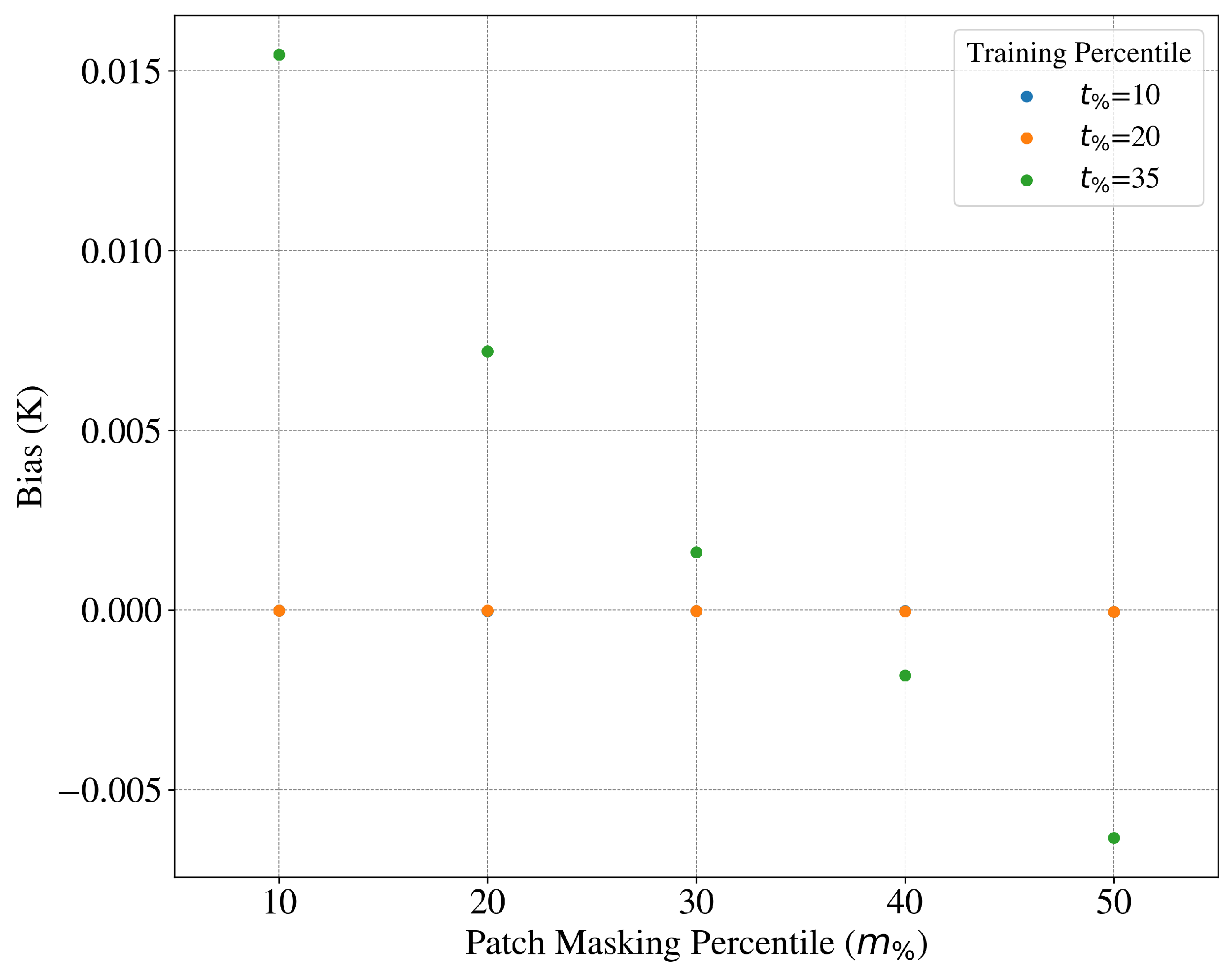
As described in [36], Enki exhibits a systematic bias for cases when m % t % ; i.e., mask fractions significantly lower than the training fraction. Figure 3 describes the magnitude of this bias as a function of t % and m % as derived from the dataset. For the favored model ( t % = 20), the bias term is less than 10 4 K for all m % tested, and can be considered negligible. Indeed, it is at least one order of magnitude smaller than the uncertainty in the average of a 4 × 4 pixel patch in standard IR-based SST retrievals, where the pixel-to-pixel noise is approximately 0.1 K [37]. For all of the results presented here, we have removed the bias calculated from the validation dataset before calculating any other statistic.

3.2. Enki Performance on Individual 4 × 4 pixel Masks—LLC4320 Cutouts

Quantitatively, we consider first the model performance for individual 4 × 4 pixel patches. Figure 4 presents the results of two analyses: (a) the RMSE of reconstruction as a function of the patch spatial location in the image; and (b) the quality of reconstruction as a function of patch complexity, defined by the standard deviation ( σ T ) of the patch in the original image. On the first point, it is evident from Figure 4a that Enki struggles to faithfully reproduce data in patches on the image boundary. This is a natural outcome driven by the absence of data on one or more sides of the patch (i.e., partial extrapolation vs. interpolation). Within this manuscript, we do not include boundary pixels or patches in any quantitative evaluation, and we emphasize that any systems built on a model like Enki should ignore the boundary pixels in the reconstruction.
Figure 4b, meanwhile, demonstrates that Enki reconstructs the data with an RMSE that is over one order of magnitude smaller than that anticipated from random chance. Instead, the results track the relation RMSE ( σ T + 0.014 ) / 9.1 . We speculate that the “floor” in RMSE at σ T < 10 2 K arises because of the loss of information in tokenizing the image patches. The nearly linear relation at larger σ T , however, indicates that the model performance is fractionally invariant with data complexity. We examine these results further in Appendix A.

3.3. Enki Performance on Mask Objects—LLC4320 Cutouts

The above addresses the performance of Enki in the context of individual 4 × 4 pixel squares but two or more of these squares may adjoin one another resulting in larger patches, which we refer to as mask objects. Here, we examine Enki performance as a function of the 23+ million mask objects (for simplicity we will refer to these as masks) extracted from the 655 , 000 cutouts of the validation dataset for t % = 20, m % = 30 . A mask was defined as the union of all 4 × 4 pixel regions, which were touching along a portion of one edge. Two regions with touching corners were not considered to be part of the same mask.
For each mask, its area and minor axis length (the length in pixels of the ellipse with the same normalized second central moment as the region) were determined along with the RMSE of the residual—the difference between SST values of the original field under the mask and the reconstructed field. t % = 20 was selected for consistency with the other analyses presented and m % = 30 to provide for a broad range of mask areas, the larger m % , the more intersections of 4 × 4 pixel masks resulting in larger masks. The median and the log-normalized mean RMSE of the residuals are shown in Figure 5 as a function of (a) mask area and (b) minor axis length. The log-normalized mean is determined by taking the mean of the log of all values falling within a bin and then exponentiating the result. The fact that the log-normalized mean curves (red) and the median curves (black) are very close to the same is an indication that the distribution of the log of the RMSE is close to symmetric about the mean. The vertical gray bars—axis defined on the right hand side of each figure—is a probability histogram of the mask parameter. Because the imposed 4 × 4 pixel mask elements are not permitted to overlap, the area histogram results in 16 pixel steps.
The RMSE of residuals increases linearly with the log10 of the area masked. It is not surprising that the RMSE increases with the area masked; the machine learning (ML) model needs to extrapolate over longer distances. What is surprising is that the rate of increase of the RMSE is so slow, with RMSE increasing from about 0.011 K for a 16 pixel mask to 0.019 K for a 100 pixel mask. The model is performing better than we had anticipated in this regard.
RMSE also increases with the log10 of the minor axis length although more rapidly at first and then more slowly than the dependence on area; i.e., unlike for area, the increase with minor axis length is not linear. The reason we probed the minor axis length is that this length is a measure of how far reconstructed pixels were from available pixels.
Again, in both cases, area and minor axis length, the rate of growth of the RMSE is slow.

3.4. Enki Performance Based on the Complexity of LLC4320 Cutouts

Turning to performance at the full cutout level, Figure 6a shows results as a function of cutout complexity. Here, we examine image complexity versus patch complexity discussed in the context of Figure 4 (Section 3.2) and Figure 5 (Section 3.3). To define cutout complexity, we adopt a deep-learning metric developed by [9] to identify outliers in SSTa imagery. Their algorithm, named Ulmo, calculates a log-likelihood value L L Ulmo designed to assess the probability of a given image occurring within a very large dataset of SST images. Refs. [9,35] demonstrate that data with the lowest L L Ulmo exhibit greater complexity, both in terms of peak-to-peak temperature anomalies and also in terms of the frequency and strength of fronts, etc.
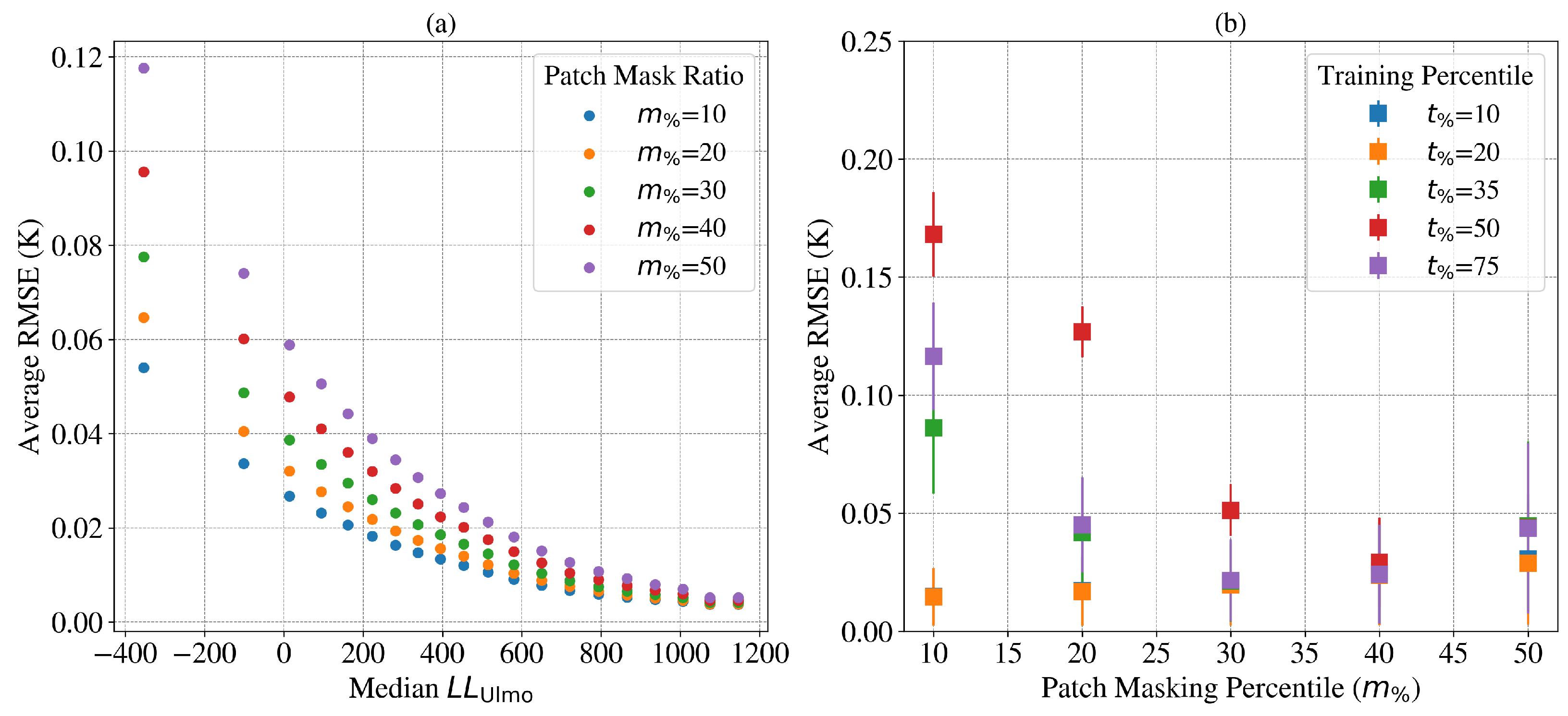
Figure 6a reveals that the reconstruction performance depends on L L Ulmo , with the most complex cutouts ( L L Ulmo < 200 ) showing RMSE 0.05 0.1 K. For less complex data (e.g., L L Ulmo > 200 ), the average RMSE < 0.04 K which is effectively negligible for most applications. Even the largest RMSEs are smaller than the sensor errors found by [37] for the pixel-to-pixel noise in SST fields retrieved from the Advanced Very-High-Resolution Radiometer (AVHRR; ϵ AVHRR 0.2 K), and comparable or better than those for the Visible-Infrared Imager-Radiometer Suite (VIIRS; ϵ VIIRS 0.1 K [37]).
As described in Section 2, we trained Enki with a range of training mask percentiles expecting best performance with t % = 75 as adopted by [20]. Figure 6b shows that for effectively all masking percentiles m % , the t % = 20 Enki model provides best performance. We hypothesize that lower t % models are optimal for data with lower complexity compared to natural images; i.e., one can sufficiently generalize with t % 75 % . Furthermore, it is evident that models with t % > 20 have not learned the small-scale structure apparent in SST imagery.

3.5. Enki Performance Compared with DINEOF—LLC4320 Cutouts

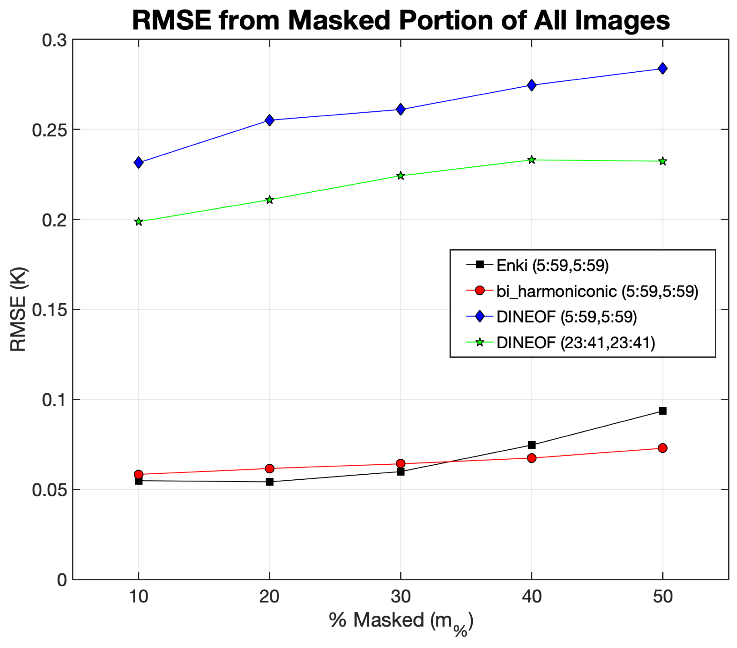
We begin our benchmark tests of Enki by comparing the Enki results to those from DINEOF (Data Interpolating Empirical Orthogonal Functions) [14], termed the gold-standard by Ćatipović et al. [12] based on the large fraction of manuscripts they reviewed in which it is used. Because DINEOF is based on an Empirical Orthogonal Function (EOF) analysis of the fields, we elected to use as our test dataset, a 180-day sequence of LLC4320 cutouts centered on (lat, lon) = ( 21 ° N, 118 ° E) in the South China Sea. Each cutout in the time series was masked using random 4 × 4 pixel patches obscuring a given fraction of the image m % . This was repeated for m % = [10%, 20% ...50%] and the t % = 20 model was used for the Enki reconstructions. The results are shown in Figure 7. Because the Enki reconstruction is based on surrounding pixels, a four-pixel-wide band at the edge of the cutout was excluded from the calculation of the RMSE for both reconstructions. A monotonic decrease in RMSE was found for the DINEOF reconstructions with increasing width of the excluded band. As an example of this, the RMSE of the DINEOF reconstruction excluding a 23-pixel band on the outer edge of the cutout is shown in Figure 7. The same is not true for the Enki and the biharmonic reconstructions (the latter discussed in the next section). Reconstruction errors are not shown for varying bands of Enki or the biharmonic method in the figure; with the exception of bands smaller than four pixels, the curves are indistinguishable from those of the four-pixel wide band.
Similar to published results with DINEOF, we recover an average RMSE of 0.25 K, weakly dependent on m % . In contrast, the Enki reconstructions have an RMSE 0.05 ; i.e., 5 × lower on average than the DINEOF algorithm. We also emphasize that first results using a convolutional neural network (DINCAE [17]) yield RMSE values similar to DINEOF. Therefore, the ViTMAE approach of Enki offers a qualitative advance over traditional deep-learning vision models.
As an alternative comparison, we have also calculated the Structural Similarity Index Measure (SSIM) on the reconstructed images, limiting the calculation to the reconstructed pixels. We find that the Enki yields values very close to 1 whereas DINEOF has SSIM 0.75 . We conclude that Enki significantly outperforms DINEOF in this metric.

3.6. Enki Performance Compared with Other Inpainting Algorithms—LLC4320 Cutouts

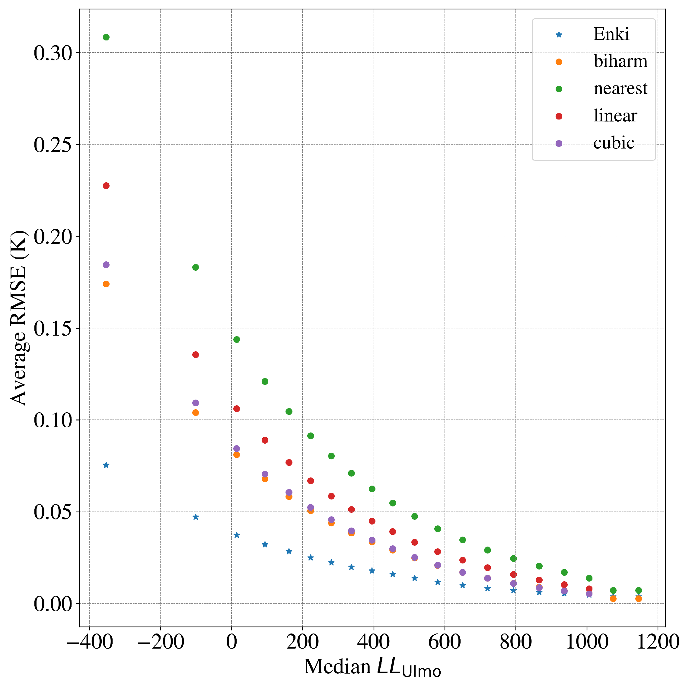
In addition to DINEOF, Ćatipović et al. [12] review a wide variety of other approaches, adopted by the community, to reconstruct remote sensing data. While a complete comparison to these is beyond the scope of this manuscript, we present additional tests here. Figure 8 shows the results, applied to the full validation dataset consisting of 655 , 000 cutouts, of several of these interpolation schemes—more easily implemented than either DINEOF or Enki—as a function of cutout complexity gauged by the L L Ulmo metric. Of these, the most effective is the biharmonic inpainting algorithm adopted in our previous work [9]. The figure shows, however, that Enki outperforms even this method by a factor of 2 to 3× in average RMSE aside from the featureless cutouts ( L L Ulmo > 300 ).
We also applied biharmonic inpainting to the 180-day sequence in the South China Sea discussed in the previous section, red circles in Figure 7. For this subset of the data, Enki performs slightly better than biharmonic inpainting for m % 30 while biharmonic inpainting appears to perform slightly better for larger values of m % (As with Enki the average RMSE was determined excluding a four-pixel-wide band around the edge of the cutout).
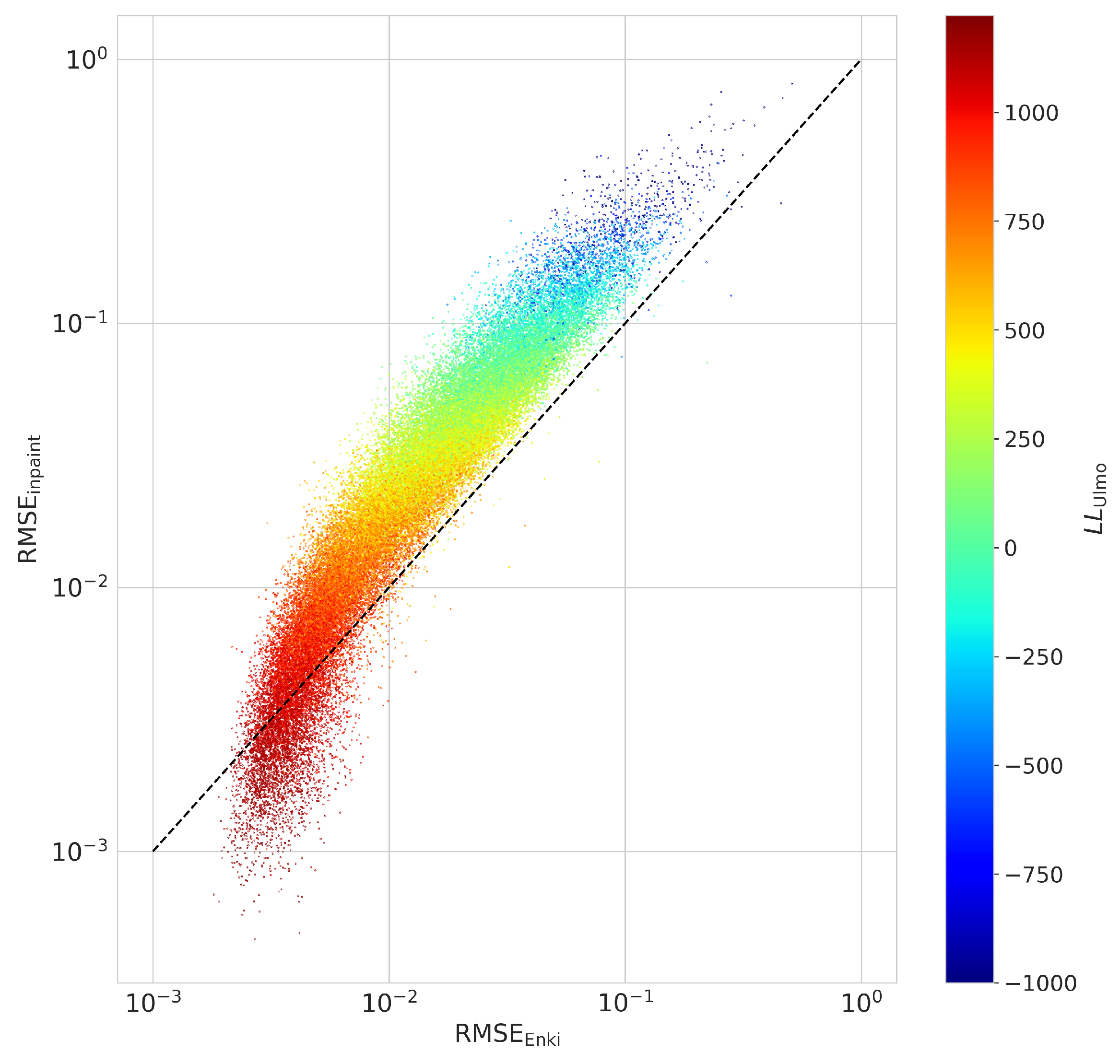
We explore the dependence on L L Ulmo in more detail in Figure 9, a scatter plot of RMSE for biharmonic inpainting versus RMSE for Enki, for all 650+ thousand LLC4320 cutouts examined. Colors in the figure denote L L Ulmo , a measure of image complexity, with lower values corresponding to more complexity. In >99.9% of the cases, Enki outperforms biharmonic inpainting, and often by more than an order-of-magnitude. This relationship holds independent of the image complexity for L L Ulmo < 750 . At L L Ulmo > 750 , which corresponds to cutouts with very little structure, the biharmonic algorithm yields lower RMSE than Enki. We hypothesize that there are small correlations in the model output that Enki has not learned and are better fit by the interpolation scheme. In real data, however, the differences between the two approaches would be overwhelmed by sensor noise.

3.7. Enki Performance—VIIRS SST Fields

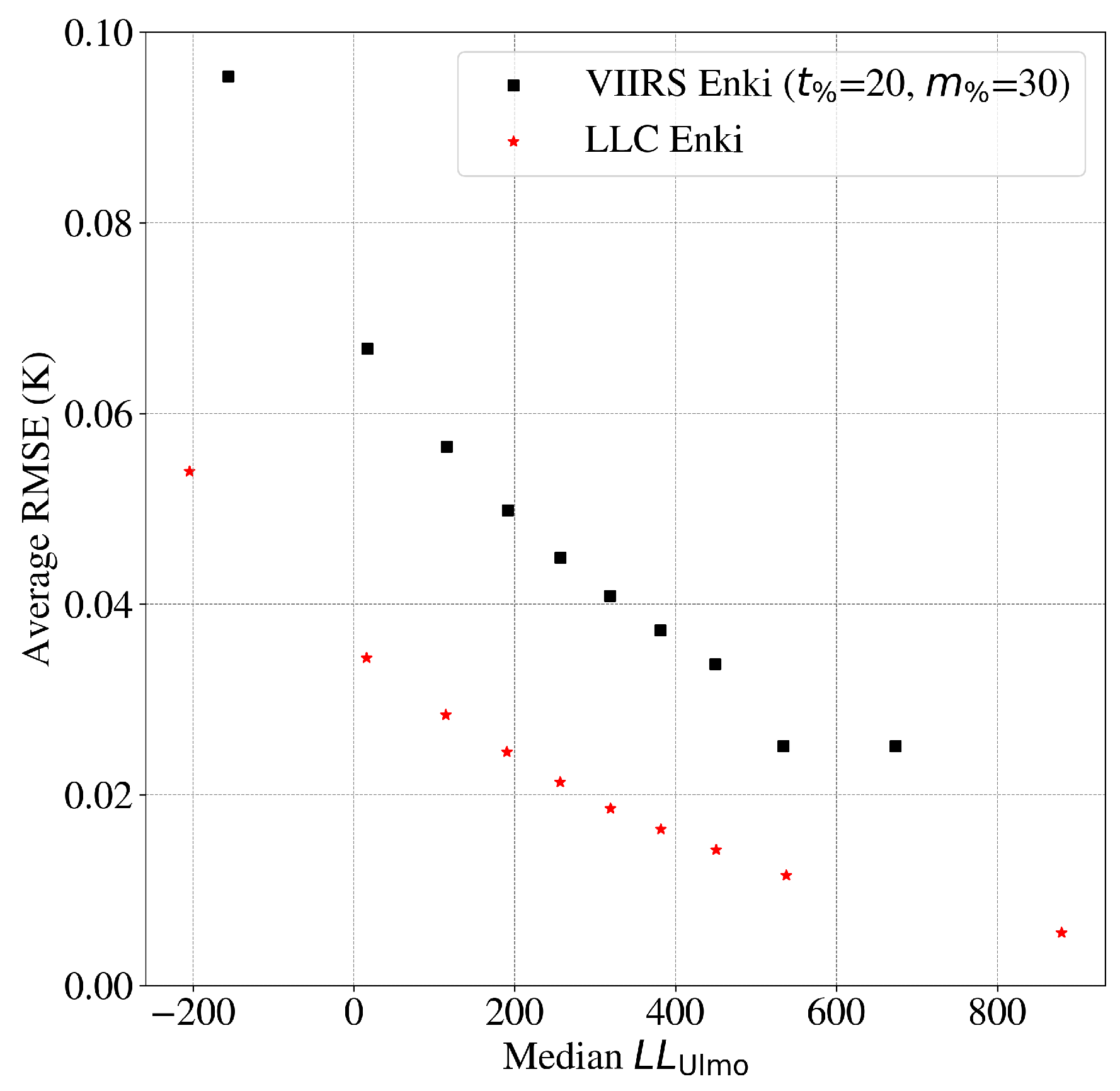
As a proof of concept for reconstructing real data, we applied Enki to the VIIRS dataset described in Section 2. For this exercise, we inserted randomly distributed clouds into cloud-free data, each with a size of 4 × 4 pixels. Figure 10 shows that the average RMSE values for Enki are less than sensor error ( RMSE VIIRS < ϵ VIIRS ) for cutouts with all complexity. The VIIRS reconstructions, however, do show higher average RMSE than those on the LLC4320 validation dataset. A portion of the difference is because the latter does not include sensor noise, which Enki has (sensibly) not been trained to recreate. We attribute additional error to the fact that the unmasked data also suffers from sensor noise (see Appendix A). And, we also anticipate a portion of the difference is because the VIIRS data have a higher spatial resolution than the LLC4320 model. Future experiments with higher-resolution models will test this hypothesis.

4. Conclusions

Satellite measurements are crucial for understanding the Earth’s climate system, requiring global and daily observations of the atmosphere, ocean, and land to comprehend their interactions. Currently, only space-based sensors can provide such comprehensive coverage, with our short-term predictive capabilities of these interactions relying heavily on current and historical satellite data. The Global Climate Observing System (GCOS), supported by international organizations, aims to ensure essential climate data, including 54 Essential Climate Variables (ECVs), are available, with satellites capable of measuring 26 of these ECVs. However, atmospheric conditions often limit satellite visibility to about 15% of the Earth’s surface at any time, posing significant challenges to climate science and prediction.
This study introduced Enki, a novel method to address data gaps in SST measurements using a NLP algorithm trained on ocean model outputs for image reconstruction. We have demonstrated that the Enki algorithm has reconstruction errors less than approximately 0.1 K for images with up to 50% missing data. That is, the RMSE is comparable or less than typical sensor noise. Furthermore, Enki outperforms other widely adopted approaches by up to an order of magnitude in RMSE, especially for fields with significant SST structure. Systems built upon Enki (or perhaps future algorithms like it) may therefore represent an optimal approach to mitigating masked pixels in remote sensing data.
An immediate application of Enki is the improvement of more than 40 years of SST measurements made by polar-orbiting and geosynchronous spacecraft [36]. In addition to reduction in geographic and seasonal biases [9,31], improvement of these datasets would likely translate to enhanced time series analysis and teleconnections between Essential Climate Variables (ECVs) across the globe. One objective of the present work, for example, is the improvement of L2 (i.e., swath) SST from the MODerate-resolution Imaging Spectroradiometer (MODIS), a high-resolution (1 km pixels, twice daily) data record that extends from 2000 to the present. Additionally, we anticipate integrating portions of the Enki encoder within comprehensive deep-learning models (e.g., [38]) in order to predict dynamical processes and extrema at the ocean’s surface.
The optimal performance of Enki may be achieved by iterative application of models with a range of t % and/or trained on specific geographical locations. At the minimum, improvements in the present approach will require models that accommodate a wider range of spatial scales and resolution than has been considered here (e.g., [39]). This is necessary, for example, to accommodate geostationary SST estimates, which have spatial resolutions closer to 5–10 km. We anticipate such improvements are straightforward to implement and are the focus of future work. Finally, we emphasize that the work presented here may be generalized to any remote sensing datasets in which a global corpus of realistic numerical output is available. In the oceanic context, this dataset might be ocean wind vectors, sea surface salinity, ocean color and—with improved biogeochemical modeling—even phytoplankton.
As noted in the introduction, Goh et al. [19] introduce a similar algorithm, which they refer to as MAE for SST Reconstruction under Occlusion (MAESSTRO). Although the algorithms are similar, the approach to validation of the results is quite different, effectively complimenting one another. We encourage those interested in implementing this approach to consider both pieces of work.

Author Contributions

Conceptualization, A.A. and J.X.P.; methodology, J.X.P. and A.A.; software, A.A. and J.X.P.; validation, all; formal analysis, all; investigation, A.A.; resources, J.X.P.; writing—original draft preparation, all; visualization, all; supervision, J.X.P.; project administration, J.X.P.; funding acquisition, A.A. All authors have read and agreed to the published version of the manuscript.

Funding

This research was funded by NASA grants 80NSSC18K0837 and 80NSSC20K1728 to P.C.C. and a Simons Foundation Pivot Fellowship to J.X.P.

Data Availability Statement

At the time of publication, all data products analyzed and produced by this project will be available in the Dryad archival system. All of the software is available at: https://github.com/AI-for-Ocean-Science/enki (accessed on 11 June 2024).

Acknowledgments

J.X.P. acknowledges support from the Simons Foundation. We thank David Reiman (Deep Mind) for inspiring this work, and Edwin Goh for his contributions in discussions on hyperparameters and early results. The authors acknowledge use of the Nautilus cloud computing system which is supported by the following US National Science Foundation (NSF) awards: CNS-1456638, CNS-1730158, CNS-2100237, CNS-2120019, ACI-1540112, ACI-1541349, OAC-1826967, OAC-2112167. VIIRS Data: The NOAA Office of Satellite and Product Operations (OSPO). 2014. GHRSST Level 2P NOAA/ACSPO SST from VIIRS on the S-NPP. Ver. 2.3. PO.DAAC, CA, USA. Dataset accessed [1 March 2023] at https://doi.org/10.5067/GHVRS-2PO02. LLC4320 Data: The LLC4320 SST fields were obtained via the xmitgcm package obtained at: https://xmitgcm.readthedocs.io/en/latest/.

Conflicts of Interest

The authors declare no conflicts of interest.

Abbreviations and Acronyms

The following abbreviations and acronyms are used in this manuscript:
AVHRRAdvanced Very-High-Resolution Radiometer
DINEOFData Interpolating Empirical Orthogonal Functions
ECCOEstimating the Circulation and Climate of the Ocean
ECMWFEuropean Centre for Medium-range Weather Forecasting
ECVEssential Climate Variable
EMelectromagnetic
EOFEmpirical Orthogonal Function
GCOSGlobal Climate Observing System
GPUGraphics Processing Unit
IRinfrared
L2Level-2
L4Level-4
LLCLatitude/Longitude/polar-Cap
LLC4320Latitude/Longitude-Cap-4320
MAESSTROMAE for SST Reconstruction under Occlusion
MITgcmMIT General Circulation Model
MLmachine learning
MODISMODerate-resolution Imaging Spectroradiometer
NLPnatural language processing
NOAANational Oceanic and Atmospheric Administration
RMSEroot mean square error
SSIMStructural Similarity Index Measure
SSTsea surface temperature
SSTaSST anomalies
SWOTSurface Water and Ocean Topography
TIROSTelevision InfraRed Observation Satellite
VIIRSVisible-Infrared Imager-Radiometer Suite
ViTMAEvision transformer masked autoencoder

Appendix A. Impacts of Sensor and Retrieval Noise on the Performance of Enki

To better understand the RMSE vs. σ T trends of Figure 4b and the impacts of noise on Enki reconstructions of masked areas in SST fields, we decompose both RMSE and σ T into contributing components.
For satellite-derived SST fields, patch complexity (herein denoted by σ T ) is a function of both (1) noise in the patch resulting from the instrument or noise introduced as part of the retrieval process σ n o i s e _ o _ i n and (2) geophysical structure within the field σ g e o _ o _ i n ; i.e., the signal of interest in the reconstruction. In these subscripts, the nomenclature “ _ o _ i n ” signifies that these terms relate to the original field and that the σ values correspond to the SST field inside the patch. The reasons for this distinction will become clear below.
Using these definitions, we can express the signal variance of the patch as
σ T 2 = σ n o i s e _ o _ i n 2 + σ g e o _ o _ i n 2 + 2 σ n o i s e _ o _ i n , g e o _ o _ i n 2
where σ g e o _ o _ i n is a function of the structure of the field, which we designate as ξ o _ i n , and σ n o i s e _ o _ i n , g e o _ o _ i n 2 is the covariance between the sensor/retrieval noise and geophysical signal. If we assume negligible correlation between the two sources of variability, then we approximate
σ T 2 σ n o i s e _ o _ i n 2 + σ g e o _ o _ i n 2 ,
Moreover, the root mean squared error (RMSE) of the prediction, which constitutes our measure of the quality of the reconstructed image, is given by
RMSE 2 ( σ n o i s e _ o _ i n , ξ o _ i n , σ n o i s e _ p _ i n , ξ p _ i n ) = σ n o i s e _ o _ i n 2 + σ n o i s e _ p _ i n 2 + f ( ξ o _ i n , ξ p _ i n )
where the subscript _ p references the predicted field, _ o u t refers to the characteristic, either noise or the geophysical signal, outside of the masked areas, and f ( ξ o _ i n , ξ p _ i n ) is the contribution to RMSE 2 resulting from the difference between the geophysical structure of the original field and that of the predicted field in the masked areas. Because Enki was trained on effectively noise-free model outputs (numerical noise will be negligible), we ignore σ n o i s e _ p _ i n hereafter. We also emphasize that the predicted geophysical variability ξ p _ i n is a function of the noise and geophysical structure in the original field (i.e., outside the masked pixels):
ξ p _ i n = ξ p _ i n ( σ n o i s e _ o _ o u t , ξ o _ o u t ) .
While this complex dependence can make interpretation of RMSE vs. σ T curves challenging, we offer the following discussion to aid the reader.
Figure A1. Investigation of the reconstruction error in individual 4 × 4 pixel patches as a function of σ T the measured standard deviation within the patch. For all of the datasets examined, we adopt the t % = 10 Enki model with m % = 10 masking. The blue circles are for the noiseless ( σ n o i s e _ o _ i n = σ n o i s e _ o _ o u t = 0 K) LLC4320 validation dataset similar to Figure 4b. The green stars is the same dataset with but with imputed white noise ( σ n o i s e _ o _ i n = σ n o i s e _ o _ o u t = 0.4 K). This curve follows the one-to-one line for σ T < σ n o i s e _ o _ i n as expected and then recovers toward the noiseless case as where the geophysical signal dominates σ T . The yellow triangles, meanwhile, show results where noise was imputed in the unmasked patches but ignored when measuring RMSE ( σ n o i s e _ o _ i n = 0 K, σ n o i s e _ o _ o u t = 0.4 K). The difference between this case and the noiseless dataset describes the impact of noise in the unmasked data for reconstruction. Last, the magenta squares show results for the VIIRS dataset. See the text for additional discussion on those results.
Remotesensing 16 02439 g0a1
The blue markers in Figure A1 correspond to the noise-free case (i.e., σ n o i s e _ o _ i n = σ n o i s e _ o _ o u t = 0 ):
RMSE 2 = f ( ξ o _ i n , ξ p _ i n ( 0 , ξ o _ o u t ) ) .
In the present context, this corresponds to the case where the original field is model SST. We attribute the flat portion of the curve up to σ T 10 2 K to two effects. The first is the limited precision of the ViTMAE tokenization of the patches; here we have adopted a 256-dimension latent vector. The other effect is a correlation between the size of geophysical structures and the magnitude of σ T . Specifically, for σ T 0.02 K the spatial scale of oceanographic features is in the order of or smaller than the 4 × 4 pixel patch size (i.e., 8 × 8 km2), such that there is little to no information available to reconstruct the structure in the masked area. As σ T increases above these values, the spatial scale of the features increases, with more information in the surrounding field available to reconstruct the field within the patch.
But the above analysis and interpretation are free from noise typically encountered in satellite-derived measurements. As previously mentioned, this can occur either due sensor noise or errors due to limitations of the retrieval algorithms used to estimate SST from the measured radiance. To investigate the impact of sensor and retrieval noise on Enki’s reconstructions, we add 0.04 K white Gaussian noise to the LLC4320 cutouts ( σ n o i s e _ o _ i n = σ n o i s e _ o _ o u t = 0.04 K in the above nomenclature) giving
RMSE 2 = ( 0.04 K ) 2 + f ( ξ o _ i n , ξ p _ i n ( 0.04 K , ξ o _ o u t ) ) .
We then repeat the analysis. Not surprisingly, the new results (green stars in Figure A1) follow the 1:1 line up to σ T of approximately 0.04 K, after which the RMS difference between the masked portions of the reconstructed SST fields and the underlying SST fields, to which 0.04 K Gaussian noise was also added, becomes progressively smaller than σ T . For σ T 0.04 K, the added noise tends to obscure the geophysical structure of the field. As σ T increases, however, the structure in the field eventually overwhelms the added noise and the improvement in reconstruction approaches that achieved with no noise added—i.e., the blue circles in Figure A1.
Also shown in Figure A1 is a similar set of points for VIIRS cutouts, the magenta squares. This curve follows neither the LLC4320 curve without noise (blue circles) nor the LLC4320 curve with noise (green stars). We believe that this results from the non-Gaussian nature of the noise in the VIIRS cutouts. To explore this, we repeat the above analysis except for σ n o i s e _ o _ i n = 0 and σ n o i s e _ o _ o u t = 0.04 K ; i.e.,
RMSE 2 = σ n o i s e _ p _ i n 2 ( 0.04 K , ξ o _ o u t ) + f ( ξ o _ i n , ξ p _ i n ( 0.04 K , ξ o _ o u t ) ) ,
which results in the yellow triangles in Figure A1. The added noise in this case only contributes to RMSE via Enki’s reconstructed fields; the difference between the blue circles (Equation (A5)) and yellow triangles (Equation (A7)) is a measure of the impact of the noise added to the region outside of masked areas on Enki’s reconstructed fields in masked areas. This curve is more similar to the VIIRS curve than the curves for either of the other two cases, no-noise (Equation (A5)) or Gaussian noise (Equation (A6)), for 10 3 σ T 2 × 10 1 K, the range including in excess of 80% of cutouts. This suggests that the noise in the VIIRS fields is not Gaussian. The two primary contributors to non-Gaussian VIIRS noise are (1) instrument noise (VIIRS is a multi-detector instrument and this can introduce noise in the along-track direction at harmonics corresponding to the number of detectors) and (2) clouds that were not properly masked by the retrieval algorithm. Clouds that have not been properly masked tend to result in cold anomalies, often substantially colder than the surrounding cloud-free region, which are structurally incompatible with geophysical processes. Furthermore, such anomalies tend to be relatively small in area—5 to 20 pixels—and in number (We were surprised by the significant fraction of cutouts in the VIIRS, “cloud-free” product we are using that are affected in this fashion). Although both of these sources of non-Gaussian noise may contribute to the shape of the VIIRS RMSE vs. σ T curve we believe that the primary problem is related to improperly masked clouds or other small scale atmospheric phenomena, which imprint themselves on the SST field as part of the retrieval.
In the above, we have shown how noise in the area surrounding masked pixels affects Enki’s ability to reconstruct the masked portion of the field. While not a major focus of this work, we have also suggested that non-Gaussian noise in VIIRS SST fields due to clouds, which have not been properly masked, is likely the primary cause of the degradation in Enki’s ability to reconstruct masked portions of these data.

References

  1. NASA. Space-Based Remote Sensing of the Earth: A Report to the Congress; NASA: Washington, DC, USA, 1987.
  2. Hovis, W.A.; Clark, D.K.; Anderson, F.; Austin, R.W.; Wilson, W.H.; Baker, E.T.; Ball, D.; Gordon, H.R.; Mueller, J.L.; El-Sayed, S.Z.; et al. Nimbus-7 Coastal Zone Color Scanner: System Description and Initial Imagery. Science 1980, 210, 60–63. [Google Scholar] [CrossRef] [PubMed]
  3. Huang, N.E.; Leitao, C.D.; Parra, C.G. Large-scale Gulf Stream frontal study using Geos 3 radar altimeter data. J. Geophys. Res. Ocean. 1978, 83, 4673–4682. [Google Scholar] [CrossRef]
  4. Born, G.H.; Dunne, J.A.; Lame, D.B. Seasat Mission Overview. Science 1979, 204, 1405–1406. [Google Scholar] [CrossRef] [PubMed]
  5. Fu, L.L.; Lee, T.; Liu, W.T.; Kwok, R. 50 Years of Satellite Remote Sensing of the Ocean. Meteorol. Monogr. 2019, 59, 5.1–5.46. [Google Scholar] [CrossRef]
  6. Stewart, R.H. Methods of Satellite Oceanography; Number 1 in Scripps Studies in Earth and Ocean Sciences; University of California Press: Berkeley, CA, USA, 1985. [Google Scholar]
  7. Robinson, I.S. Measuring the Oceans from Space: The Principles and Methods of Satellite Oceanography; Springer-Praxis Books in Geophysical Sciences; OCLC: ocm53926711; Springer-Praxis Pub: Berlin/Heidelberg, Germany; New York, NY, USA; Chichester, UK, 2004. [Google Scholar]
  8. Martin, S. An Introduction to Ocean Remote Sensing, 2nd ed.; Cambridge University Press: New York, NY, USA, 2014. [Google Scholar]
  9. Prochaska, J.X.; Cornillon, P.C.; Reiman, D.M. Deep Learning of Sea Surface Temperature Patterns to Identify Ocean Extremes. Remote Sens. 2021, 13, 744. [Google Scholar] [CrossRef]
  10. Reynolds, R.W.; Smith, T.M.; Liu, C.; Chelton, D.; Casey, K.S.; Schlax, M.G. Daily High-Resolution-Blended Analyses for Sea Surface Temperature. J. Clim. 2007, 20, 5473–5496. [Google Scholar] [CrossRef]
  11. NASA/JPL. GHRSST Level 4 MUR Global Foundation Sea Surface Temperature Analysis (v4.1); NASA/JPL: Pasadena, CA, USA, 2015. [CrossRef]
  12. Ćatipović, L.; Matić, F.; Kalinić’, H. Reconstruction Methods in Oceanographic Satellite Data Observation–A Survey. J. Mar. Sci. Eng. 2023, 11, 340. [Google Scholar] [CrossRef]
  13. Beckers, J.M.; Rixen, M. EOF Calculations and Data Filling from Incomplete Oceanographic D atasets. J. Atmos. Ocean. Technol. 2003, 20, 1839–1856. [Google Scholar] [CrossRef]
  14. Alvera-Azcárate, A.; Barth, A.; Rixen, M.; Beckers, J. Reconstruction of incomplete oceanographic data sets using empirical orthogonal functions: Application to the Adriatic Sea surface temperature. Ocean Model. 2005, 9, 325–346. [Google Scholar] [CrossRef]
  15. Alvera-Azcárate, A.; Barth, A.; Beckers, J.M.; Weisberg, R.H. Multivariate reconstruction of missing data in sea surface temperature, chlorophyll, and wind satellite fields. J. Geophys. Res. Ocean. 2007, 112. [Google Scholar] [CrossRef]
  16. Ping, B.; Su, F.; Meng, Y. An Improved DINEOF Algorithm for Filling Missing Values in Spatio-Temporal Sea Surface Temperature Data. PLoS ONE 2016, 11, e0155928. [Google Scholar] [CrossRef] [PubMed]
  17. Barth, A.; Alvera-Azcárate, A.; Licer, M.; Beckers, J.M. DINCAE 1.0: A convolutional neural network with error estimates to reconstruct sea surface temperature satellite observations. Geosci. Model Dev. 2020, 13, 1609–1622. [Google Scholar] [CrossRef]
  18. Larson, A.; Akanda, A.S. Transforming Observations of Ocean Temperature with a Deep Convolutional Residual Regressive Neural Network. arXiv 2023, arXiv:2306.09987. [Google Scholar]
  19. Goh, E.; Yepremyan, A.R.; Wang, J.; Wilson, B. MAESSTRO: Masked Autoencoders for Sea Surface Temperature Reconstructi on under Occlusion. EGUsphere 2023, 2023, 1–20. [Google Scholar] [CrossRef]
  20. He, K.; Chen, X.; Xie, S.; Li, Y.; Dollár, P.; Girshick, R.B. Masked Autoencoders Are Scalable Vision Learners. In Proceedings of the IEEE/CVF Conference on Computer Vision and Pattern Recognition (CVPR), New Orleans, LA, USA, 18–24 June 2022. [Google Scholar]
  21. Marshall, J.; Adcroft, A.; Hill, C.; Perelman, L.; Heisey, C. A finite-volume, incompressible Navier-Stokes model for studies of the ocean on parallel computers. J. Geophys. Res. 1997, 102, 5753–5766. [Google Scholar] [CrossRef]
  22. Marshall, J.; Hill, C.; Perelman, L.; Adcroft, A. Hydrostatic, quasi-hydrostatic, and nonhydrostatic ocean modeling. J. Geophys. Res. 1997, 102, 5733–5752. [Google Scholar] [CrossRef]
  23. Adcroft, A.; Campin, J.M.; Hill, C.; Marshall, J. Implementation of an Atmosphere–Ocean General Circulation Model on the Expanded Spherical Cube. Mon. Weather Rev. 2004, 132, 2845–2863. [Google Scholar] [CrossRef]
  24. Rocha, C.B.; Chereskin, T.K.; Gille, S.T.; Menemenlis, D. Mesoscale to submesoscale wavenumber spectra in Drake Passage. J. Phys. Oceanogr. 2016, 46, 601–620. [Google Scholar] [CrossRef]
  25. Su, Z.; Wang, J.; Klein, P.; Thompson, A.F.; Menemenlis, D. Ocean submesoscales as a key component of the global heat budget. Nat. Commun. 2018, 9, 775. [Google Scholar] [CrossRef]
  26. Torres, H.S.; Klein, P.; Menemenlis, D.; Qiu, B.; Su, Z.; Wang, J.; Chen, S.; Fu, L.L. Partitioning Ocean Motions Into Balanced Motions and Internal Gravity Waves: A Modeling Study in Anticipation of Future Space Missions. J. Geophys. Res. Ocean. 2018, 123, 8084–8105. [Google Scholar] [CrossRef]
  27. Savage, A.C.; Arbic, B.K.; Alford, M.H.; Ansong, J.K.; Farrar, J.T.; Menemenlis, D.; O’Rourke, A.K.; Richman, J.G.; Shriver, J.F.; Voet, G.; et al. Spectral decomposition of internal gravity wave sea surface height in global models. J. Geophys. Res. Ocean. 2017, 122, 7803–7821. [Google Scholar] [CrossRef]
  28. Arbic, B.K.; Alford, M.H.; Ansong, J.K.; Buijsman, M.C.; Ciotti, R.B.; Farrar, J.T. A Primer on Global Internal Tide and Internal Gravity Wave Continuum Modeling in HYCOM and MITgcm; New Frontiers In Operational Oceanography, GODAE OceanView; FSU: Tallahassee, FL, USA, 2018; Chapter 13; pp. 307–392. [Google Scholar] [CrossRef]
  29. Wang, J.; Fu, L.L.; Qiu, B.; Menemenlis, D.; Farrar, J.T.; Chao, Y.; Thompson, A.F.; Flexas, M.M. An Observing System Simulation Experiment for the Calibration and Validation of the Surface Water Ocean Topography Sea Surface Height Measurement Using In Situ Platforms. J. Atmos. Ocean. Technol. 2018, 35, 281–297. [Google Scholar] [CrossRef]
  30. Forget, G.; Campin, J.M.; Heimbach, P.; Hill, C.N.; Ponte, R.M.; Wunsch, C. ECCO version 4: An integrated framework for non-linear inverse modeling and global ocean state estimation. Geosci. Model Dev. 2015, 8, 3071–3104. [Google Scholar] [CrossRef]
  31. Gallmeier, K.; Prochaska, J.X.; Cornillon, P.C.; Menemenlis, D.; Kelm, M. An evaluation of the LLC4320 global ocean simulation based on the submesoscale structure of modeled sea surface temperature fields. arXiv 2023, arXiv:2303.13949. [Google Scholar] [CrossRef]
  32. Yu, X.; Ponte, A.L.; Elipot, S.; Menemenlis, D.; Zaron, E.D.; Abernathey, R. Surface Kinetic Energy Distributions in the Global Oceans from a High-Resolution Numerical Model and Surface Drifter Observations. Geophys. Res. Lett. 2019, 46, 9757–9766. [Google Scholar] [CrossRef]
  33. Arbic, B.K.; Elipot, S.; Brasch, J.M.; Menemenlis, D.; Ponte, A.L.; Shriver, J.F.; Yu, X.; Zaron, E.D.; Alford, M.H.; Buijsman, M.C.; et al. Near-Surface Oceanic Kinetic Energy Distributions from Drifter Observations and Numerical Models. J. Geophys. Res. Ocean. 2022, 127, e2022JC018551. [Google Scholar] [CrossRef]
  34. Jonasson, O.; Ignatov, A. Status of second VIIRS reanalysis (RAN2). In Proceedings of the Ocean Sensing and Monitoring XI, Baltimore, MD, USA, 16–18 April 2019; Hou, W.W., Arnone, R.A., Eds.; International Society for Optics and Photonics. SPIE: Bellingham, WA, USA, 2019; Volume 11014, p. 110140O. [Google Scholar] [CrossRef]
  35. Prochaska, J.X.; Guo, E.; Cornillon, P.C.; Buckingham, C.E. The Fundamental Patterns of Sea Surface Temperature. arXiv 2023, arXiv:2303.12521. [Google Scholar] [CrossRef]
  36. Agabin, A.; Prochaska, J.X. Reconstructing Sea Surface Temperature Images: A Masked Autoencoder Approach for Cloud Masking and Reconstruction. arXiv 2023, arXiv:2306.00835. [Google Scholar] [CrossRef]
  37. Wu, F.; Cornillon, P.; Boussidi, B.; Guan, L. Determining the Pixel-to-Pixel Uncertainty in Satellite-Derived SST Fields. Remote Sens. 2017, 9, 877. [Google Scholar] [CrossRef]
  38. Tseng, G.; Zvonkov, I.; Purohit, M.; Rolnick, D.; Kerner, H. Lightweight, Pre-trained Transformers for Remote Sensing Timeseries. arXiv 2023, arXiv:2304.14065. [Google Scholar]
  39. Reed, C.J.; Gupta, R.; Li, S.; Brockman, S.; Funk, C.; Clipp, B.; Keutzer, K.; Candido, S.; Uyttendaele, M.; Darrell, T. Scale-MAE: A Scale-Aware Masked Autoencoder for Multiscale Geospatial Representation Learning. arXiv 2023, arXiv:2212.14532. [Google Scholar]
Figure 1. Architecture of our ViTMAE named Enki. To train the algorithm, a cloud-free image is broken down into patches, a fraction of which are randomly selected in the image and masked. For simplicity, this example shows a 64 × 64 pixel image with 16 × 16 pixel patches, 40% of which are masked. (Enki actually operates on 64 × 64 pixel images with 4 × 4 pixel masks.) The unmasked patches are flattened and embedded by a linear projection with positional embeddings which are then run through the encoder, returning the encoded patches which are then run through the decoder along with the masked (unfilled) tokens. This returns another latent vector, and another linear projection layer outputs this vector as an image with the same dimensions of the original image. The asterisks represent the contents of each patch.
Remotesensing 16 02439 g001
Figure 2. An example of the Enki model applied to simulated data with masked or missing pixels. In this case, Enki was trained on realistic ocean model output consisting of 20% of pixels flagged as “poor” (masked) and applied to an image with 30% of pixels flagged as masked. The panels are: (a) original SSTa, (b) masked SSTa in 4 × 4 pixel patches covering 20% of the image, (c) reconstructed SSTa, and (d) residual (reconstruction minus truth). Ignoring the image boundary (see Section 3.2), the maximum reconstruction error is only 0.19 K and the highest RMSE in a single patch is 0.07 K with an average RMSE 0.02 K.
Remotesensing 16 02439 g002
Figure 3. Model bias. Median bias in the SST predicted by each model as a function of the training percentile t % and patch masking percentile m % . For large t % and small m % the model exhibits a significant bias with an unknown origin [36]. At lower t % , however, the bias reaches a nearly negligible value. Note that the value for t % = 10 are all at 0 K and below the t % = 20 points.
Remotesensing 16 02439 g003
Figure 4. Results for individual 4 × 4 pixel patches. Both panels present reconstruction results for the validation dataset using a masking percentile of m % = 30 and the t % = 20 Enki model. (a) Median RMSE as a function of the patch spatial location where i , j refers to the position of the lower-left corner of the patch. Patches on the image boundary exhibit systematically higher RMSE and we advocate ignoring these in any image reconstruction application. (b) Median of log 10 RMSE for patches as a function of log 10 of the standard deviation of SST ( σ T ) in the patch. For patches with non-negligible structure ( σ T > 10 2 K), the reconstruction RMSE is 10 × lower than random (as described by the dashed one-to-one line). The red curve is a two-parameter fit to the data.
Remotesensing 16 02439 g004
Figure 5. Enki’s reconstruction performance as a function of mask characteristics. (a) The difference in the RMSE between the true and reconstructed SST values as a function of the area of the masked region. Note that the horizontal axis is logarithmic. Masked regions exist in increments of 16 pixels—each mask consists of an integer number of joined 4 × 4 pixel regions. For each masked area bin, the 50th (median) and the mean calculated from the logarithm of the values is shown. Vertical gray bars—vertical scale to the right—define the histogram of the distribution of the cutouts by area bin. (b) Model performance as a function of the minor axis length of each cutout. This horizontal axis is also logarithmic.
Remotesensing 16 02439 g005
Figure 6. Enki’s reconstruction performance on the validation dataset. (a) Model performance as a function of quantiles of image complexity, L L Ulmo , with higher values indicating lower complexity. The reconstruction error is sensitive to the degree of structure in the field, although for masking percentile m % < 20 even the most complex images have RMSE 0.06 K. (b) Model performance as a function of masking percentile for the full set of trained Enki models. Contrary to expectation, we find the t % = 20 model outperforms all others at all m % . The poorer performance of the t % > 20 models at low m % indicates those models have not learned the small-scale features present in SST data.
Remotesensing 16 02439 g006
Figure 7. Average reconstruction error for a 180-day sequence of cutouts centered on lat, lon = 21 ° N, 118 ° E in the South China Sea for the DINEOF algorithm (blue diamonds), the biharmonic algorithm (red circles) and Enki (black squares) based on the cutout excluding a 4-pixel-wide band on the outer edge of the cutouts; i.e., from pixels 5 to 59 of the 64 pixels in the two directions. Green stars delineate the reconstruction error for DINEOF based on the cutouts excluding a band 21 pixels wide on the other edge of the each cutout; pixels 23 to 41 in the two directions.
Remotesensing 16 02439 g007
Figure 8. Comparison of the average RMSE for a series of interpolation schemes (circles) against the results from Enki. These are for reconstructions of the LLC4320 validation dataset using the t % = 20 model on data m % =30 masked patches. Aside from the nearly featureless cutouts ( L L Ulmo > 750 ), Enki well out-performs all of these schema and typically by factors of 3 to 5×.
Remotesensing 16 02439 g008
Figure 9. Comparison of reconstruction error for Enki (RMSEEnki) with the biharmonic inpainting algorithm (RMSEinpaint) on the validation dataset. Colors denote the L L Ulmo metric [9], which is a measure of image complexity; lower values indicate higher image complexity. The results here correspond to the t % = 20 model applied to data with m % = 30 masking.
Remotesensing 16 02439 g009
Figure 10. Enki performance on real sensor data. The black squares show the average RMSE for reconstructions of VIIRS images in bins of image complexity (higher L L Ulmo indicates less complexity). Even reconstructions of the most complex images ( L L Ulmo < 0 ) show the average RMSE is lower than the estimated sensor noise (≈0.1 K [37]). For comparison, we show the average RMSE values for Enki reconstructions of the LLC4320 validation data (red). All of the results adopt the Enki model trained with t % = 20 and applied to cutouts with m % = 30.
Remotesensing 16 02439 g010
Disclaimer/Publisher’s Note: The statements, opinions and data contained in all publications are solely those of the individual author(s) and contributor(s) and not of MDPI and/or the editor(s). MDPI and/or the editor(s) disclaim responsibility for any injury to people or property resulting from any ideas, methods, instructions or products referred to in the content.