Article

Anomaly Detection of Sensor Arrays of Underwater Methane Remote Sensing by Explainable Sparse Spatio-Temporal Transformer

1
National Key Laboratory of Advanced Micro and Nano Manufacture Technology, Shanghai Jiao Tong University, Shanghai 200240, China
2
Department of Micro/Nano Electronics, School of Electronic Information and Electrical Engineering, Institute of Marine Equipment, Shanghai Jiao Tong University, Shanghai 200240, China
*
Author to whom correspondence should be addressed.
Remote Sens. 2024, 16(13), 2415; https://doi.org/10.3390/rs16132415
Submission received: 18 April 2024 / Revised: 24 June 2024 / Accepted: 24 June 2024 / Published: 1 July 2024

Abstract

:
The increasing discovery of underwater methane leakage underscores the importance of monitoring methane emissions for environmental protection. Underwater remote sensing of methane leakage is critical and meaningful to protect the environment. The construction of sensor arrays is recognized as the most effective technique to increase the accuracy and sensitivity of underwater remote sensing of methane leakage. With the aim of improving the reliability of underwater methane remote-sensing sensor arrays, in this work, a deep learning method, specifically an explainable sparse spatio-temporal transformer, is proposed for detecting the failures of the underwater methane remote-sensing sensor arrays. The data input into the explainable sparse block could decrease the time complexity and the computational complexity (O (n)). Spatio-temporal features are extracted on various time scales by a spatio-temporal block automatically. In order to implement the data-driven early warning system, the data-driven warning return mechanism contains a warning threshold that is associated with physically disturbing information. Results show that the explainable sparse spatio-temporal transformer improves the performance of the underwater methane remote-sensing sensor array. A balanced F score (F1 score) of the model is put forward, and the anomaly accuracy is 0.92, which is superior to other reconstructed models such as convolutional_autoencoder (CAE) (0.81) and long-short term memory_autoencoder (LSTM-AE) (0.66).

1. Introduction

Combustible ice is a crystalline substance formed by methane and water under low temperature and high pressure, which is similar to ice in shape. The methane content of combustible ice can reach 99% at most, and one volume of combustible ice can store 100–200 times the volume of methane gas [1,2,3]. Combustible ice, often found in deep ocean sediments, is a highly efficient green energy source [4,5]. Its energy, generated by combustion, is ten times more than natural gas, gasoline, and coal, making it useful for a low-carbon society [6,7]. In addition, some underwater methane leakage occurrences create a negative influence on the environment, i.e., leakage from the Nordstream pipeline has caused pollution to the environment [8,9,10]. Therefore, underwater remote sensing of methane is of great importance for protecting the environment [11].
There are mainly two kinds of space methane telemetry: airborne and satellite detection [12]. The advantage of space methane telemetry is that it can detect methane in a large area over water, but the disadvantage is that it cannot detect methane in water. However, in terms of the effectiveness of their long-term utilization for methane exploration and pipeline leakage detection in the deep ocean, the output of a methane gas sensor could be easily affected by environmental factors, such as sway, shake, temperature, and pressure, as well as degradation of the sensor materials’ characteristics, such as heating of wires or oxidation. The above factors give rise to the deviation of detection data from the true value and the extraction of false data [13,14,15]. Aiming to improve the detection performance, sensor arrays with anomaly detection mechanisms have proven to be an effective solution in underwater methane remote sensing. For many years, researchers have been concerned with the data fusion anomaly detection of gas sensor arrays, and a number of intelligent sensors have been widely used in every field of the industry [16,17,18].
Anomaly detection is the observation value produced by the negligence error in the process of observations or tests that destroys the original statistical regularity. Anomaly data are generally significantly larger or smaller than other observations and are easily neglected. Anomaly detection is mainly solved by three methods: statistical model methods, anormal signal modeling methods, and reconstruction of normal signal methods. In anormal signal modeling approaches, a great deal of anomaly training data are required to model the signal. However, for anomaly data, their characteristics are generally complex and unknown, and their number is exceedingly small. This dilemma leads to certain limitations to the anomaly signal modeling methods, resulting in rare use for underwater methane remote sensing.
Statistical model methods, including the Gaussian regression method [19], Bayesian-based method [20,21], and density estimations based on local outlier factors [22], may rely on the data distribution in real conditions. Therefore, statistical models are also rarely applied in underwater methane remote sensing [23]. In contrast, the reconstruction of normal signal methods has relatively few restrictions [24,25,26,27,28]. Currently, the majority of normal signal reconstruction methods are mainly used to extract the continuous or discrete temporal features of the general signal [29,30,31,32,33]. A long-short term memory_autoencoder (LSTM_AE) model was proposed by Pankaj Malhotra et al. (2016) to detect multi-sensor abnormal data [34]. An unsupervised detection method was adopted by Xuan-hao Chen et al. (2021) for abnormal multivariate time series [35].
However, most normal signal reconstructions seldom take the spatial correlation of signals or images into consideration [36,37,38,39,40]. The temporal correlation information extracted by most reconstruction methods can only include partial information, and other abstract spatial information cannot be extracted. In complex industrial environments, such as deep ocean energy exploitation and motor vehicle engine health detection, the spatial analysis of these industrial signals may be unrecognized, and the signal reconstruction would decrease the anomaly detection accuracy [41,42]. Hence, it is urgent to produce an anomaly-monitoring model that can extract both temporal and spatial information in underwater methane remote sensing.
In this work, an explainable spatio-temporal transformer model was proposed for methane sensor array anomaly detection in underwater methane remote-sensing applications. The model used a data transfer method to distinguish normal data and anomaly data, which can significantly reduce the data required for the task. An attention block was proposed to automatically capture the spatial features of the gas sensor array signal and the temporal features, including temperature information, with a small amount of data. Furthermore, due to the redundancy of sensor array information, interpretable sparse attention is proposed, which can remove the time complexity during the modeling and improve the computational efficiency. In addition, a data-driven early warning device was added to our proposed model that could return the location of anomaly data. The key highlights of our work are as follows:
(1)
A classical self-attention mechanism was modified to lower the time complexity to O (n) by an explainable sparse block. The sparse block takes inspiration from graph sparsification methods and physical response features of sensor array data;
(2)
The traditional self-attention block was replaced by a spatio-temporal-enhanced attention block. This spatio-temporal attention block can automatically capture spatial characteristics of the gas sensor array signal with a query matrix and temporal features, including temperature information. This is accomplished with a key matrix, which is suitable for underwater methane remote sensing;
(3)
The anomaly detection threshold technology was set as a data-driven early warning system. This is an unsupervised method that removes the impact of the unknown anomaly signals of industrial sensor arrays to improve anomaly detection accuracy.
The basic framework of the paper is as follows. Section 2 includes the theoretical fundamentals, including the suggested deep learning neural network; Section 3 is a discussion of the experiment and the results; the following sections include the conclusion and future work.

2. Theoretical Fundamentals

2.1. Explainable Sparse Mask

Due to the computational complexity O (n2) of the original transformer [43,44], which can improve the cost of training the model, some interesting attempts have been performed to alleviate the quadratic dependency. The proposed explainable sparse mask was inspired by Luong et al. (2015) [45]. The proposed mask can lower the computational complexity to O (n) and is more suitable for industrial applications because of interpretable characteristics.
The first part is the window mask, displaying a large amount of locality of reference (Figure 1a). Self-attention models have been demonstrated by Clark et al. (2019) [46], and a measure of local connectivity of three was set as the clustering coefficient. According to Clark et al. (2019) [46], while creating the local attention block, index j of each query block serves as the key block, with the index being j − (w − 1)/2 to j + (w − 1)/2, where j is the key. Figure 1a shows that w = 3 with block size 2 implies every query block j attending to a key block j 1 ,   j , ( j + 1 ) .
The second piece of the mask is inspired by the global attention mechanism of Clark et al. (2019) [46], shown in Figure 1b, which is critical for empirical performance. More specifically, the importance of “global tokens” is adopted. Tokens that assist all tokens in the sequence and to whom all tokens attend are called global tokens, as shown in Figure 1c. The global tokens can be described as internal transformer construction (ITC). Several tokens available are set as “global”; these are involved in the whole sequence. Specifically, if a subset G of indices (with g: = |G|) is selected, for all i   G, A(i, :) = 1 and A(:, i) = 1 will be obtained. In this paper, the model computes it according to blocks g = 1 with block size 2.
The raised model is in view of the window mask and incorporates the characteristics of the sensor response, which makes the methods interpretable (Figure 1c). According to our original methane data, it can be found that the corresponding period is 50/300, our mask is 8 × 8, and the mapping to the mask becomes 1.33. We take 1 unit, and we remove the squares with the interval of 1 unit on the window mask, completing the construction of the sparse mask for interpretability.
The final attention mechanism for the explainable sparse mask in Figure 1d has both of these properties. W/2 tokens to the left and w/2 to the right of the location are attended by each query, and g global tokens are contained.
Algorithm 1 shows the explainable sparse mask process. The details are described above.
Algorithm 1 Explainable Sparse Mask
functionExplainable Sparse Mask (Xinput)
|QspatioXinput
| M a s k ( δ )     Sparse   Matrix   ( 8   8)
|Qmask     Q spatio     M a s k ( δ )
|return Qmask
End

2.2. Explainable Sparse Spatio-Temporal Attention

A review of the attention mechanism can be found in Supplementary S1. The attention-based framework of transformer can be found in Supplementary S2. Considering a lack of concentration in attention can result in the failure of relevant information extraction, an explainable sparse spatio-temporal transformer (ESST transformer) model is proposed. The ESST transformer is a mixed end-to-end structure focused on learning the spatio-temporal features based on time, which is an extension and expansion of the traditional transformer with only O (n) computational complexity. The proposed ESST transformer has three main procedures, which are the explainable sparse mask, time-distributed temporal feature selection, and comprehensive spatial feature extraction. A schematic diagram of the ESST transformer and a traditional self-attention module are shown in Figure 2.
Firstly, the holistic spatial features are extracted by the spatio attention block. The pooling layer can compress the original data, reduce the calculation parameters of the model, and improve the calculation efficiency. The spatio attention block learns the information between sensor arrays through spatial feature extraction. One of the commonly used layers is the average pooling layer; the other is the maximum pooling layer. The data processing of the pooling layer is normally the feature map of the generated layer after processing of the convolution layer.
For the spatio attention block by the pooling layer, the output size is
Q S p a t i o = A v g P o o l   ( Q o r i g i n a l )
A v g P o o l = ( x i n p u t _ s i z e + 2     p F ) / s ) + 1
QSpatio represents the size of the output, xinput_size represents the size of the input, F represents the size of the kernel, p represents padding (Default 0), and s represents stride (Default 1).
Then, the explainable sparse mask is used on QSpatio to reduce the computational complexity:
Q m a s k = M ( Q S p a t i o )
where M( ) represents the explainable sparse mask.
Temporal features are extracted after the softmax of the score between Qmask and Keys by the LSTM network.
T e m p o r a l   B l o c k   =   L S T M   [ S o f t m a x   ( S c o r e ( Q m a s k     k T ) ) ]
where Key is the classification information of the sensor array data.
The features mainly contain temperature drift information, which can influence the sensing accuracy of underwater methane remote sensing.
The spatial and temporal features of the sensing array information are first combined in this place. The combination of features can enhance the characteristics of spatio-temporal information to extract more abstract information and increase the accuracy of methane data reconstruction.
Enhanced spatio-temporal information is finally input into the matrix by V values that contain the whole information of sensor arrays. The significance of this part is in the integration of the enhanced spatio-temporal information with the initial global information. The spatio-temporal block lets the proposed attention acquire the global vision and local spatio-temporal vision. The formula of ESST attention is
E S S T   a t t e n t i o n   =   T e m p o r a l   B l o c k     v .
The total ESST attention mechanism is defined as
E S S T   a t t e n t i o n   =   L S T M h = 1 H δ A v g P o o l ( Q h ) · X n i K h T · V h
where Qh is the query function, Kh is the key function, Vh represents the value function, δ indicates a scoring function, such as softmax, and H is the number of heads, respectively. XN(i) corresponds to the matrix of the sparse mask.
Algorithm 2 shows the whole process of explainable sparse spatio-temporal attention. The details are described in Equations (1)–(5) above.
Algorithm 2 Explainable Sparse Spatio-Temporal Attention
functionESST Attention (Xinput)
|Q, K, VXLinearized
|QSpatio ← AvgPool (Q) (1,2)
|QmaskM(QSpatio)(3)
|Scorespatio = QmaskKT(4)
|Temporal Block = LSTM [Softmax (ScoreSpatio)]
| E = Temporal   Block    V(5)
|return  E
end

2.3. ESST Transformer Reconstruction Mechanism

2.3.1. ESST Transformer Model

Encoder: A pack of N = 3 identical layers is composed in the encoder. There are two sub-layers in each layer. The multi-head spatio-temporal attention mechanism is used in the first sublayer, and an effective and totally connected position-wise feed-forward network is applied in the second sublayer. A residual connection is utilized, and a layer normalization follows around each of the two sub-layers. This means that Layer-Norm (x + Sublayer(x)) is output, where the function validated by the sub-layer itself is noted as Sublayer(x). All sub-layers including the embedding layers in the model generate outputs with a dimension of dmodel = 16 to facilitate the residual connections
Decoder: A pack of identical layers of N = 3 is also composed in the decoder. Apart from both sub-layers of each encoder layer, the third one is inserted in the decoder, performing multi-head attention over the output of the encoder stack. Similarly, residual connections around each of the sub-layers are also employed, and normalization of the layers follows.
The spatio-temporal attention sub-layer is also modified in the decoder stack to protect positions against assisting subsequent positions. Regarding the fact that the output embeddings are counterbalanced by one position, this masking guarantees that position i can be predicted only by the given outputs of the locations less than i. The Encoder-Decoder block of anomaly detection is shown in Figure S1. The introduction of Figure S1 is shown in Supplementary S2.
Table 1 shows the parameters related to the anomaly detection. Considering the complexity of the anomaly data, it is necessary for sufficient attention to learn the coherence of data in the training process; hence, the head parameter is chopped to 2. The classical transformer model was used in the middle layer without any modifications. The dropout operation was employed in layer 3 and 4 to avoid the appearance of over fitting of the model during training, which could lead to poor performance during testing.

2.3.2. Data Reconstruction by Generative ESST Trans.

The original data are compared with the anomaly data by a data transfer method. The trained ESST model is adopted to reconstruct the signals with anomaly values. Figure 3 shows a signal reconstruction flowchart. Compared with unsupervised learning, such as reinforcement learning, this method requires less labeled data to train and works well, so as to reduce the data acquisition cost.
It is demonstrated in Figure 3 that in the signal reconstruction process, signals are input into the trained ESST transformer model and undergo each layer of the trained network to produce the reconfigured signals. The raw signal flow, involving normal defect signals, normal smooth signals, and anomaly signals, is fed into the first spatial encoder to select the first-level spatial features. The extracted features are input into the second temporal feature extractor along with the mean-pooled original signals. Correspondingly, the signal flow manages to run through the other feature extraction layers and the data recovery layers of the network. Sequentially processed by the ESST transformer, the reconstructed signals will be obtained.

2.4. Anomaly Signal Warning Systems

2.4.1. Traditional Anomaly Detection Methods

By contrasting the analyses of renewed signals and input signals, the defect signals and anomaly signals can be identified by a core step in anomaly signal detection. One of the factors affecting the detection accuracy rate is the design of an appropriate threshold.
The reconstructed error of each section can be obtained by Equation (7):
E i = A i C i 2
where Ai and Ci denote the ith input segment and the reconfigured segment, respectively, and Ei denotes the ith reconstruction error.

2.4.2. Adaptive Dynamic Threshold Design

In this section, an adaptive dynamic threshold scheme is designed to rely on the statistics of normal smooth signals and normal defect signals. This design has a strong robustness of anomaly detection through the addition of a lot of restrictions on the function, which avoids false alarms in the early warning process. At the same time, considering the effect of environmental factors on the detection accuracy, the detection threshold appropriately reduces the anomaly range so as to increase the anti-interference of the model to environmental factors.
The reconstruction error of normal smooth signals without defects is defined as En, and the values of anomaly signal reconstruction error are defined as Ea. In the threshold function, 0.8 is a hyperparameter that is obtained by data observation. The threshold T is determined by Equation (8):
T = 1 2 E n + E a ,   i f   E a > 0.8   and   2 E n < E a T = E a ,   i f   E n < E a
While the threshold T is obtained by (8), it is compared with the reconstruction error (ET), and the evaluation of normal defect signals and anomaly signals can be realized by Equation (9):
E T > T   : A n o m a l y   s i g n a l s E T T   : N o r m a l   s i g n a l s
Algorithm 3 shows the entire Anomaly Signal Warning system. The details are described in Formulas (8) and (9) above.
Algorithm 3 Anomaly Signal Warning Systems
functionAnomaly Detection (Xa, Xn)
|EaEn ← XaXn
|for iEa in range (Xa) do
||      for iEn in range (Xn) do
||          |            if   E a   >   0.8   and   2    (En) < Ea:(8)
||          |                          T     1 / 2    (En + Ea)
||          |          elif Ea > En:(8)
||          |                        T ← Ea
||      end
||         if Ea > T:(9)
||                  print (iEa)
|End
Return i, Ea

3. Experiment, Results, and Discussion

3.1. Experiment Setup

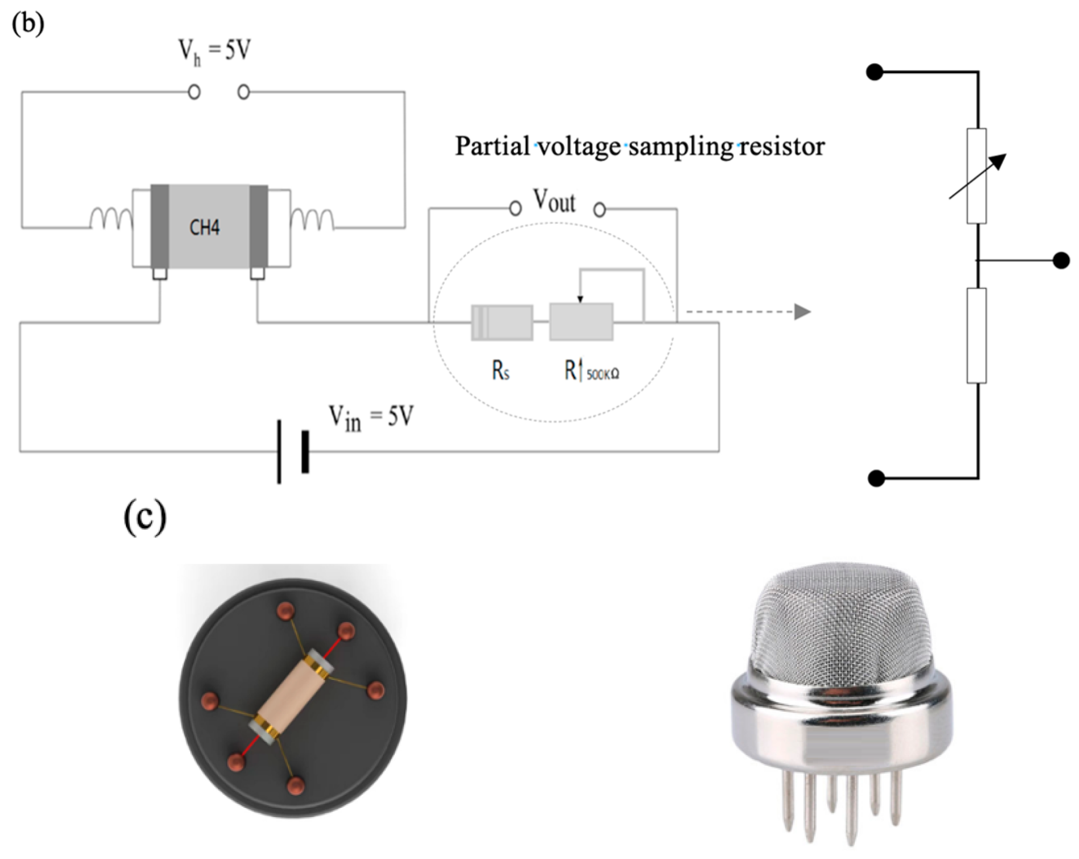
The dataset was acquired by our experimental system set of methane sensor arrays in this paper. Figure 4a shows the experimental system set of methane sensor arrays. The experimental system of the gas sensor array is mainly used in laboratory conditions to test and examine the sensitivity and temperature performance of the sensor array. When the external stress is loaded onto the sensor array through the experimental system, the stress value can be detected by the sensor in the system. When there is vibration, swing, air pressure change, or temperature change in the simulation, the vibration sensor, pitch sensor, air pressure sensor, and temperature sensor in the experimental system can detect the stress change value in real time. The fan in the experimental system can simulate a change in air flow movement, the heater can simulate a change in temperature, and the humidifier can simulate a change in humidity. These change factors are applied to the sensor array, and the environmental adaptability of the sensor array can be assessed.
In practice, the system will be tested and trained to qualify the array of sensors, mounted on an underwater vehicle for use. However, the experimental system in this paper only plays the role of training and evaluating the sensors.
A program-controlled relay, potentiometer, and voltage device are included in the fault transmitter. The communication module is employed to realize data transmission and two-way communication with the host computer. The main part of the test system is integrated into the host computer to bring down control commands and receive all sorts of temperature, humidity, sway, vibration, air pressure, and gas concentration detections from the communication module, to collect the output signals of sensor arrays to extract feature information, and to process fault data. The structure of the sensor signal detection circuit is displayed in Figure 4b. In addition, Figure 4c shows the cylinder core structure of an MQ-6 gas sensor. All the programs are operated under a 2.8-GHz Intel CPU with 16 GB of RAM running Windows 10.
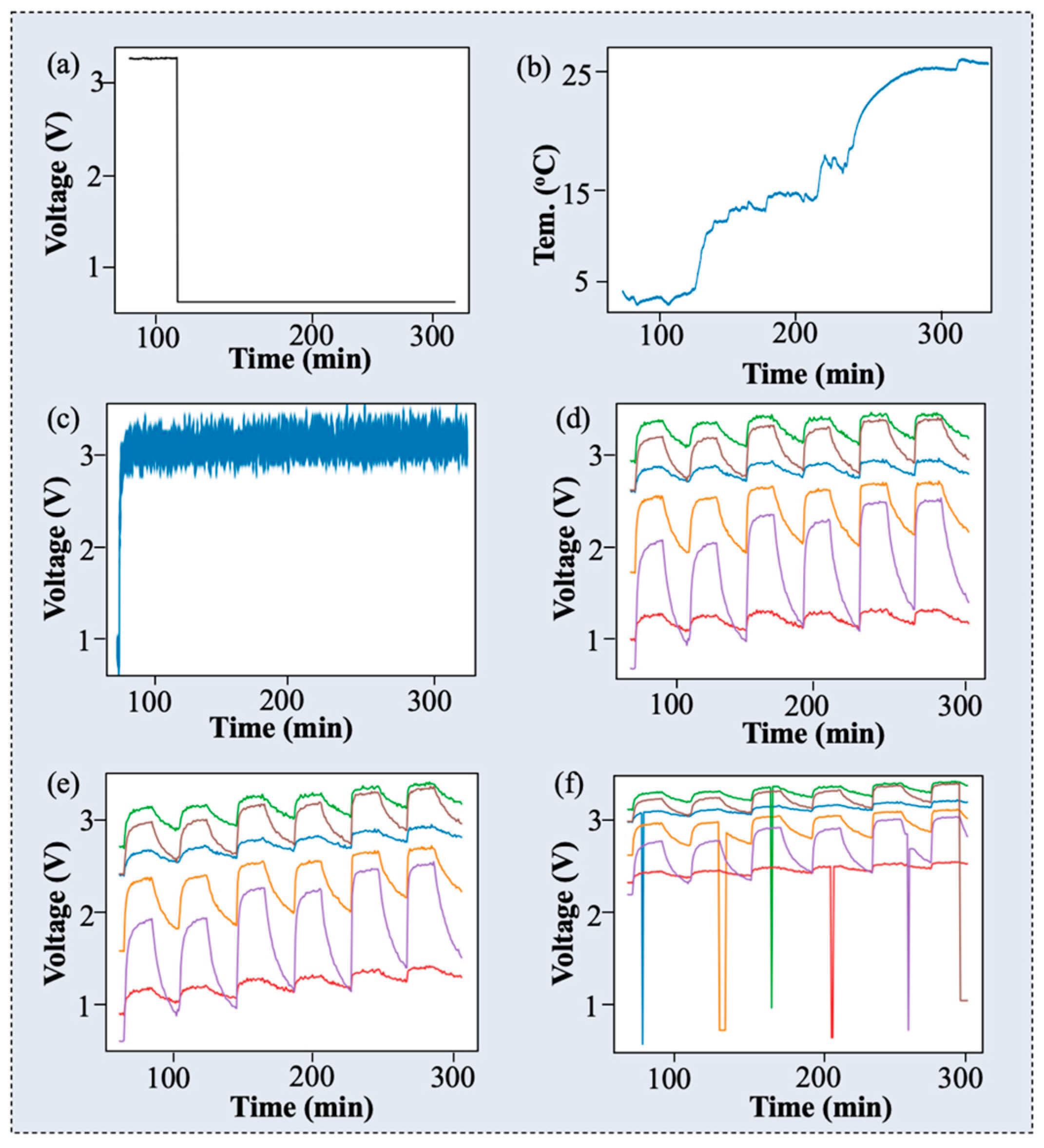
In the anomaly detection task, the split curve and final curve are shown in Figure 5. These curves’ information includes methane sensor array data in Figure 5d, anomaly point information in Figure 5a, temperature information in Figure 5b, and simulated vibration and swing information from the engine in Figure 5c that is operating in the deep-sea environment. To evaluate the efficiency of the methods of anomaly detection, the heating wire disconnection irregularity (HWDI) type of anomaly data and simulated anomaly points were added to the original data, which is likely the situation before the sensor array fault diagnosis. Assuming no existence of a single fault in the methane sensor array under actual conditions, various anomaly points in each pattern at a different time were added to simulate the situation under actual conditions. The proposed six-sensor array anomaly data are as changeable as real situations, which can be a counterpart to the anomaly detection task in reality. The temperature, sway, and noise in the background were also added to simulate the complicated environment in Figure 5e. In total, 1800 points of methane sensor array data were combined with 18 simulated anomaly points to constitute the type of unbalanced data that were obtained in Figure 5f. The probability density and correlation of normal and anomaly methane sensor array data are shown in Figures S2 and S3. As can be seen from Figure S2, the probability distribution of normal data and anomaly data is different, which also indicates that the data are very different, and it is difficult to verify the model. As can be seen from Figure S2, the correlation of anomaly data is significantly lower than that of normal data. This is determined by the data itself, and this low correlation requires a higher detection ability of the model.

3.2. Experimental Flowchart of Anomaly Warning Detection Systems

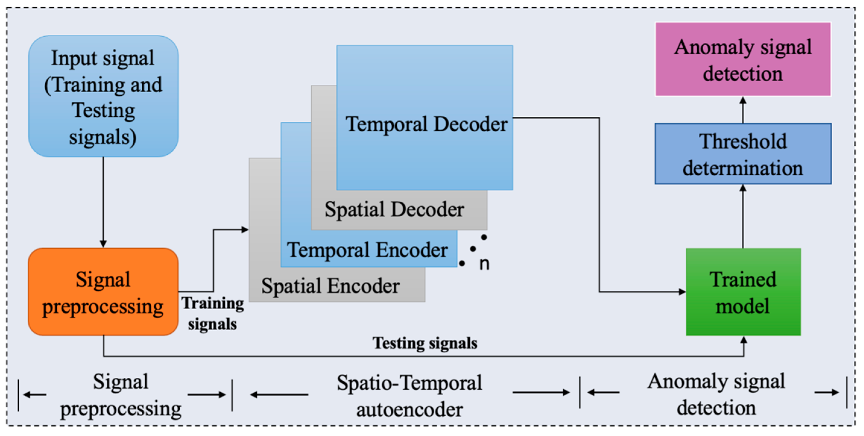
The ESST transformer model is considered to be a smart model for anomaly detection according to the multi-sensor data for changeable operating circumstances. An experimental diagram of the proposed method is shown in Figure 6, and the detection process is as follows.
Step 1: In the training part, normal methane data were reconstructed, the time and spatial information of the data were learned through the ESST transformer, and the loss of training was minimized.
Step 2: In the data transfer part, the trained model parameters were decreased with normal data information and transferred to an anomaly dataset.
Step 3: In the anomaly detection part, the loss value of the output of anomaly data was calculated by using the proposed adaptive threshold method. The anomaly sensor and time were then found.

3.3. Validation of Anomaly Detection Method and Inference

3.3.1. Anomaly Detection Evaluation Metrics

The evaluation metrics of anomaly detection methods are described in this segment. The precision rate in (10), recall rate in (11), F measure in (12), and accuracy rate (Acc.) in (13) are adopted to evaluate the anomaly detection.
P r e c i s i o n = T P T P + F P
R e c a l l = T P T P + F N
F 1   s c o r e = 1 + x 2 × P r e c i s i o n × R e c a l l α 2 × P r e c i s i o n × R e c a l l
A c c = T P + T N T P + T N + F P + F N
where TP, FP, and FN and TN, FP, and FN denote the true positive, false positive, and false negative rates of the samples. In particular, α = 1 is used in this paper.
The model performance is evaluated by the mean absolute error (MAE), mean squared error (MSE), and root mean squared error (RMSE) of true targets and predicted targets. The MAE, MSE, and RMSE are calculated by the following equations:
M A E = 1 n i = 1 n y _ t e s t y p r e
M S E = 1 n i = 1 n y _ t e s t y _ p r e 2
R M S E = 1 n i = 1 n y _ t e s t y _ p r e 2
where y_test and y_pre represent the true value and predicted value in the testing dataset, respectively. Moreover, n is the number of testing samples.

3.3.2. Results

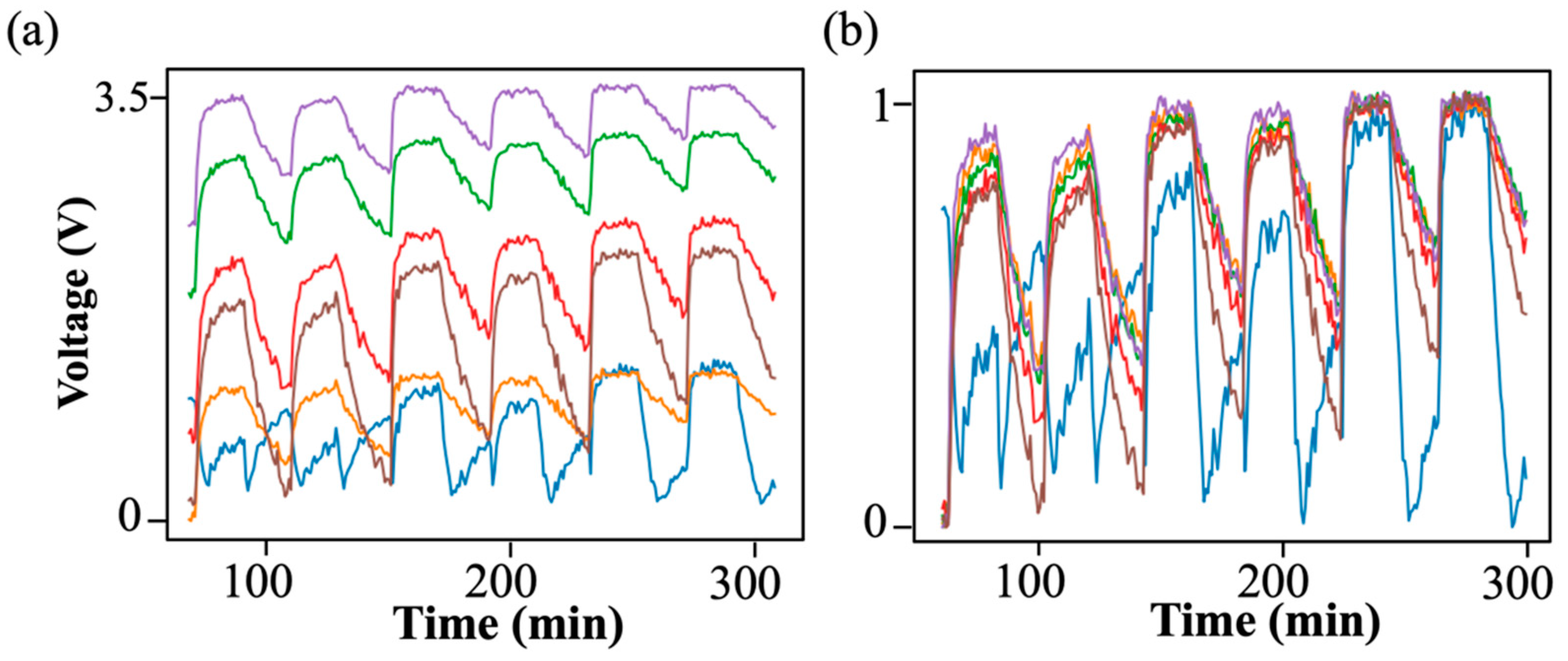
During training, 50 training iterations of the ESST transformer model were performed. The value of the batch size and the learning rate were set to 5 and 0.0001, which was the dynamic learning speed. As the training epochs were increased, however, the learning rates were dynamically reduced by 0.0005 every 10 epochs, in order to help the model to find the global optimal solutions more quickly. Reconstructed data results by the ESST trans. model are shown in Figure 7a,b. It can be seen that there is little difference between the reconstruction graph with (0,1) regularization in Figure 7b and the original graph in Figure 7a, which indicates that the model has learned the information of the sensor data and reconstructed it well.
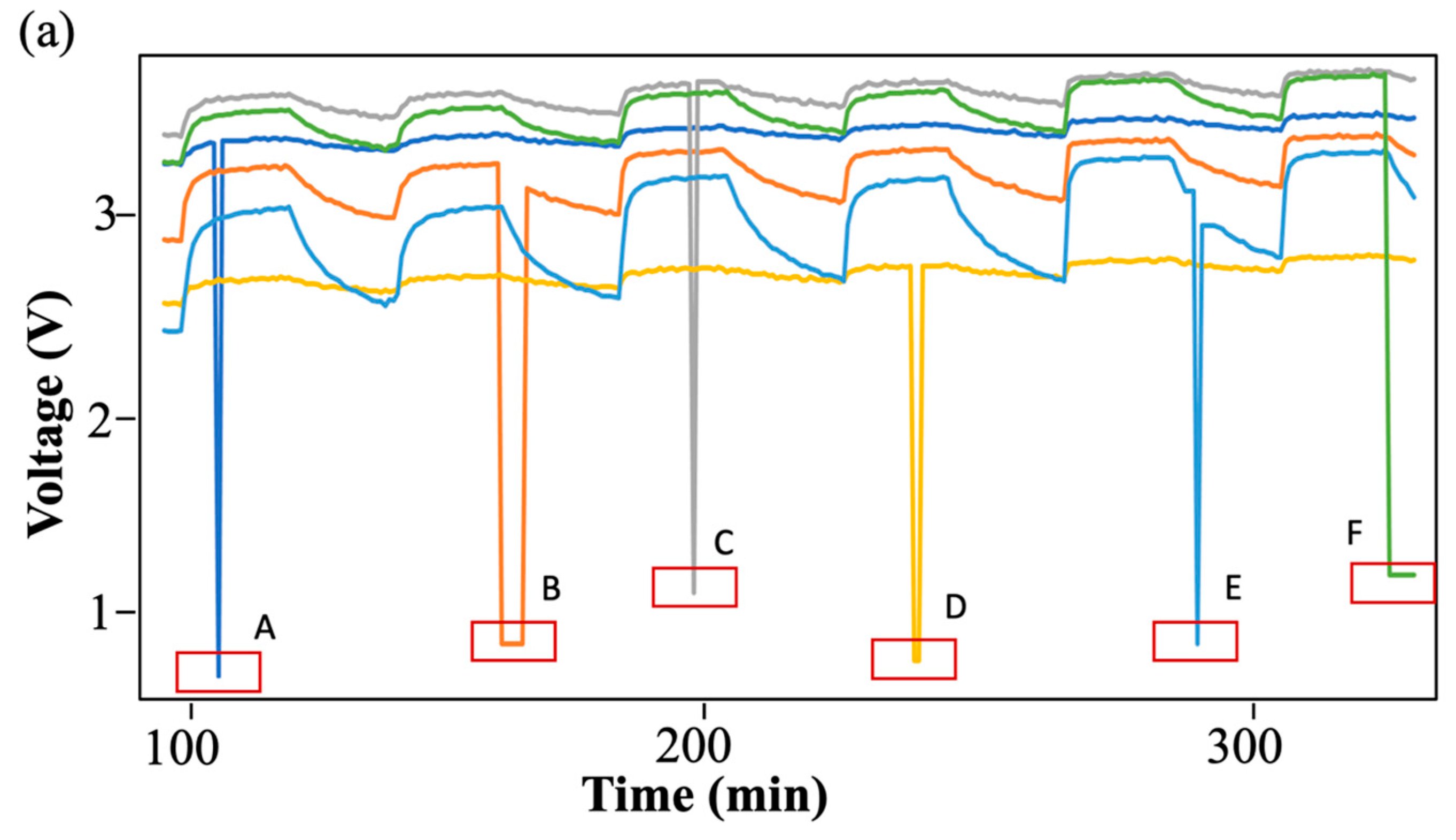
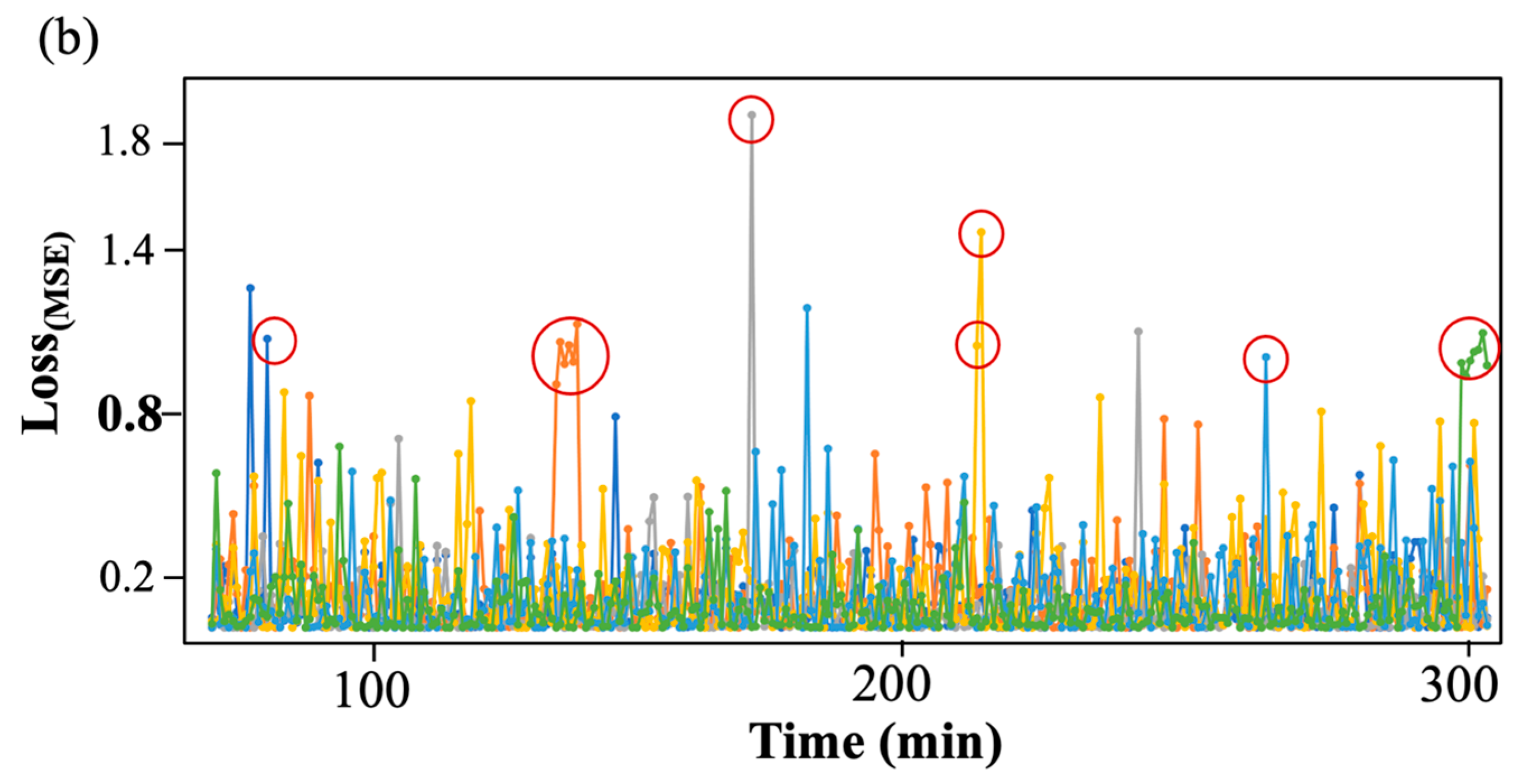
The anomaly detection result by the proposed model is marked with a red rectangle in Figure 8a, and the MSE loss of reconstructed anomaly data by the ESST trans. model with red circles is shown in Figure 8b. It is shown that the model can distinguish all anomaly data by manually setting the anomaly threshold to 0.8. It is shown that the MSE loss of the anomaly data was totally up to the threshold at 0.8, which shows that the model can all detect these anomaly data. In addition, the result for methane sensor array anomaly detection by the ESST trans. is presented in Table 2. As can be seen from Table 2, all six anomaly places have been detected by the ESST model, which is marked with a red circle in Figure 8b.
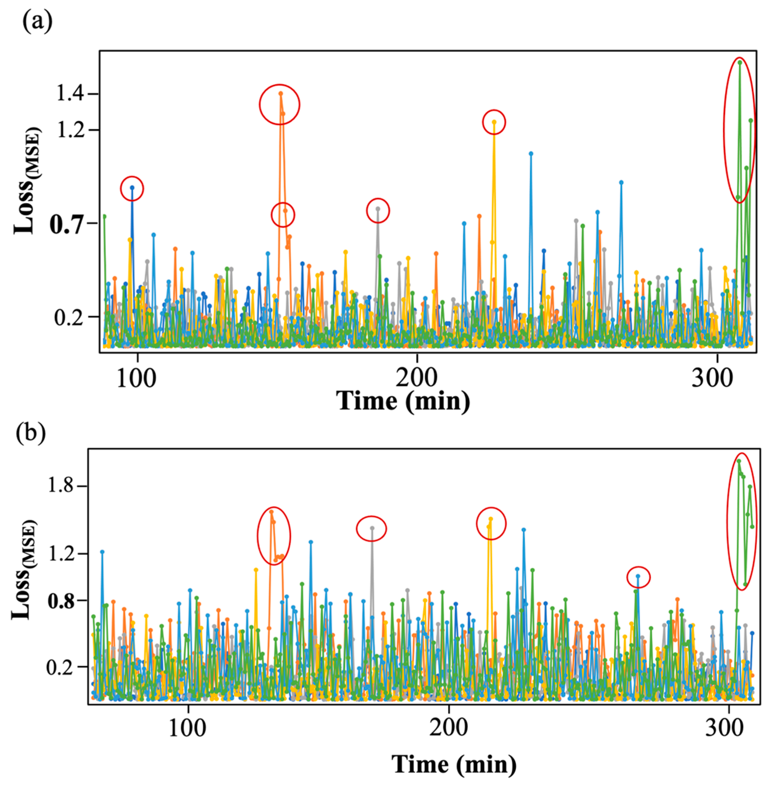
To validate the characteristics of the given method, other related approaches were chosen to evaluate the accuracy of anomaly detection. The comparative methods included the convolutional neural network autoencoder (CAE) and the long short-term memory autoencoder (LSTM_AE). The MSE loss of reconstructed anomaly data with the compared models is shown in Figure 9. It was shown that the compared models can only distinguish part of the anomaly data, which is more than threshold 0.7 and 0.8. It can be seen from Figure 9a that 10 anomaly points (marked as red circles) are detected, which is greater than the threshold value of 0.7. It can be seen from Figure 9b that 14 anomaly points (marked as red circles) are detected, which is greater than the threshold of 0.8. The MSE loss values of the trained data and normal data training process with the comparison models are shown in Figure S4. From Figure S4, it can be seen that the gradient value of the training loss when trained by different models is different, which indicates that the models used in the experiment are different.
A comparison between the MSE loss value of the trained original data and anomaly data is displayed in Table 3. It can be seen that the MSE loss of abnormal points is remarkably higher than the data value of normal points.
The anomaly detection metrics of the three methods are shown in Table 4. It can be clearly seen that the LSTM_AE method has the lowest training time of 520 s, and the proposed model has a higher F1 score of 0.92 as well as higher anomaly accuracy, respectively. Due to the parallel computing ability of the transformer, the training time is in the middle, and the proposed model has a higher F1 score and high precision, which represents the anomaly detection accuracy.

3.4. Attention Visualization for Anomaly Detection in Training Process

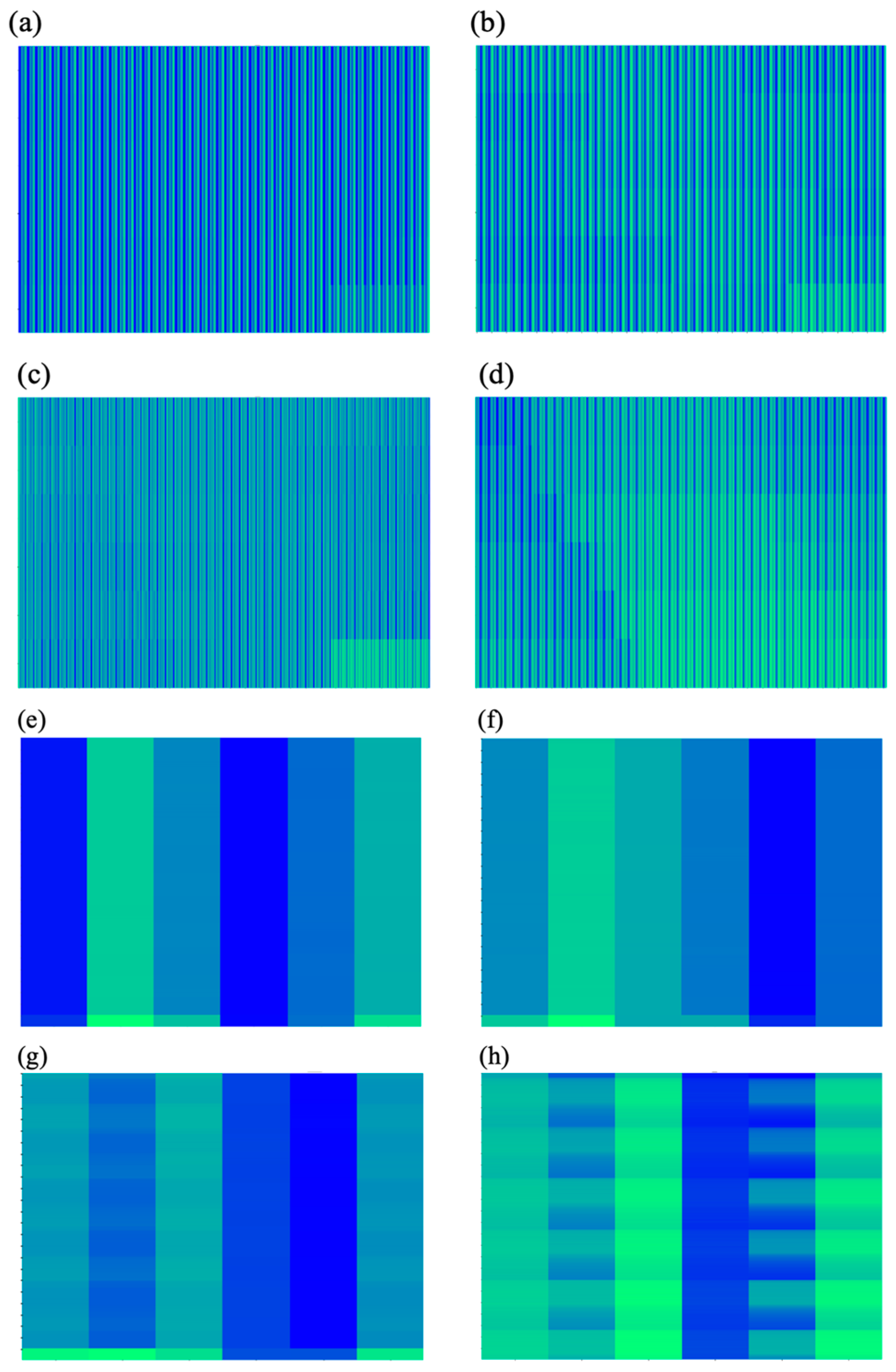
Figure 10 shows a thermodynamic diagrammatic sketch of the attention mechanism during the training process of anomaly detection. Thermodynamic diagrams of attention after training 5 epochs, 10 epochs, 30 epochs, and 50 epochs are presented, respectively. To reflect the visualization of the attention mechanism in the training, the visualization results were divided into two parts, which are presented in forms (300,6) and (6,300), respectively, and four attention process graphs in each form are presented.
From (300,6) and (6,300), we can observe that with the increase in epochs, the attention visualization map of the proposed model gradually tends to the final sensor array data’s map. This trend proves that the model has convergence.

3.5. Contrast of Time Complexity with Different Models

Time complexity was reduced with several related efforts listed in Table 5. Three parallel models are adopted, i.e., Dai et al. (2019) [47], Child et al. (2019) [48], and Kitaev et al. (2020) [49]. It can be seen that the ESST trans. The model minimizes the time complexity to O (n). The model used fixed patterns or combinations of fixed patterns to remove the time complexity to O (n). The effect of the model is fancy, without any performance degradation.

3.6. Discussion

The ESST transformer model proposed in this paper is an end-to-end structure that can learn the information of spatio-temporal characteristics and solve the problem of outlier detection by explaining the three processes of sparse mask, sparse spatio-temporal attention mechanism, and anomaly warning system. ESST enables the transformer network to automatically focus on other locations related to the current position when processing different locations in the sequence, giving different weights to these locations, and assigning greater weights to important features. At runtime, the ESST transformer model can dynamically adjust the weights according to the context, helping the transformer model to better focus on important information when processing sequence data, thus improving the outlier detection capability. This was proven through a comparison of CAE, LSTM_AE, and ESST trans. The F1 score of the algorithm is 0.92, and the accuracy of outlier detection is 85.71%. This shows that the constructed ESST transformer model has good advancement and applicability in solving the problem of methane sensor array outlier detection.
The interpretability method shows the characteristics of the middle layer of the network, which is used to understand and explain the features learned by the model. The explainable sparse spatio-temporal feature attention mechanism proposed in this paper can effectively improve the accuracy of outlier detection of the network. In order to better understand and explain the training process of abnormal detection of the attention mechanism, the interpretability method is used to show the process of the spatial attention mechanism. The idea of this method is to add an interpretable sparse spatio-temporal feature attention mechanism to the transformer model structure and follow the network to complete the training. The feature map of the attention mechanism is obtained and enlarged to form a heat map to understand and explain the process of the attention mechanism. The experimental results show the heat map of attention training for 5 epochs, 10 epochs, 30 epochs, and 50 epochs. In order to reflect the visualization of the attention mechanism process in training, the interpretable results are presented in the form of (300,6) and (6,300), and each form has four attention process graphs. With the increase in epochs, the attention process graph gradually tends to the final sensor array data graph, showing more accurate feature expression of the target, strong guidance abilities for feature learning of the model, and more comprehensive coverage of the main area of the target, so that it can more accurately identify the sensor outlier target. This trend proves that the interpretable sparse spatio-temporal feature attention mechanism model has excellent convergence.

4. Conclusions

Sensor outliers refer to individual values in the detection data that seriously deviate from the observed values of other objects. There is an essential difference between abnormal data and incomplete data generated by interference, noise, and error, and the generation of abnormal data is related to the failure of the functional components of the sensor itself. The generation of abnormal sensor data sometimes represents potential laws and trends, which is intrinsically related to the occurrence and failure laws of sensor faults. In most practical scenarios, the exception data themselves are unlabeled and difficult to identify.
In view of the importance of outlier detection, this paper proposes a deep learning method based on an interpretable sparse spatio-temporal transformer model for anomaly data detection of an underwater methane remote-sensing sensor array. Firstly, the classical self-attention mechanism is improved. Sparse blocks are established based on the graph sparsification method and physical response characteristics of the sensor array data, and the time complexity is reduced to O (n) through interpretable sparse blocks. Secondly, the traditional self-attention block is improved, and the spatio-temporal enhanced attention block is established. The spatio-temporal attention block can automatically capture the spatio-temporal characteristics of gas sensor array signals at different time scales through the query matrix and automatically capture the temporal characteristics including temperature information through the key matrix, which is used for outlier detection of methane sensor array data. Finally, the anomaly detection threshold technology is set as a data-driven early warning system, and the data-driven alert return mechanism contains the alert threshold associated with the physical disturbance information. This is an unsupervised learning method, which can eliminate the influence on the sensor array from environmental interference signals such as ambient temperature, vibration, and sway and improve the accuracy of anomaly detection. In order to realize a data-driven early warning system, the proposed model is a data-based transfer unsupervised learning method, which has low data acquisition cost and is more suitable for industry promotion and application.
The results show that the interpretable sparse space-time converter improves the anomaly detection behavior of the underwater methane remote-sensing sensor array. The F1 score of the proposed model is 0.92, which is better than other reconstruction models (Convolutional_AE, LSTM_AE) such as convolution autoencoder (0.81) and long short-term memory autoencoder (0.66). Moreover, our work is superior in terms of O (n) time complexity only, compared to the O (n2) time complexity of the original transformer model. The results verify that the ESST model provides an idea for the anomaly detection of an underwater methane remote-sensing sensor array, and it can be used for outlier detection. It has the advantages of low computational complexity, high speed, and high precision in the online application of an underwater methane remote-sensing sensor array.

5. Future Work

This paper mainly uses the generated model to address the issue of anomaly detection. However, although the calculation of the proposed model is reduced to O (n), there are still cases in which the calculation of the model is too complicated. We will increase more interpreted blocks of the model in order to reduce the complexity. These blocks will increase the interpretability of the model and reduce unnecessary calculations. The accuracy of anomaly detection will remain the same as in the ESST model.
(1). The generation of abnormal values in the methane sensor array is related to the functional composition of the composed gas sensors. The semiconductor methane gas sensor used in this study is a suspended structure; hence, its ability to withstand objective environmental factors is weak. Abnormal and sudden changes in environmental conditions such as mechanical shock and external vibration can cause measurement anomalies in gas sensor arrays. Therefore, improving the integrated structure design of sensors and adopting more advanced thin-film integrated sensors can effectively enhance the overall resistance of sensor arrays to environmental interference, which will be an effective way to reduce the occurrence of outliers in sensor array operation.
(2). The generation of abnormal values in the methane sensor array is related to the performance of the gas sensor signal acquisition circuit. The signal acquisition circuit used in this study is a Wheatstone bridge circuit with DC power supply, which has insufficient processing ability for high-frequency signals, impulse signals, electromagnetic pulse signals, and other interference signals. Once these interference signals appear, they can also cause abnormal values in the sensor array. Therefore, designing more advanced low-pass filter circuits that can suppress high-frequency noise and improve the performance of sensor signal acquisition circuits will effectively enhance the sensor array’s ability to resist external interference signals. This is an effective way to reduce the occurrence of outliers in sensor array operation.
(3). To improve the credibility of the transformer model and make model decisions more transparent, it is necessary to strengthen the visualization of feature importance and decision tree visualization research and to deeply explore association rules, which will help the interpretability of the model. The transformer model uses an attention mechanism to handle global dependencies between inputs and outputs. However, an attention module that requires a large amount of matrix operations leads to the complexity and computational time cost of the model. Studying advanced variants of multi-head self-attention, improving the spatial resolution of attention mechanisms, and enhancing the generalization ability of models are effective ways to improve the efficiency and accuracy of anomaly detection.

Supplementary Materials

The following supporting information can be downloaded at: https://www.mdpi.com/article/10.3390/rs16132415/s1.

Author Contributions

Conceptualization, K.Z., W.N. and Y.Z.; formal analysis, T.W.; methodology, W.J.; writing—original draft preparation, K.Z.; writing—review and editing, M.Z. and Z.Y.; funding acquisition, M.Z. and Z.Y. All authors have read and agreed to the published version of the manuscript.

Funding

This work was supported by the National Key Research and Development Program of China (2022YFC3104700), the National Natural Science Foundation of China (62371299, 62301314, and 62101329), and the China Postdoctoral Science Foundation (2023M732198). We also acknowledge analysis support from the Instrumental Analysis Center of Shanghai Jiao Tong University and the Center for Advanced Electronic Materials and Devices of Shanghai Jiao Tong University. The computations in this paper were run on the π 2.0 cluster supported by the Center for High-Performance Computing at Shanghai Jiao Tong University.

Data Availability Statement

For privacy reasons, given the sensitive nature of the data, the aggregated data analyzed in this study will not be publicly disclosed but might be available on request from the corresponding author.

Conflicts of Interest

The authors declare no conflicts of interest. The funders had no role in the design of the study; in the collection, analyses, or interpretation of data; in the writing of the manuscript; or in the decision to publish the results.

References

  1. Irina, T.; Ilya, F.; Aleksandr, S. Mapping Onshore CH4 Seeps in Western Siberian Floodplains Using Convolutional Neural Network. Remote Sens. 2022, 14, 2611. [Google Scholar] [CrossRef]
  2. Ying, W.; Xu, G.; Hong, Z. Characteristics and emissions of isoprene and other non-methane hydrocarbons in the Northwest Pacific Ocean and responses to atmospheric aerosol deposition. Sci. Total Environ. 2023, 10, 162808. [Google Scholar]
  3. Liu, S.; Xue, M.; Cui, X.; Peng, W. A review on the methane emission detection during offshore natural gas hydrate production. Front. Energy Res. 2023, 11, 12607–12617. [Google Scholar] [CrossRef]
  4. Itziar, I.; Javier, G.; Daniel, Z. Satellites Detect a Methane Ultra-emission Event from an Offshore Platform in the Gulf of Mexico. Environ. Sci. Technol. Lett. 2022, 9, 520–525. [Google Scholar]
  5. Ian, B.; Vassilis, K.; Andrew, R. Simultaneous high-precision, high-frequency measurements of methane and nitrous oxide in surface seawater by cavity ring-down spectroscopy. Front. Mar. Sci. 2023, 10, 186–195. [Google Scholar]
  6. Zhang, X.; Zhang, M.; Bu, L.; Fan, Z.; Mubarak, A. Simulation and Error Analysis of Methane Detection Globally Using Spaceborne IPDA Lidar. Remote Sens. 2023, 15, 3239. [Google Scholar] [CrossRef]
  7. Wei, K.; Thor, S. A review of gas hydrate nucleation theories and growth models. J. Nat. Gas Sci. Eng. 2019, 61, 169–196. [Google Scholar]
  8. Gajanan, K.; Ranjith, P.G. Advances in research and developments on natural gas hydrate extraction with gas exchange. Renewable and Sustainable Energy Reviews. Renew. Sustain. Energy Rev. 2024, 190, 114045–114055. [Google Scholar] [CrossRef]
  9. Zhao, H.; Zhang, Y. Detection Method for Submarine Oil Pipeline Leakage under Complex Sea Conditions by Unmanned Underwater Vehicle. J. Coast. Res. 2020, 97, 122–130. [Google Scholar] [CrossRef]
  10. Liu, C.; Liao, Y.; Wang, S.; Li, Y. Quantifying leakage and dispersion behaviors for sub-sea natural gas pipelines. Ocean Eng. 2020, 216, 108–117. [Google Scholar] [CrossRef]
  11. Li, Z.; Ju, W.; Nicholas, N. Spatiotemporal Variability of Global Atmospheric Methane Observed from Two Decades of Satellite Hyperspectral Infrared Sounders. Remote Sens. 2023, 15, 2992. [Google Scholar] [CrossRef]
  12. Wang, P.; Wang, X.R.; Guo, Y.; Gerasimov, V.; Prokopenko, M.; Fillon, O.; Haustein, K.; Rowan, G. Anomaly detection in coal-mining sensor data, report 2: Feasibility study and demonstration. Tech. Rep. CSIRO 2007, 18, 21–30. [Google Scholar]
  13. Song, Z.; Liu, Z. Anomaly detection method of industrial control system based on behavior model. Comput. Secur. 2019, 84, 166–172. [Google Scholar]
  14. Jiang, W.; Liao, X. Anomaly event detection with semi-supervised sparse topic model. Neural Comput. Appl. 2018, 31, 3–10. [Google Scholar]
  15. Schmidl, S.; Wenig, P. Anomaly detection in time series: A comprehensive evaluation. Proc. VLDB Endow. 2022, 15, 1779–1797. [Google Scholar] [CrossRef]
  16. Bi, W.; Zao, M. Outlier detection based on Gaussian process with application to industrial processes. Appl. Soft Comput. 2019, 76, 505–510. [Google Scholar]
  17. Xi, Z.; Yi, H. Variational LSTM enhanced anomaly detection for industrial big data. IEEE Trans. Ind. Inf. 2020, 20, 87–94. [Google Scholar]
  18. Cheng, H.; Tan, P.N.; Potter, C.; Klooster, S. A robust graph-based algorithm for detection and characterization of anomalies in noisy multivariate time series. ICDM 2008, 4, 123–132. [Google Scholar]
  19. Bi, Z.; Qi, S. Deep autoencoding gaussian mixture model for unsupervised anomaly detection. In Proceedings of the International Conference on Learning Representations, Vancouver, BC, Canada, 30 April–3 May 2018; Volume 10, pp. 302–311. [Google Scholar]
  20. Lorenzo, B.; Rota, C. Natural gas consumption forecasting for anomaly detection. Expert Syst. Appl. 2016, 62, 190–201. [Google Scholar]
  21. Ma, S.; Nagpal, R. Macro programming through Bayesian networks: Distributed inference and anomaly detection. IEEE Int. Conf. Pervasive Comput. Commun. 2007, 5, 87–96. [Google Scholar]
  22. Markus, M.; Noah, D. LOF: Identifying density-based local outliers. In Proceedings of the 2000 ACM SIGMOD International Conference on Management of Data, Dallas, TX, USA, 16–18 May 2000; Volume 5, pp. 302–311. [Google Scholar]
  23. Mohammed, B.; Sindre, B. Unsupervised Anomaly Detection for IoT-Based Multivariate Time Series: Existing Solutions, Performance Analysis and Future Directions. Sensors 2023, 23, 2844. [Google Scholar] [CrossRef] [PubMed]
  24. Yan, S.; Shao, H.; Xiao, Y.; Liu, B.; Wan, J. Hybrid robust convolutional autoencoder for unsupervised anomaly detection of machine tools under noises. Robot. Comput.-Integr. Manuf. 2023, 79, 102441. [Google Scholar] [CrossRef]
  25. Malhotra, A.; Pankaj, D. Long short term memory networks for anomaly detection in time series. Comput. Intell. Mach. Learn. 2015, 10, 600–620. [Google Scholar]
  26. Yadav, M.; Malhotra, H. Ode-augmented training improves anomaly detection in sensor data from machines. NIPS Time Ser. Workshop. 2015, 20, 405–411. [Google Scholar]
  27. Chandola, V.; Banerjee, A. Anomaly detection: A survey. ACM Comput. Surv. 2009, 41, 15–22. [Google Scholar] [CrossRef]
  28. Bedeuro, K.; Mohsen, A. A Comparative Study of Time Series Anomaly Detection Models for Industrial Control Systems. Sensors 2023, 23, 1310. [Google Scholar] [CrossRef] [PubMed]
  29. Ting, K.; Bing, Y. Outlier detection for time series with recurrent autoencoder ensembles. IJCAI 2019, 20, 2725–2732. [Google Scholar]
  30. Buitinck, L.; Louppe, G. API design for machine learning software: Experiences from the scikit-learn project. ICLR 2013, 14, 14–20. [Google Scholar]
  31. Dark, P.; Yong, H. A multimodal anomaly detector for robot-assisted feeding using an LSTM-based variational autoencoder. IEEE Robot. Autom. Lett. 2018, 3, 1544–1551. [Google Scholar]
  32. An, J.; Cho, S. Variational autoencoder based anomaly detection using reconstruction probability. Spec. Lect. 2015, 30, 302–311. [Google Scholar]
  33. Pong, M.; Amakrishnan, K. LSTM-based encoder-decoder for multi-sensor anomaly detection. CVPR 2016, 10, 1267–1273. [Google Scholar]
  34. Chen, X.; Deng, L.; Huang, F.; Zhang, C.; Zhang, Z.; Zhao, Y.; Zheng, K. DAEMON: Unsupervised Anomaly Detection and Interpretation for Multivariate Time Series. In Proceedings of the 2021 IEEE 37th International Conference on Data Engineering (ICDE), Chania, Greece, 19–22 April 2021; Volume 20, pp. 3000–3020. [Google Scholar]
  35. Raghavendra, C.; Sanjay, C. Deep learning for anomaly detection: A survey. arXiv 2019, arXiv:1901.03407. [Google Scholar]
  36. Yasuhiro, I.; Kengo, T.; Yuusuke, N. Estimation of dimensions contributing to detected anomalies with variational autoencoders. AAAI 2019, 14, 104–111. [Google Scholar]
  37. Li, D.; Chen, D.; Jin, B.; Shi, L.; Goh, J.; Ng, S.K. Mad-Gan: Multivariate anomaly detection for time series data with generative adversarial networks. In Proceedings of the International Conference on Artificial Neural Networks, Gran Canaria, Spain, 12–14 June 2019; Springer: Berlin/Heidelberg, Germany, 2019; Volume 21, pp. 703–716. [Google Scholar]
  38. Zhang, C.; Song, D.; Chen, Y.; Feng, X.; Lumezanu, C.; Cheng, W.; Ni, J.; Zong, B.; Chen, H.; Chawla, N.V. A deep neural network for unsupervised anomaly detection and diagnosis in multivariate time series data. AAAI 2019, 33, 1409–1416. [Google Scholar] [CrossRef]
  39. Julien, A.; Pietro, M. USAD: Un-Supervised anomaly detection on multivariate time series. In Proceedings of the 26th ACM SIGKDD International Conference on Knowledge Discovery & Data Mining, Virtual Event, 24 August 2020; Volume 20, pp. 3395–3404. [Google Scholar]
  40. Deng, A.; Hooi, B. Graph neural network-based anomaly detection in multivariate time series. AAAI 2021, 5, 403–411. [Google Scholar] [CrossRef]
  41. Li, L.; Yan, J.; Wang, H.; Jin, Y. Anomaly detection of time series with smoothness-inducing sequential variational auto-encoder. IEEE Trans. Neural Netw. Learn. Syst. 2021, 32, 201–211. [Google Scholar] [CrossRef] [PubMed]
  42. Li, Z.; Zhao, Y.; Han, J.; Su, Y.; Jiao, R.; Wen, X.; Pei, D. Multivariate time series anomaly detection and interpretation using hierarchical inter-metric and temporal embedding. KDD 2021, 3, 3220–3230. [Google Scholar]
  43. Dzmitry, B.; Kyunghyun, C. Neural machine translation by jointly learning to align and translate. arXiv 2015, arXiv:1409.0473. [Google Scholar]
  44. Ashish, V.; Noam, S. Attention is all you need. NIPS 2017, 3, 6000–6010. [Google Scholar]
  45. Luong, T.; Hieu, P. Effective approaches to attention-based neural machine translation. In Proceedings of the 2015 Conference on Empirical Methods in Natural Language Processing, Lisbon, Portugal, 17–21 September 2015; Volume 15, pp. 1412–1421. [Google Scholar]
  46. Iz, B.; Matthew, P.; Arman, C. Longformer: The Long-Document Transformer. arXiv 2020, arXiv:2004.05150. [Google Scholar]
  47. Dai, Z.; Yang, Z.; Yang, Y.; Carbonell, J.; Le, Q.V.; Salakhutdinov, R. Transformer-XL: Attentive language models beyond a fixed-length context. arXiv 2019, arXiv:1901.02860. [Google Scholar]
  48. Rewon, C.; Scott, G. Generating long sequences with sparse transformers. arXiv 2019, arXiv:1904.10509. [Google Scholar]
  49. Nikita, K.; Lukasz, K. Reformer: The efficient transformer. In Proceedings of the International Conference on Learning Representations, Addis Ababa, Ethiopia, 30 April 2020; Volume 4, pp. 148–156. [Google Scholar]
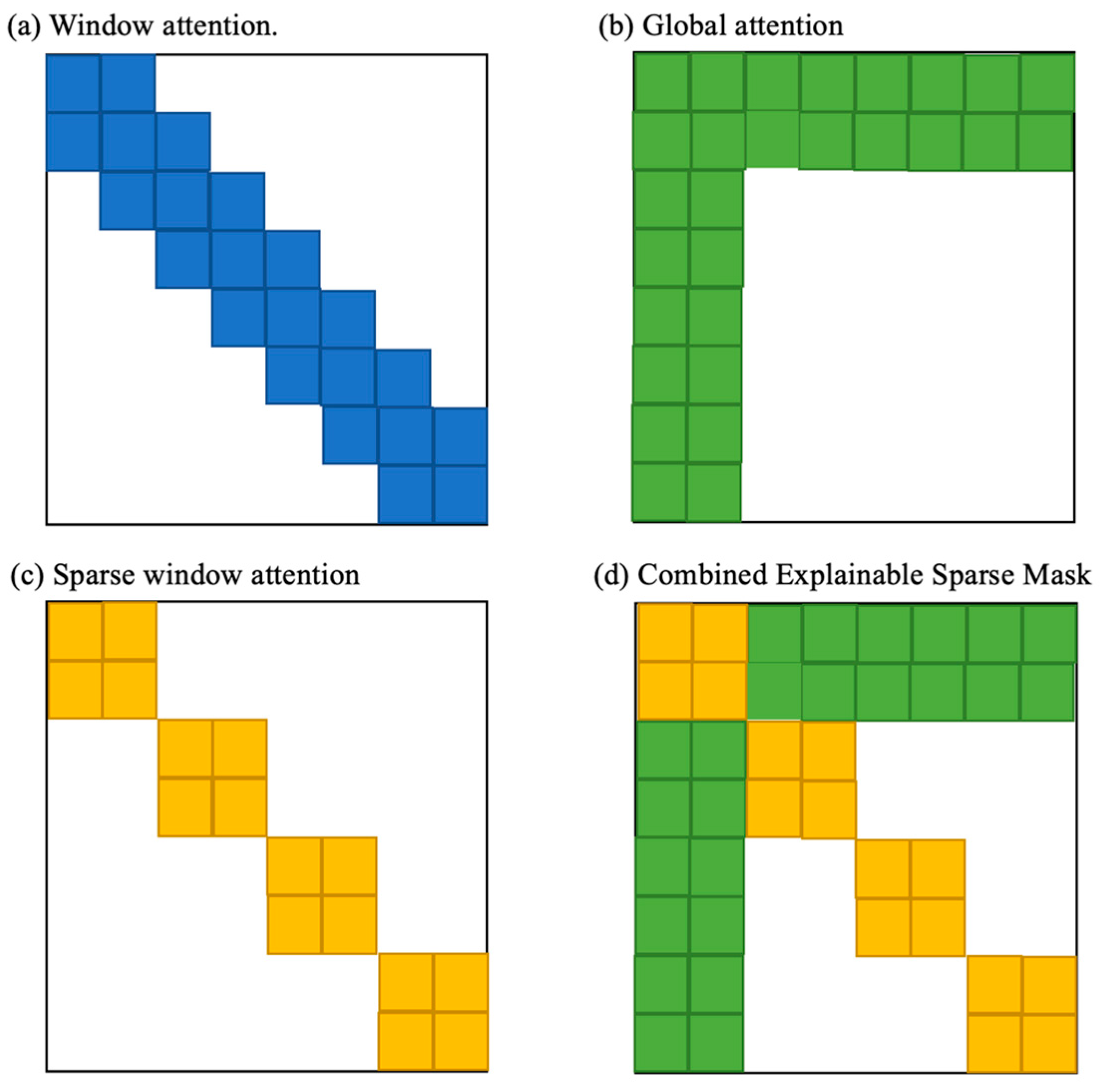
Figure 1. Building blocks of the mask mechanism adopted by the ESST transformer. White color indicates the absence of a mask. (a) Sliding window mask of w = 3; (b) global attention of g = 2; (c) sparse window attention with T = 1/6; (d) combined explainable sparse mask.
Remotesensing 16 02415 g001
Figure 2. Traditional self-attention module and ESST attention mechanism.
Remotesensing 16 02415 g002
Figure 3. Signal reconstruction flowchart by generative ESST trans.
Remotesensing 16 02415 g003
Figure 4. Experimental setup using the gas sensor array: (a) experimental system diagram, (b) gas sensor circuit diagram, (c) methane gas sensor.
Remotesensing 16 02415 g004aRemotesensing 16 02415 g004b
Figure 5. Different kinds of methane sensor single curves. Different colored lines represent each methane sensors (MQ-6). (a) HWDI anomaly point signal. (b) Temperature curve. (c) Noise and sway curve. (d) Original methane sensor array data. (e) The combined normal curve. (f) The combined anomaly curve.
Remotesensing 16 02415 g005
Figure 6. Flowchart of anomaly warning detection systems.
Remotesensing 16 02415 g006
Figure 7. Reconstructed data results by ESST trans. model. Different colored lines represent each methane sensors (MQ-6): (a) original methane data reconstructed; (b) reconstructed methane data regularized from 0 to 1.
Remotesensing 16 02415 g007
Figure 8. Anomaly detection system results by ESST trans. model. Different colored lines represent each methane sensors (MQ-6) and its MSE loss. (a) Anomaly data of methane sensor array. The letters A–F indicate six anomaly places, which mark with a red rectangle in (a). (b) MSE loss of reconstruction anomaly data by ESST trans. model.
Remotesensing 16 02415 g008aRemotesensing 16 02415 g008b
Figure 9. MSE loss of reconstructed anomaly data by (a) LSTM-AE, (b) CAE. Different colored lines represent each MSE loss of methane sensors (MQ-6), and the anomaly points are marked as red circles.
Remotesensing 16 02415 g009
Figure 10. Attention visualization for normal data reconstruction task in two forms, (6,300) and (300,6), respectively. (a) Epoch 5, MSE 2.15; (b) Epoch 10, MSE 1.08; (c) Epoch 30, MSE 0.95; (d) Epoch 50, MSE 0.40; (e) Epoch 5, MSE 2.42; (f) Epoch 10, MSE 1.21; (g) Epoch 30, MSE 0.82; (h) Epoch 50, MSE 0.42.
Remotesensing 16 02415 g010
Table 1. Different kinds of the ESST trans. models.
Layer KindLayer TypeLayer DescriptionDropoutMask Number
1dff, dk, dv128, 32, 32no-
2dmodel16no-
3Multi-attentionHead = 2yes2
4EncoderN = 4yes2
5DecoderN = 4yes2
Table 2. Results on methane sensor array anomaly detection by ESST trans. method.
LocationEstimated ClassesActual
CleanOutlier
Sen.1 (14)01Outlier
Sen.2 (82–87)01Outlier
Sen.3 (128)01Outlier
Sen.4 (181–182)01Outlier
Sen.5 (249)01Outlier
Sen.6 (295–301)01Outlier
Table 3. MSE loss for the trained original data and anomaly data.
LocationSensor Data (V)ESST (MSE)LSTM-AE (MSE)CAE (MSE)
OriginalAnormalCleanOutliersCleanOutliersCleanOutliers
Sen.1 (14) 3.140.01 0.25 0.98 0.05 0.84 0.22 0.36
Sen.2 (82–87) 2.960.2 0.05 0.95 0.2 0.69 0.2 1.26
Sen.3 (128) 3.470.5 0.01 1.73 0.03 0.84 0.29 1.23
Sen.4 (181–182) 2.410.1 0.15 1.12 0.2 0.55 0.01 1.25
Sen.5 (249) 2.750.2 0.01 0.92 0.51 0.16 0.01 0.89
Sen.6 (295–301) 3.470.6 0.1 0.93 0.12 0.75 0.1 1.6
Table 4. Anomaly detection results by different methods under industrial conditions.
ModelsTraining Time
(s)
F1 Score
(0~1)
Recall
(%)
Precision
(%)
Anomaly Acc.
(%)
CAE6000.8194.4470.8394.44
LSTM_AE5200.6655.5676.9255.56
ESST Trans.5600.9210085.71100
Table 5. Summary of efficient transformer models.
Model/PaperComplexityDecodeClass
Trans.-XL (Dai et al., 2019) [47]O (n2) RC
Sparse Trans. (Child et al., 2019) [48] O   ( n n ) FP
Reformer (Kitaev et al., 2020) [49]O (n·log n) LP
ESST Trans.O (n) FP
Ps: FP, fixed patterns or combinations of fixed patterns; LP, learnable pattern; RC, recurrence.
Disclaimer/Publisher’s Note: The statements, opinions and data contained in all publications are solely those of the individual author(s) and contributor(s) and not of MDPI and/or the editor(s). MDPI and/or the editor(s) disclaim responsibility for any injury to people or property resulting from any ideas, methods, instructions or products referred to in the content.