Abstract
Reliable and spatially explicit information on global crop yield has paramount implications for food security and agricultural sustainability. However, most previous yield estimates are either coarse-resolution in both space and time or are based on limited studied areas. Here, we developed a transferable approach to estimate 4 km global wheat yields and provide the related product from 1982 to 2020 (GlobalWheatYield4km). A spectra–phenology integration method was firstly proposed to identify spatial distributions of spring and winter wheat, followed by choosing the optimal yield prediction model at 4 km grid scale, with openly accessible data, including subnational-level census data covering ~11,000 political units. Finally, the optimal models were transferred at both spatial and temporal scales to obtain a consistent yield dataset product. The results showed that GlobalWheatYield4km captured 82% of yield variations with an RMSE of 619.8 kg/ha, indicating good temporal consistency (r and nRMSE ranging from 0.4 to 0.8 and 13.7% to 37.9%) with the observed yields across all subnational regions covering 40 years. In addition, our dataset generally had a higher accuracy (R2 = 0.71) as compared with the Spatial Production Allocation Model (SPAM) (R2 = 0.49). The method proposed for the global yield estimate would be applicable to other crops and other areas during other years, and our GlobalWheatYield4km dataset will play important roles in agro-ecosystem modeling and climate impact and adaptation assessment over larger spatial extents.
1. Introduction
Approximately 800 million people worldwide suffered from undernourishment in 2020 [1]. Sustainable Development Goal (SDG) 2 is dedicated to eradicating hunger and all forms of malnutrition by 2030 and achieving food security [2]. However, the goal of eliminating hunger might remain elusive even by 2050 due to climate variability, extreme weather events, and global crises such as the COVID-19 pandemic and the current Russia–Ukraine war [3]. Climate change is projected to force an additional 72 million people to face hunger risks in 2050, and the COVID-19 pandemic is estimated to have led to 83–132 million more undernourished people in 2020 [3,4]. In these contexts, global food production needs to increase by at least 70% to feed the unprecedented population growth of up to 10 billion by 2050 [5,6]. To better inform a series of agricultural resource allocation and food security decisions, timely and accurate information on crop yield at a global scale is of paramount significance [7,8,9,10].
There are two mainstream methods of crop yield prediction, that is, process-based crop models and statistical methods [11,12,13,14,15,16]. Crop models can dynamically simulate crop physiological processes, including development, growth, and grain formation processes [17,18,19,20,21]. Despite incorporating diverse physiological mechanisms, crop models are highly dependent on substantial data inputs and massive computations [22]. On the other hand, statistical models often relate crop yields to diverse predictor variables (e.g., vegetation indices and climatic variables) and calibrate the empirical relationships based on measurements [23]. The superiority of statistical models lies in their simplicity and reduced requirement for extensive inputs; however, they are particularly vulnerable to co-linearity problems and noise of inputs [24]. Fortunately, machine learning (ML) provides an innovative alternative to statistical modeling and can address the nonlinear relationships between the predictor variables and crop yield, demonstrating superior performance in many applications [25,26,27,28]. For instance, Kang et al. (2020) proved that more advanced ML models achieved better accuracy in estimating county-level maize yield [29]. Emerging breakthroughs in algorithms such as deep learning (DL) approaches have accomplished more accurate crop yield estimation [30,31]. For example, the long short-term memory (LSTM) model adopts a recurrent neural network structure that can recognize sequential information for long time periods and capture sophisticated nonlinear relationships. Jiang et al. (2020) found that LSTM outperformed the RF model in estimating county-level corn yields in the United States [32]. The superior performance of LSTM over two ML approaches was further proved during the prediction of wheat yield in the Guanzhong Plain by Tian et al. (2021) (e.g., support vector machines) [33].
Previous studies using ML and DL methods focused on very limited areas rather than global scales. It is well recognized that a global spatially explicit crop yield dataset has important implications for large-scale agricultural system modeling and climate change impact assessments [34,35,36]. Although a few studies have filled such data gaps, there is still room for significant development. For example, a 10 km global dataset of harvested area and yield was firstly generated for 175 crops circa 2000 [37], followed by the Global Agro-ecological Zones (GAEZ) datasets in 2000 and 2010 [38], Spatial Production Allocation Model (SPAM) at 5-arcmin resolution for three years (2000, 2005, and 2010) [39], and the latest data proposed by Grogan et al. (2022) with a resolution of 5 min for 2015 [40]. However, these four publicly accessible products only cover 1~3 years, hampering related studies on investigating the long-term impacts of climate change on yields [41,42]. Iizumi et al. (2020) developed a global dataset of historical yields (GDHY) for staple crops at a spatial resolution of 0.5° by integrating agricultural census data and remote sensing [43]. GDHY covers a longer period, but its spatial resolution is relatively coarse. Moreover, these yield datasets were established based on crop distribution maps generated by a downscaling method rather than accurate satellite-derived maps, which might result in misestimated yield and inaccurate assessments of climate change impacts [44]. Therefore, it is urgent to acquire the global gridded yield dataset with a higher resolution and a longer time span based on the accurate spatial distribution of harvesting areas.
In this study, by integrating multi-source data (e.g., remote sensing, climate, soil data, and subnational-level census data) and data-driven methods, we aim to (1) propose a transferable method to accurately estimate global crop yield; (2) compare the performance of two ML and DL models in predicting gridded yields; and (3) choose the optimal models to generate global wheat yield datasets. The resultant dataset with 4 km spatial resolution will benefit the investigation of spatiotemporal patterns of crop production, assessment of climate change impacts and modeling of crop growth processes over large spatial extents.
2. Materials and Methods
2.1. Study Area
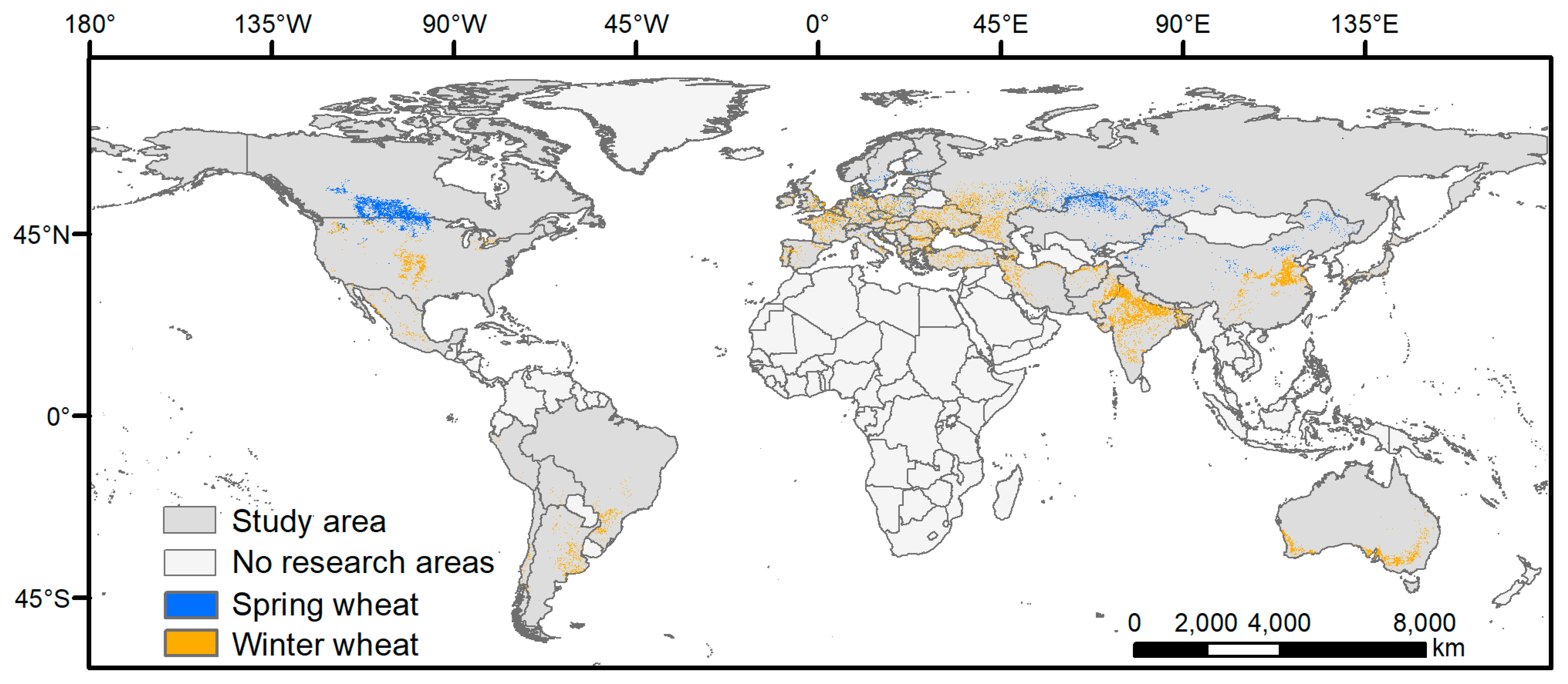
The study area contains the main wheat-planting countries (54) in the world, covering ~92% of the total harvested area and ~93% of the total production (Figure 1) [45]. We compiled the abundant subnational-level census data in the countries, with diverse climatic conditions and cropping systems. Winter wheat dominates the majority (>75%) of global wheat harvesting area, while areas of spring wheat <25% (primarily in the Northern Hemisphere high latitude areas such as the United States, the Russian Federation, and Canada) [46,47].
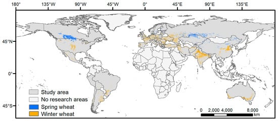
Figure 1.
The spatial distribution of spring and winter wheat covering 54 countries globally.
2.2. Data
2.2.1. Remote Sensing Data
We acquired the global daily 0.05° Normalized Difference Vegetation Index (NDVI) data during 1981–2021 derived from the Advanced Very High-Resolution Radiometer (AVHRR) sensor on the Google Earth Engine (GEE) platform. The data were generated using eight NOAA polar orbiting satellites (i.e., NOAA-7, -9, -11, -14, -16, -17, -18, and -19) and VIIRS for two time periods before and after 2014. The main strength of AVHRR NDVI lies in its longest time coverage, which can be used to derive predictors for yield prediction [48]. In addition, the 8 d composite Global Land Surface Satellite (GLASS) Leaf Area Index (LAI) at 1 km spatial resolution from 2005 to 2015 was used to capture phenological information on different crops, and the Global Food Security-support Analysis Data (GFSAD) 1 km Crop Mask product (GFSAD1KCM) was utilized as a cropland mask. The GLASS LAI was retrieved using general regression neural networks with multiple inputs (http://glass-product.bnu.edu.cn/?pid=3&c=1, accessed on 19 June 2024), with the specific advantages of being spatiotemporally continuous without gaps and having higher accuracy than other datasets [49,50]. GFSAD1KCM provides the global cropland extent for the nominal year 2010 and is produced based on four inputs with the highest accuracy of 85% [51]. Moreover, the annual dataset of the 1 km wheat harvesting area (named ChinaCropArea1km) in China during 2000–2015 was used [52].
2.2.2. Wheat Harvesting Area and Yield
The subnational-level census data on harvested area (unit: ha), production (unit: ton), and yield (unit: kg/ha) were collected from ~11,000 administrative units in the 54 countries, with the longest time coverage spanning from 1981 to 2020. Yield is calculated as production divided by harvested area. Overall, 97% of data came from administrative unit level 2 (ADM2) and 3 (ADM3). For the European Union, the data were collected at NUTS-2 level. The temporal coverage differs across the study area (Table S1). We eliminated outliers of census data with values +/−2 standard deviations from the average.
2.2.3. Environmental Data
Meteorological information was obtained from high-spatial resolution (1/24°, ~4 km) monthly TerraClimate datasets [53]. The climate variables used for this analysis were maximum temperature (Tmin), minimum temperatures (Tmax), precipitation (Pre), vapor pressure (Vap), vapor pressure deficit (Vpd), reference evapotranspiration (Petref), soil moisture (Soil), Palmer drought severity index (Pdsi), and downward surface shortwave radiation (Srad) from 1981 to 2021. In addition, soil properties were derived from the Harmonized World Soil Database (HWSD) at 0.00833° (~1 km), involving the bulk density, organic carbon content, pH, gravel, clay, and sand and silt fraction for the topsoil (0–30 cm) [54] (see Table 1).

Table 1.
Summarization for information on each country across the study area.
2.3. Methods
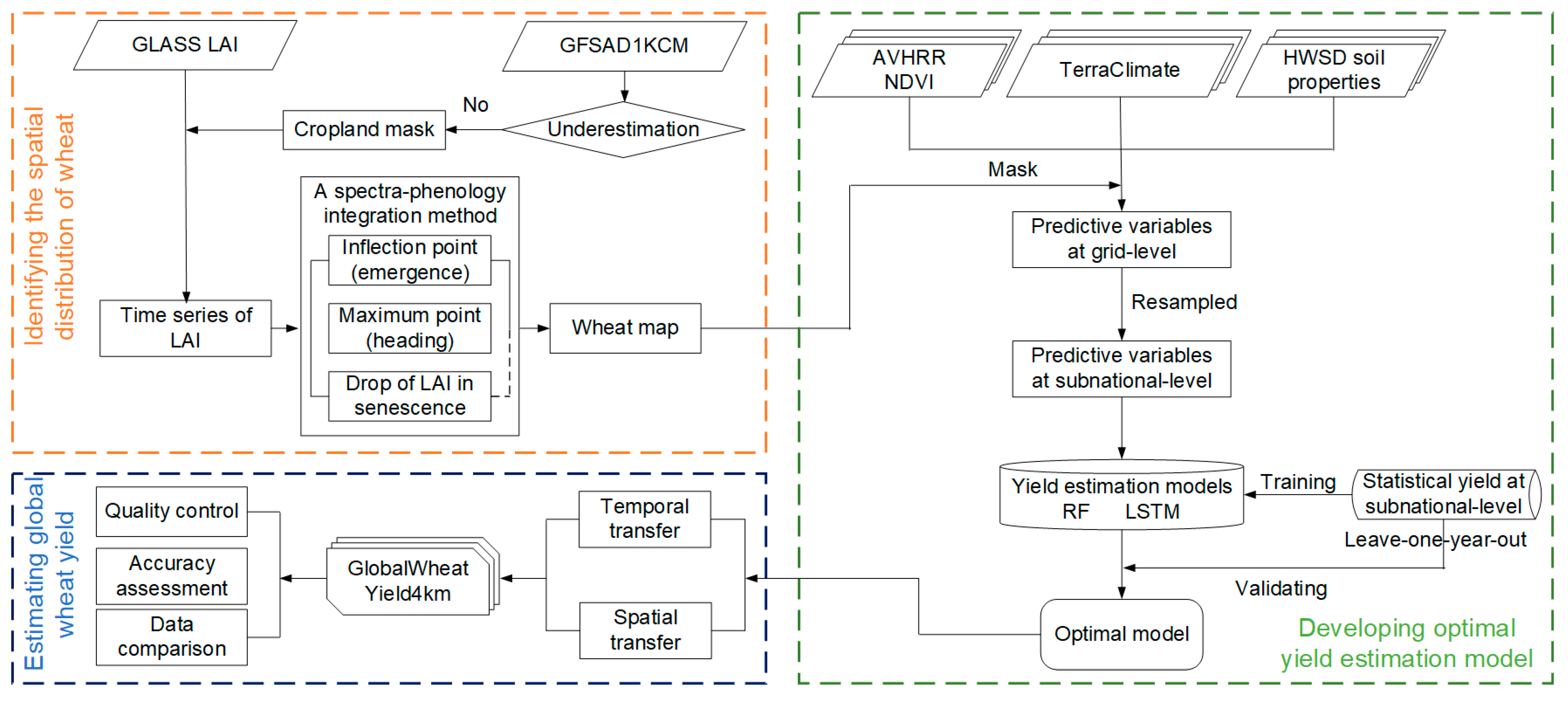
We applied the Global Wheat Production Mapping System (GWPMS) framework developed by Luo et al. (2022) with two aspects of improvement (Figure 2) [44]. We conducted the study according to the following: (1) mapping the harvesting area of spring and winter wheat by a spectra–phenology integration algorithm; (2) comparing the performances of two ML and DL approaches in predicting gridded yield, (3) generating the GlobalWheatYield4km dataset using the optimal model, and (4) evaluating the accuracy and uncertainty of the dataset.
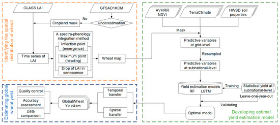
Figure 2.
Flow chart of spatiotemporal transferable method to estimate global wheat yields.
2.3.1. Identifying the Spatial Distribution of Wheat
Phenology information plays a paramount role in large-scale crop mapping [52,55,56]. The phenological dates of winter wheat are earlier than summer crops and spring wheat and are later than some winter crops such as winter barley [44,57]. For example, the sowing date of winter wheat often occurred in autumn, while that of summer crops and spring wheat was concentrated in spring, leading to earlier timing of heading and maturity. In addition, the duration of the growth period of winter wheat is generally longer. Spring wheat can also be differentiated from other summer crops as its phenological phases occur earlier. Therefore, we developed a wheat detection algorithm that formalized these features in rules to automatically detect the harvest areas of spring and winter wheat [44]. Here, we modified the algorithm and mapped the spatial distribution of wheat as following steps.
First, we compared the cropland map derived from the GFSAD1KCM with census data to determine whether to use it as a cropland mask; that is, the mask was utilized only when the GFSAD1KCM-derived areas matched with (or were larger than) census data.
Second, we used the Savitzky–Golay (S-G) filter method to remove the noise from the GLASS LAI composites for each pixel. This method has shown good performance for smoothing time series [58,59,60].
Lastly, we utilized the algorithm to detect annual spatial distribution of spring and winter wheat during 2006–2014. Generally, three specific characteristics should be recognized concurrently, namely, the green-up of winter wheat or emergence of spring wheat, heading, and crop senescence. Specifically, the green-up/emergence of winter/spring wheat was regarded as an inflection point after which the first derivative increased for three adjacent images. The heading date was identified as the maximum point within a restricted time window obtained from existing work regarding wheat phenology, with the LAI value exceeding a certain threshold (LAImax). Moreover, crop senescence signal was detected as a sharp decline in the LAI (LAI decreased by more than LAIdec%) during a 40-day time period. In addition, we modified the algorithm when applying it to some regions where winter wheat was not a dominant crop (e.g., Mexico, Bolivia, and Peru) or grown in rotation with other crops (e.g., Argentina and Brazil in South America, India and Pakistan in Southeast Asia, and China). For example, the rule for the heading and senescence phase was loosened or even eliminated when the signal was weak due to the mixed pixel issues or the short duration of the interval between the maturity date of winter wheat and the planting date of the second crop (Table S2).
2.3.2. Estimating Gridded Yield Using Data-Driven Models
We first compared the predictive performance of two commonly used ML and DL approaches, i.e., the Random Forest (RF) and LSTM models. The RF model combines a set of decision trees that are constructed from a random subset of data [61]. Each tree is trained separately on these samples, and the remaining data are called out of bag (OOB) samples and can be used to validate the RF model. In this study, we used the Python scikit-learn library to develop the RF regression model. The number of decision trees (n_estimators), the minimum number of samples required to be at a leaf node (min_samples_leaf), and the number of features (max_features) were selected for tuning. The LSTM network consists of a framework of a recurrent neural network (RNN) and memory gate structure, demonstrating superior performance in coping with sequential data and capturing the nonlinear and cumulative relationships between crop yield and meteorological factors [32,62]. The model consists of an input layer, one or more LSTM layers, and an output layer. The LSTM layers are composed of LSTM cells, in which information is forgotten or outputted decided by three gates. Batch normalization was firstly implemented for all the input data. The transient data (i.e., NDVI and climate data) were dealt with via two LSTM layers that have 200 hidden units, whereas the non-sequential data (i.e., soil properties) were appended to the final LSTM layer and then fully connected to the output layer. In addition, a rectified linear unit (ReLU) activation function was used for all the layers. The model was run for 2000 maximum iterations with a mini-batch size of 500, and RMSprop was used to optimize hyperparameters with a learning rate of 0.001. The LSTM network for estimating gridded yield was performed on TensorFlow (GPU version 2.0). Keras, a deep learning library, was applied for developing the LSTM model.
Here, we first resampled the gridded input data (i.e., NDVI, climate, and soil data) into 4 km and unified NDVI and climate data into monthly time steps by the maximum value synthesis and monthly mean method, individually. The time series of monthly NDVI composites were further gap-filled by a moving median method [63], which replaced the missing data with the median composite of three adjacent values (i.e., preceding, current, and subsequent values). Then, we derived an integrated wheat map to represent reliable spatial distribution over a long-term period on the basis of the grids with cultivation for at least 5 years during 2006–2014. Finally, all input data were averaged on the subnational scale after being masked by wheat cultivation pixels. These processes were performed on the Google Earth Engine (GEE) platform.
We implemented the “leave-one-year-out” method to examine performance of the ML and DL models, that is, one-year data were used for testing and the data of the remaining years for training. More specifically, each model was first trained separately by excluding one year in the data. For instance, the temporal extent of county-level statistics for the United States was from 1982 to 2016. If two models were trained with the data for the years 1982–1999 and 2001–2016, then they were validated using the data of 2000. The best hyperparameters were determined with the ten-fold cross-validated coefficient of determination (R2). Then, the optimized models were used to estimate gridded yield for the excluded year. Finally, the resultant yields were aggregated to the corresponding ADM level and were compared with census data for the excluded year. The R2 and root mean square error (RMSE) were calculated to validate estimates’ accuracy. The whole process was repeated 20 times, and the mean R2 and RMSE were used to compare the performance of the two data-driven models. Note that the evaluation metric of the RF model performance was the R2 and RMSE of the OOB validation (i.e., OOB R2 and RMSE).
The RF and LSTM models were generally constructed for each country; however, their predicted performance was poor in some countries (e.g., Kazakhstan) due to the limited statistical data. To improve the accuracy of the yield dataset and lengthen its time coverage, we first combined the census data of some countries together to train the model and spatially transferred it to estimate gridded yields. For example, we only collected observed yields of Kazakhstan for the years 2014–2020. Since the growing season of spring wheat was identical in the Russian Federation and Kazakhstan, their data were integrated to feed into the model, and the yield maps were ultimately generated from 1995 to 2020. Similar treatment was conducted for all European countries, as well as Afghanistan and Iran (Table S3). In addition, we applied the pre-trained model to other years where observed yields are unavailable, aiming at generating a spatiotemporally continuous yield dataset.
2.3.3. Uncertainty Analysis
To provide the uncertainty of GlobalWheatYield4km, we spatialized the normalized RMSE (nRMSE) to depict the spatial patterns of uncertainty. More specifically, we first calculated the nRMSE of the yield between the GlobalWheatYield4km-derived estimates and the observed data in each subnational unit. Then, the nRMSE value was allocated to the centroid of each subnational unit, and the kriging interpolation method was used to map the spatial distribution of uncertainty, which was masked by wheat cultivation pixels.
2.3.4. Comparison with Other Global Yield Datasets
We compared our gridded yield estimates with a prevalent product (i.e., SPAM) using census data to demonstrate the reliability of our dataset. These two datasets could be directly compared as they were both generated using census data. More specifically, we calculated the R2 and RMSE between the observed yield and the estimates of SPAM or GlobalWheatYield4km in 2000, 2005, and 2010. Since the crop yield of SPAM was the nominal value for three adjacent years centered on 2000, 2005, and 2010, the averages of observed yields in the corresponding years (e.g., the averages of 1999, 2000, and 2001 match SPAM 2000) were used.
3. Results
3.1. Assessing Accuracy of Wheat Distribution Maps
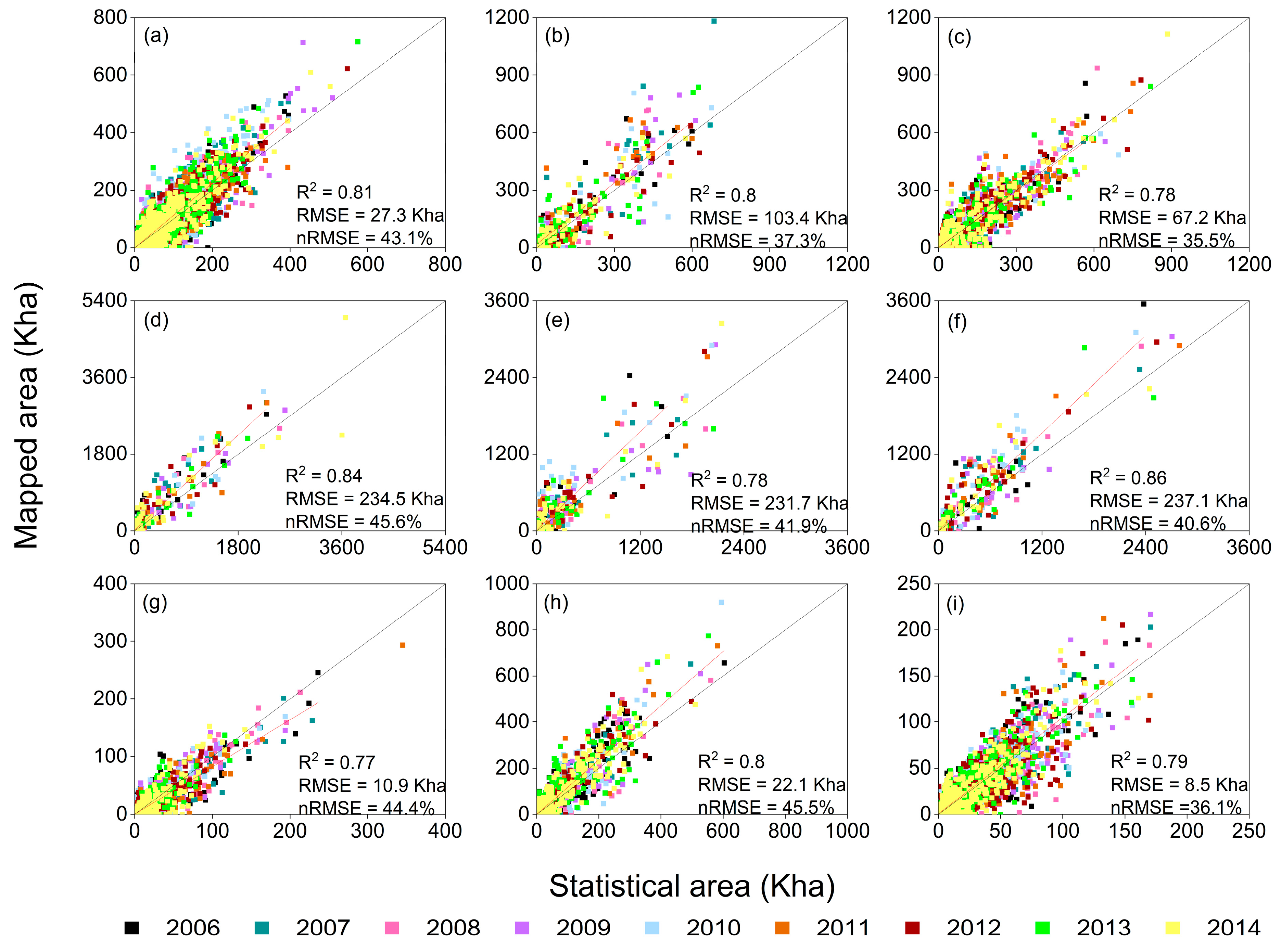
To illustrate the reliability of the wheat distribution maps, we validated them with the subnational-level area. The estimated areas generally matched well with the observed area, with an R2 ranging from 0.65 to 0.89 (average: 0.8) and nRMSE ranging from 31.4% to 54.7% (average: 41.1%) (Figure 3, Table S4). The mapped areas were overestimated in the Russian Federation, Kazakhstan, Australia, Canada, and the United States, while they were underestimated in South America. A possible reason for the overestimation could be the difficulty of distinguishing spring wheat from other spring cereals such as spring barley because of their similar phenology. In addition, the wheat distribution maps showed the lowest accuracy in South America, with an R2 ranging from 0.65 to 0.82 and nRMSE ranging from 38.3% to 48.3%, which was ascribed to the mixed pixels and the larger uncertainties from remote sensing products. Overall, the comparisons showed the high consistency between the resultant maps and the census data, demonstrating that the derived maps were reliable for further yield prediction.
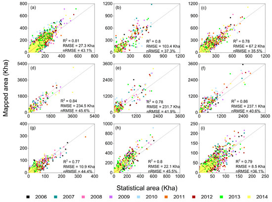
Figure 3.
Comparisons between mapped area by the spectra–phenology integration method and subnational-level data during 2006–2014. (a) South and East Asia, (b) Central Asia, (c) Europe, (d) spring wheat in the Russian Federation and Kazakhstan, (e) winter wheat in the Russian Federation, (f) Australia, (g) South America, (h) spring wheat in North America, and (i) winter wheat in North America.
Besides the above comparison of annual planting areas in the globe, we further selected the U.S. as an example to compare national spatial distribution in detail because of the popular CDL (Cropland Data Layer) products (Figure S1). The spatial distribution of our model matched well with CDL, with an R2 (RMSE) of 0.82 (6.2 Kha) and 0.81 (21.4 Kha) for winter and spring wheat, respectively. The higher accuracy (R2 > 0.80) together with lower RMSE further indicates the reliability of our maps derived from the spectra–phenology integration method.
3.2. Selecting the Optimal Model of Wheat Yield Estimates
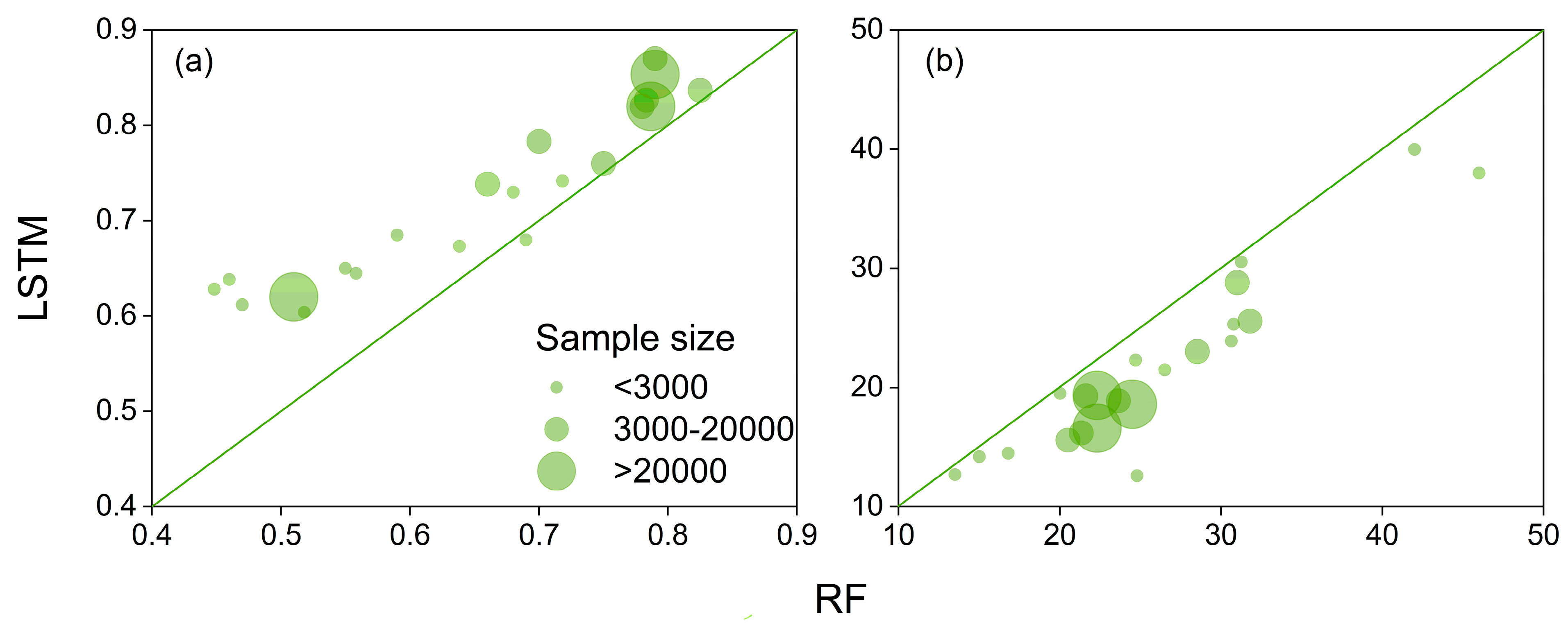
The performance of the RF and LSTM models in gridded yield prediction during 2006–2014 for each region/country is shown in Figure 4. Generally, the LSTM model outperformed the RF model, with an average R2 (nRMSE) of 0.72 (13.1%) and 0.64 (16.2%), respectively. More specifically, LSTM achieved the highest accuracy in the United States, Europe, China, India, and Pakistan (R2 > 0.8, nRMSE < 20%) while the RF model showed comparable performance (R2 of 0.7~0.82, nRMSE of 21%~29%), which was ascribed to the abundant training samples (>3000) (Table S3). However, compared to the better predictive performance of winter wheat in China and the United States, both the LSTM and RF model could capture less than 62% of yield variations in Brazil despite the sufficient statistical data. One possible reason was the many mixed pixels in Brazil with highly heterogeneous land cover types, consequently resulting in errors in aggregated predictor variables. The other was the larger uncertainties from remote sensing products, especially more frequent cloud contamination in Brazil. In addition, the RF model showed similar performance in Nepal (R2 = 0.69, nRMSE = 20%) as compared with LSTM (R2 = 0.68, nRMSE = 19.5%). A possible reason was that the training samples for Nepal were scarce, and the spatial variability of predictor variables and yield was relatively lower. Moreover, the LSTM models improved (decreased) R2 (nRMSE) by around 15% as compared with the RF model, especially in the Russian Federation, Ukraine, Bangladesh, Japan, Brazil, Peru, and Bolivia, with more improvements in R2 (nRMSE) ranging from 14% to 50%. The superior performance of LSTM was attributed to its powerful temporal learning capabilities that can capture nonlinear and cumulative relationships between yield and meteorological factors over long time periods.
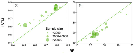
Figure 4.
Performance of the RF and LSTM models in yield estimation during 2006–2014 across all regions: (a) R2, (b) nRMSE (%).
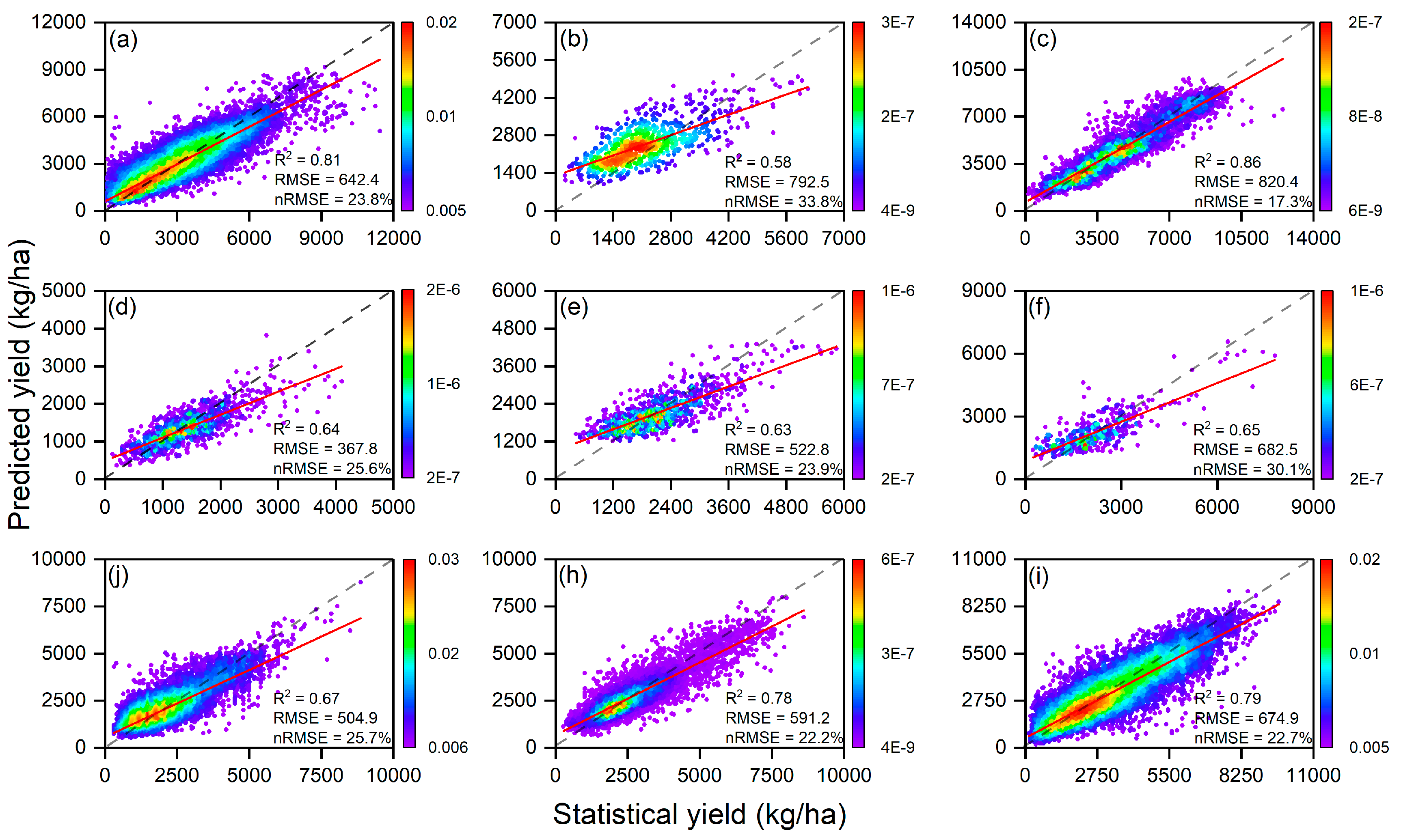
Therefore, the optimal LSTM model was implemented to predict global wheat yield at the grid scale. The out-of-sample performance was evaluated over the subnational level, and the time period is same as that of observed yields (Table S1). More specifically, the model was recursively trained using all data after leaving one year for testing, and the gridded-yield estimates were aggregated to the subnational level and validated by the remaining year. Overall, the predicted yield agreed well with the census data as they were closely and consistently distributed around the 1:1 line, with an R2 of 0.56~0.86, RMSE of 123.2~911.3 kg/ha, and nRMSE of 13.8~33.8% (Figure 5 and Figure S2). The overall R2 of GlobalWheatYield4km was 0.82 across all subnational regions and years, with the RMSE and nRMSE values of 619.8 kg/ha and 23.5%, respectively. The highest R2 was found in Bangladesh (R2 = 0.86, nRMSE = 14.9%) and Europe (R2 = 0.86, nRMSE = 17.3%), followed by China, Chile, Pakistan, India, Canada, and the United States (R2 of 0.77~0.82). By contrast, the lowest R2 was found in Japan (R2 = 0.56, nRMSE = 20.6%), Afghanistan, and Iran (R2 = 0.58, nRMSE = 33.8%), which might be caused by the lower wheat cultivation or insufficient observed yields.
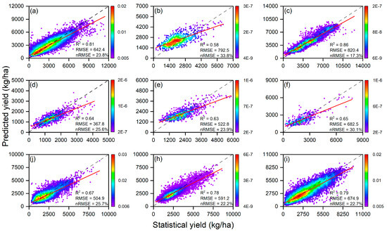
Figure 5.
Comparisons between the predicted yields of GlobalWheatYield4km and observed yields. (a) South and East Asia, (b) Central Asia, (c) Europe, (d) spring wheat in the Russian Federation and Kazakhstan, (e) winter wheat in the Russian Federation, (f) Australia, (g) South America, (h) spring wheat in North America, (i) winter wheat in North America. The color bar indicates the point density.
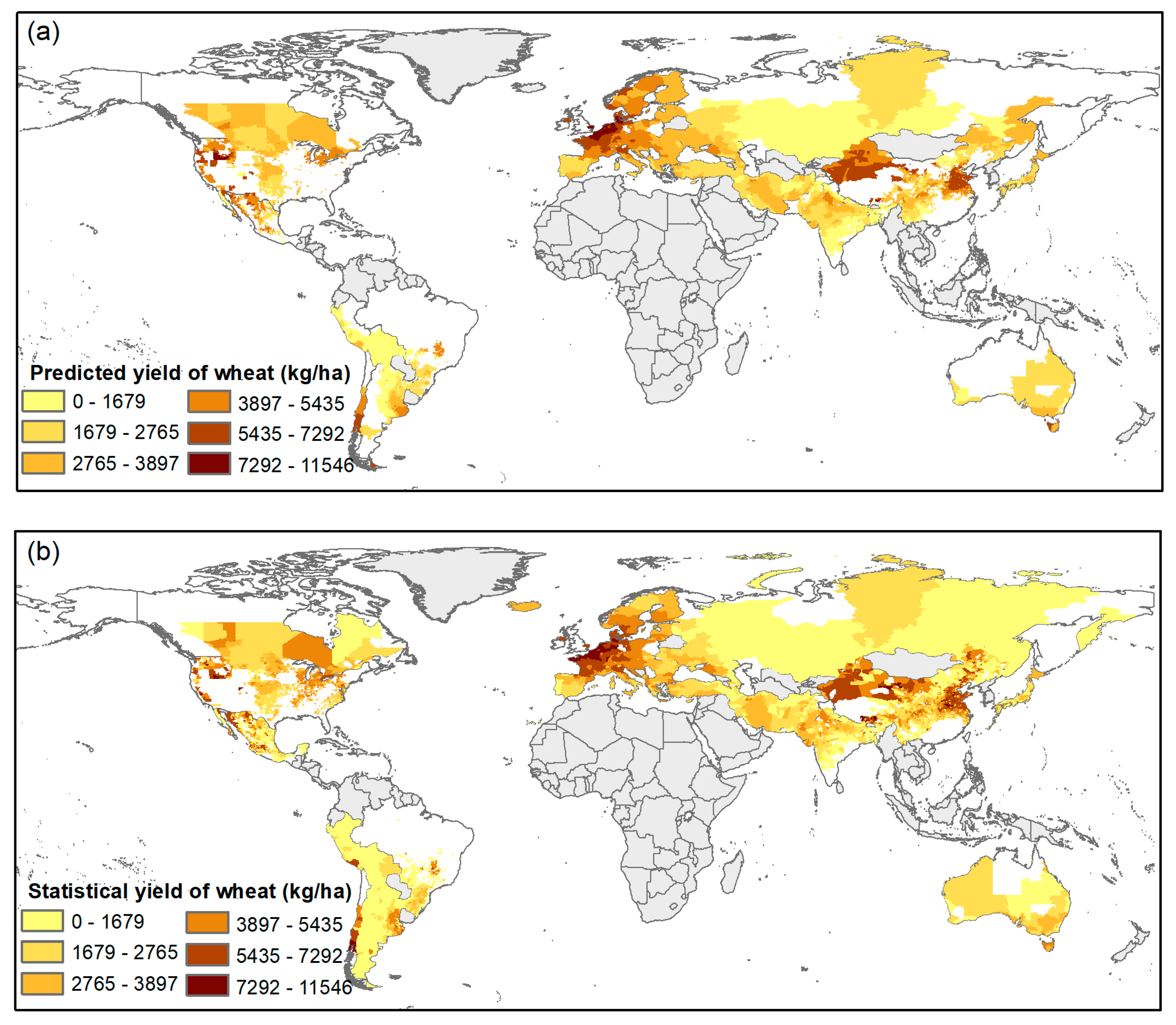
The spatial distributions of GlobalWheatYield4km were consistent with the observed yields in 2010 (Figure 6), with a large variability from 130 to 11,546 kg/ha. We further summarized the gridded yield by country. The average yields were the highest in Europe (e.g., Belgium: 8457 kg/ha; Netherlands: 8011 kg/ha), followed by Chile (5201 kg/ha) and China (4658 kg/ha). By contrast, Kazakhstan, Bangladesh, and Bolivia were indicated to have the lowest average yield (<1000 kg/ha). However, the spatial comparisons between predictions and statistical records indicated many blank values located in the prediction map, especially for two provinces (Newfoundland and Labrador) in Canada and most areas in Northern and Eastern Russia. We uncovered the missing data caused by their relatively sparce planting areas (Figure 6a) since our baseline map was derived by the criterion above 50% identification rate (at least 4 years) when identifying annual area dynamics during the period of 2006~2014.
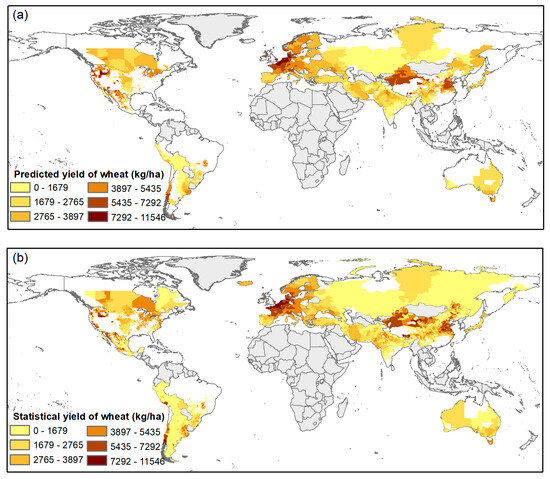
Figure 6.
Spatial distribution of the predicted yield aggregated over administrative unit level (a) and the observed yields (b) in 2010.
Besides the spatial distribution assessment above, we further assessed annual variation accuracy. The correlation coefficients between the time series of predicted and the observed yields for each subnational-level unit were summarized separately by main wheat planting regions in the world (Figure S3). We simultaneously found good temporal consistencies between the time series of GlobalWheatYield4km and observed yield. The average correlation coefficients (r values) ranged from 0.4 to 0.8, implying a strong temporal learning ability of our GWPMS method. More interestingly, GlobalWheatYield4km clearly indicated the impacts on yield from extreme events (Figure S5). For example, a drought that occurred in 2006 hit wheat production in Australia, and the predicted yields distinctly showed yield reductions in all regions across Australia, suggesting our GlobalWheatYield4km captures the spatiotemporal variability of wheat yields well at the subnational scale.
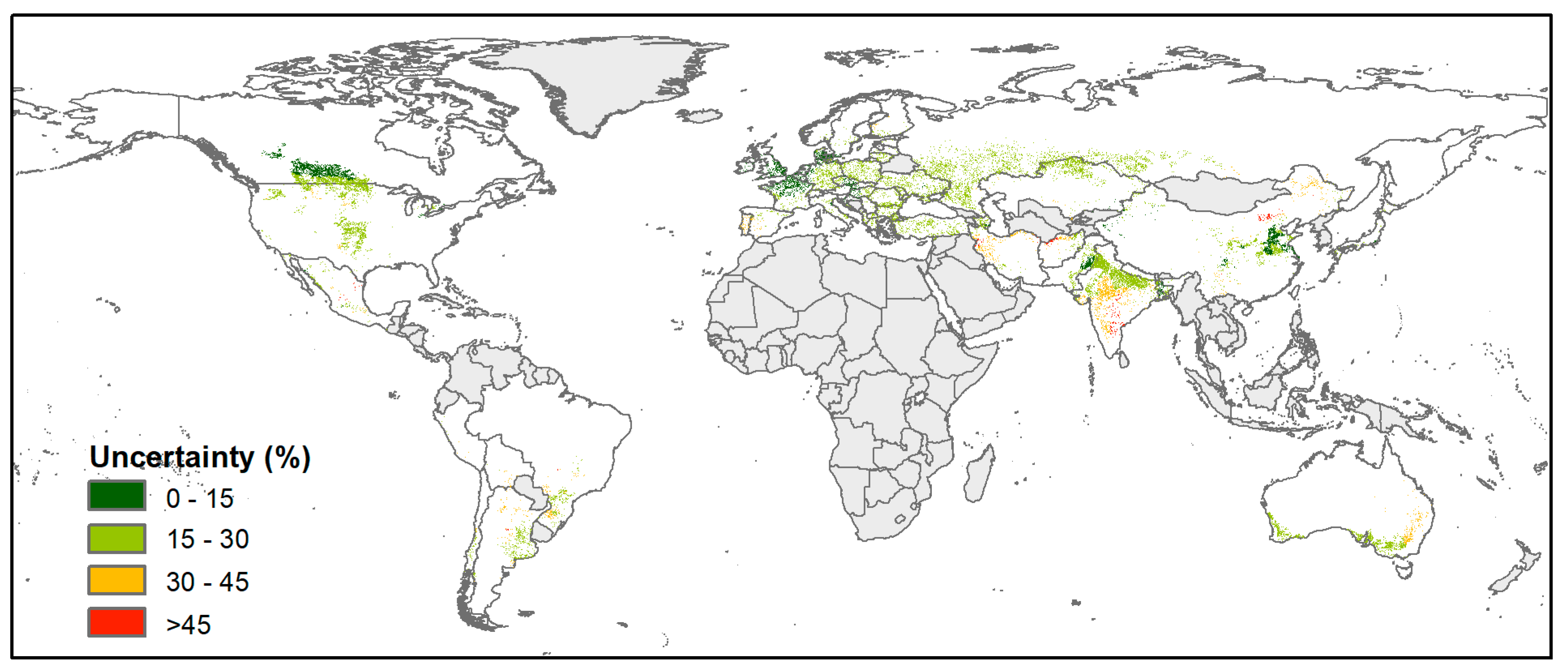
The nRMSE values in most areas (88.9% of grids) were below 30%, suggesting a higher accuracy. However, 2.9% of grids were indicated to have a higher nRMSE > 40%. Moreover, the regions with higher uncertainty are mainly located in Southern India, Western Afghanistan and Iran, Southern South America, Northeastern China, and Central Mexico, possibly due to the sparse distributions of wheat or short period of census data available there (Figure 7). Similarly, the lower errors, indicated by the nRMSE averages ranging from 13.7% to 37.9%, further evidence a strong temporal learning ability of our GWPMS method (Figure S5).
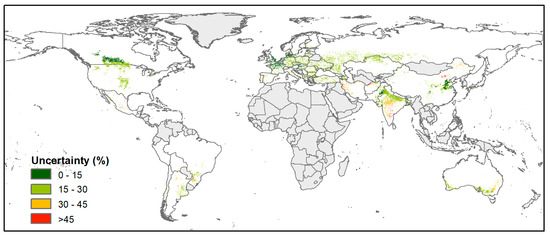
Figure 7.
Spatial distribution of uncertainty (i.e., nRMSE, %) in GlobalWheatYield4km.
3.3. Comparing GlobalWheatYield4km with SPAM
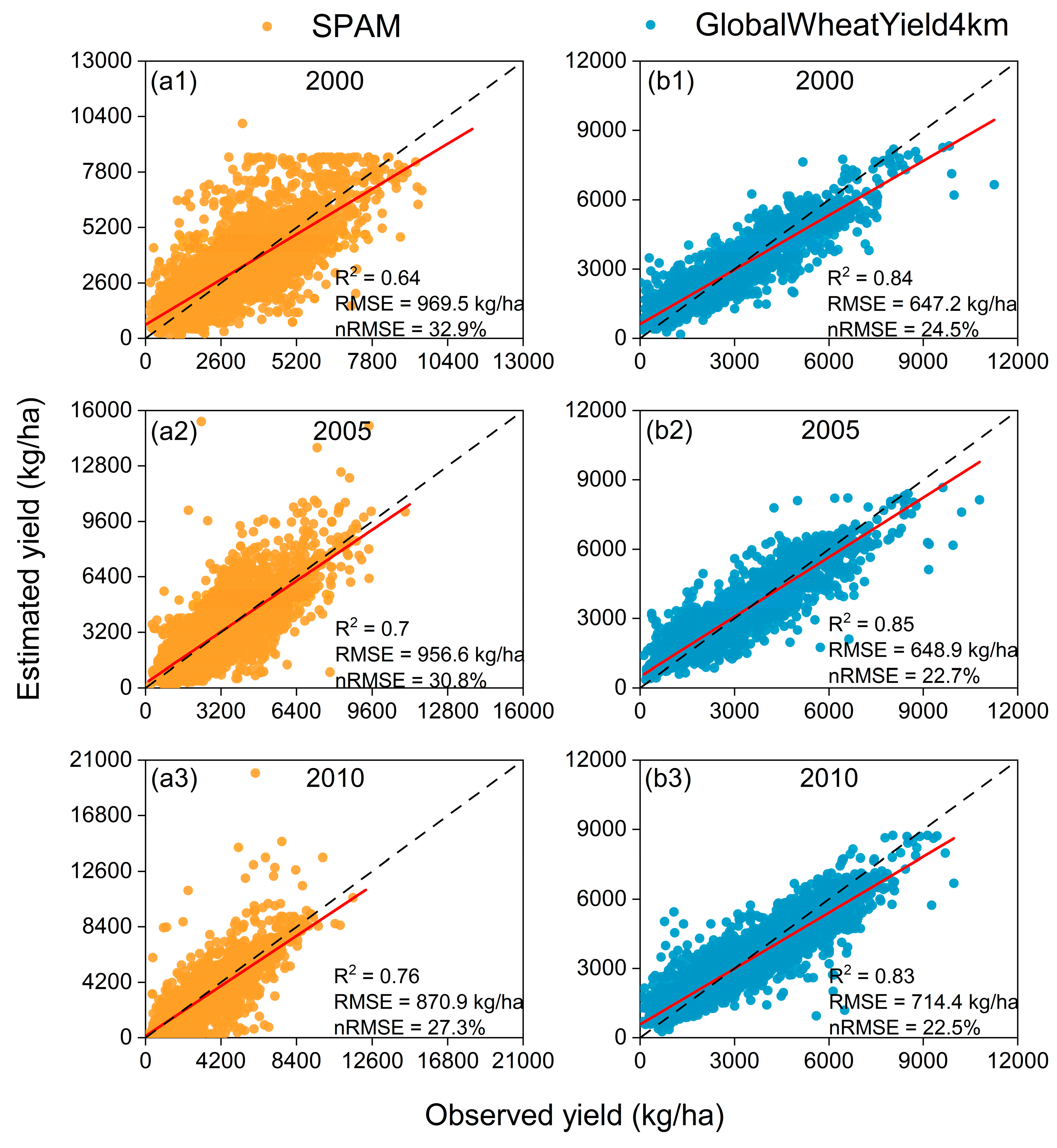
We aggregated gridded-yield estimates of GlobalWheatYield4km in 2000, 2005, and 2010 and the average of SPAM for three adjacent years to administrative units, and then compared them with census yields, respectively. Overall, the yield estimates of GlobalWheatYield4km showed higher consistencies with census yields as they were closer to the 1:1 line than SPAM, with an average R2 (RMSE) of 0.84 (670.2 kg/ha) and 0.7 (932.3 kg/ha), respectively (Figure 8). In addition, GlobalWheatYield4km exhibited higher and more robust accuracies than SPAM in all three years and regions (Figure S6 and Table S5). The R2 (RMSE) of GlobalWheatYield4km was improved (reduced) by an average of 42.2% (22.6%) as compared with SPAM, especially in Argentina, Australia, Iran, Pakistan, and the United States (improvements over 23% for R2 and RMSE). We ascribed such improvement to the consequent high-quality input data at more consistent and finer resolution. In contrast, the methodology and input data of SPAM were improved stepwise.
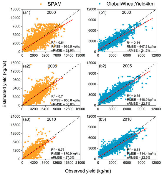
Figure 8.
Subnational-level comparisons between observed yields and estimated yields of SPAM (a1–a3) or GlobalWheatYield4km (b1–b3) for 2000 (a1,b1), 2005 (a2,b2), and 2010 (a3,b3).
4. Discussion
4.1. Advantages of GlobalWheatYield4km
GlobalWheatYield4km outperforms other global crop yield products (e.g., SPAM, GAEZ) with the following advantages: (a) the highest spatial resolution (4 km) among all yield datasets presently available; (b) higher accuracy as compared with SPAM; (c) clear subdivision of spring and winter wheat; and (d) clear characterization of the spatiotemporal dynamics of global wheat yields over 40 years. We compared two typical ML and DL models that are commonly used for yield prediction, determined the optimal model, and transferred them to generate gridded-yield estimates, which could improve the accuracy of our dataset. We found that LSTM consistently outperformed the RF model regardless of year and region, which was also confirmed by many previous studies [30,33,44,64]. The LSTM model, characterized by its recurrent neural network structure, has been widely proved to capture successfully cumulative and complex nonlinear relationships between crop yields and climatic factors [31,32,65,66].
Due to census data being unavailable, especially for the long term, it was very hard for us to collect finer-scale census data in some countries such as Kazakhstan and Afghanistan as well as Africa and Central Asia. Consequently, even compiling the detailed census data from the largest subnational units (~11,000), some data gaps are still left in some areas, similarly to the inconsistency among temporal periods and spatial distributions. Interestingly, the spatiotemporal transferable method we developed makes up for the above limitations by accurately estimating yields to some degree. Accordingly, we transferred the optimal model spatially and temporally to other areas and years with unavailable census data (Table S3) and provided the global wheat yield data with the highest resolution of 4 km and covering 40 years.
4.2. Uncertainties
Despite the higher accuracy of GlobalWheatYield4km, there were still some limitations. First, the largest constraint was the uncertainties of remote sensing data. For example, cloud and snow contaminations could cause noise in GLASS LAI products and consequently dampen the wheat detection signal [50]. The other uncertainty was from GFSAD1KCM, with a coarser resolution than GFSAD30 m FSAD products in accurately capturing the spatial distributions of cropland with respect to medium and small agriculture field sizes in some regions such as South Asia [67]. Algorithms do impact prediction accuracy, as evidenced by the comparison between the RF and LSTM models (Figure 4). With the rapid development in algorithms, many state-of-the-art deep learning techniques have been proposed. Among these, the attention model is one such hotspot proven to be more efficient especially for inference or prediction than LSTM [68,69]. Nevertheless, we should note that the accuracy of predictions is depended strongly on the quantity and quality of observed samples (Figure 4 and Figure 7).
Moreover, the spatial resolution of 1 km could result in mixed pixel issues, potentially lowering our dataset accuracy, especially in areas where wheat was sparsely cultivated (e.g., South America). Nevertheless, two approaches can offset these impacts to some degree. First, the cultivation pattern is complicated in the main wheat-planting areas (e.g., the North China Plain in China, Saskatchewan in Canada, North Dakota in the United States, and Northern India). These areas are cultivated with complicated patterns in small fields generally behaving like “large fields” and consequently weakening the impacts of mixed pixel issues [52]. In addition, to avoid the misclassification of pixels, we integrated the annual 1 km map during 2006–2014 to generate a baseline map with the grids with wheat-planting areas for at least 4 years, which consequently purified pixels to some degree. Therefore, it should be noted that potential users should mask our products with explicitly annual wheat planting maps to obtain accurate yield data, especially for the annual growing areas changing significantly over time. We will try to map the spatial distribution of wheat using remote sensing images with finer spatial resolutions in the future and further improve yield estimates [70,71].
5. Conclusions
Here, we proposed a spatiotemporal transferable method to estimate global wheat yield at a 4 km resolution over four decades using data-driven models (available at https://doi.org/10.6084/m9.figshare.10025006). We firstly identified the spatial distribution of wheat harvesting areas using a spectra–phenology integration method then developed ML and DL models and transferred the optimal models to estimate yield at the grid scale. The distribution map showed a high accuracy, with an R2 of 0.8. The optimal models (LSTM, R2 = 0.72, nRMSE = 13.1%) were transferred into global wheat planting areas across 40 years and obtained the first global yield estimate product with a higher resolution. We comprehensively assessed the accuracy at both spatial and temporal scales. Our GlobalWheatYield4km indicates high spatial consistency with observed yields, with an R2 (RMSE) of 0.82 (619.8 kg/ha). Good temporal consistency is further evidenced by r values (0.4~0.8) and nRMSE (13.7~37.9%) across all subnational regions covering 40 years. As compared with another public product, GlobalWheatYield4km showed 45% higher accuracy (R2~0.71) than SPAM (R2~0.49). The resultant dataset can benefit many studies, including agricultural system modeling and climate change impact assessments over larger regions.
Supplementary Materials
The following supporting information can be downloaded at https://www.mdpi.com/article/10.3390/rs16132342/s1.
Author Contributions
Conceptualization, Z.Z.; Data curation, J.H.; Formal analysis, Y.L.; Methodology, Y.L.; Validation, J.X.; Visualization, J.H.; Writing—original draft, Y.L.; Writing—review & editing, F.T. All authors have read and agreed to the published version of the manuscript.
Funding
This study was funded by National Natural Science Foundation of China (42061144003, 41977405).
Data Availability Statement
The data presented in this study are openly available at https://doi.org/10.6084/m9.figshare.10025006.
Conflicts of Interest
The authors declare no conflict of interest.
References
- FAO; IFAD; UNICEF; WFP; WHO. Transforming Food Systems for Affordable Healthy Diets. In The State of Food Security and Nutrition in the World 2020; FAO: Rome, Italy, 2020. [Google Scholar] [CrossRef]
- United Nations. Sustainable Development Goal 2. Sustainable Development Knowledge Platform. 2017. Available online: https://sustainabledevelopment.un.org/sdg2 (accessed on 19 June 2024).
- International Food Policy Research Institute. 2022 Global Food Policy Report: Climate Change and Food Systems; International Food Policy Research Institute: Washington, DC, USA, 2022. [Google Scholar] [CrossRef]
- FAO; IFAD; UNICEF; WFP; WHO. Transforming food systems for food security, improved nutrition and affordable healthy diets for all. In The State of Food Security and Nutrition in the World 2020; FAO: Rome, Italy, 2021. [Google Scholar] [CrossRef]
- Sulser, T.; Wiebe, K.D.; Dunston, S.; Cenacchi, N.; Nin-Pratt, A.; Mason-D’Croz, D.; Robertson, R.D.; Willenbockel, D.; Rosegrant, M.W. Climate change and hunger: Estimating costs of adaptation in the agrifood system. In Food Policy Report June 2021; International Food Policy Research Institute (IFPRI): Washington, DC, USA, 2021. [Google Scholar] [CrossRef]
- van Dijk, M.; Morley, T.; Rau, M.L.; Saghai, Y. A meta-analysis of projected global food demand and population at risk of hunger for the period 2010–2050. Nat. Food 2021, 2, 494–501. [Google Scholar] [CrossRef]
- Folberth, C.; Khabarov, N.; Balkovic, J.; Skalsky, R.; Visconti, P.; Ciais, P.; Janssens, I.A.; Penuelas, J.; Obersteiner, M. The global cropland-sparing potential of high-yield farming. Nat. Sustain. 2020, 3, 281–289. [Google Scholar] [CrossRef]
- Lobell, D.B.; Cassman, K.G.; Field, C.B. Crop Yield Gaps: Their Importance, Magnitudes, and Causes. Annu. Rev. Environ. Resour. 2009, 34, 179–204. [Google Scholar] [CrossRef]
- Ray, D.K.; Gerber, J.S.; MacDonald, G.K.; West, P.C. Climate variation explains a third of global crop yield variability. Nat. Commun. 2015, 6, 5989. [Google Scholar] [CrossRef]
- Rötter, R.P.; Hoffmann, M.P.; Koch, M.; Müller, C. Progress in modelling agricultural impacts of and adaptations to climate change. Curr. Opin. Plant Biol. 2018, 45, 255–261. [Google Scholar] [CrossRef] [PubMed]
- Balaghi, R.; Tychon, B.; Eerens, H.; Jlibene, M. Empirical regression models using NDVI, rainfall and temperature data for the early prediction of wheat grain yields in Morocco. Int. J. Appl. Earth Obs. 2008, 10, 438–452. [Google Scholar] [CrossRef]
- Bussay, A.; van der Velde, M.; Fumagalli, D.; Seguini, L. Improving operational maize yield forecasting in Hungary. Agric. Syst. 2015, 141, 94–106. [Google Scholar] [CrossRef]
- Feng, L.W.; Wang, Y.M.; Zhang, Z.; Du, Q.Y. Geographically and temporally weighted neural network for winter wheat yield prediction. Remote Sens. Environ. 2021, 262, 112514. [Google Scholar] [CrossRef]
- Franch, B.; Vermote, E.F.; Becker-Reshef, I.; Claverie, M.; Huang, J.; Zhang, J.; Justice, C.; Sobrino, J.A. Improving the timeliness of winter wheat production forecast in the United States of America, Ukraine and China using MODIS data and NCAR Growing Degree Day information. Remote Sens. Environ. 2015, 161, 131–148. [Google Scholar] [CrossRef]
- Jin, Z.N.; Azzari, G.; Lobell, D.B. Improving the accuracy of satellite-based high-resolution yield estimation: A test of multiple scalable approaches. Agric. For. Meteorol. 2017, 247, 207–220. [Google Scholar] [CrossRef]
- Zhao, Y.; Potgieter, A.B.; Zhang, M.; Wu, B.F.; Hammer, G.L. Predicting Wheat Yield at the Field Scale by Combining High-Resolution Sentinel-2 Satellite Imagery and Crop Modelling. Remote Sens. 2020, 12, 1024. [Google Scholar] [CrossRef]
- Chen, Y.; Tao, F.L. Potential of remote sensing data-crop model assimilation and seasonal weather forecasts for early-season crop yield forecasting over a large area. Field Crop. Res. 2022, 276, 108398. [Google Scholar] [CrossRef]
- Huang, J.X.; Gomez-Dans, J.L.; Huang, H.; Ma, H.Y.; Wu, Q.L.; Lewis, P.E.; Liang, S.L.; Chen, Z.X.; Xue, J.H.; Wu, Y.T.; et al. Assimilation of remote sensing into crop growth models: Current status and perspectives. Agric. For. Meteorol. 2019, 276, 107609. [Google Scholar] [CrossRef]
- Ines, A.V.M.; Das, N.N.; Hansen, J.W.; Njoku, E.G. Assimilation of remotely sensed soil moisture and vegetation with a crop simulation model for maize yield prediction. Remote Sens. Environ. 2013, 138, 149–164. [Google Scholar] [CrossRef]
- Luo, Y.C.; Zhang, Z.; Zhang, L.L.; Cao, J. Spatiotemporal patterns of winter wheat phenology and its climatic drivers based on an improved pDSSAT model. Sci. China Earth Sci. 2021, 64, 2144–2160. [Google Scholar] [CrossRef]
- Zhuo, W.; Fang, S.B.; Gao, X.R.; Wang, L.; Wu, D.; Fu, S.L.; Wu, Q.L.; Huang, J.X. Crop yield prediction using MODIS LAI, TIGGE weather forecasts and WOFOST model: A case study for winter wheat in Hebei, China during 2009–2013. Int. J. Appl. Earth Obs. 2022, 106, 102668. [Google Scholar] [CrossRef]
- Burke, M.; Lobell, D.B. Satellite-based assessment of yield variation and its determinants in smallholder African systems. Proc. Natl. Acad. Sci. USA 2017, 114, 2189–2194. [Google Scholar] [CrossRef] [PubMed]
- Kern, A.; Barcza, Z.; Marjanovic, H.; Arendas, T.; Fodor, N.; Bonis, P.; Bognar, P.; Lichtenberger, J. Statistical modelling of crop yield in Central Europe using climate data and remote sensing vegetation indices. Agric. For. Meteorol. 2018, 260, 300–320. [Google Scholar] [CrossRef]
- Lobell, D.B.; Burke, M.B. On the use of statistical models to predict crop yield responses to climate change. Agric. For. Meteorol. 2010, 150, 1443–1452. [Google Scholar] [CrossRef]
- Cai, Y.P.; Guan, K.Y.; Lobell, D.; Potgieter, A.B.; Wang, S.W.; Peng, J.; Xu, T.F.; Asseng, S.; Zhang, Y.G.; You, L.Z.; et al. Integrating satellite and climate data to predict wheat yield in Australia using machine learning approaches. Agric. For. Meteorol. 2019, 274, 144–159. [Google Scholar] [CrossRef]
- Cao, J.; Zhang, Z.; Tao, F.L.; Zhang, L.L.; Luo, Y.C.; Zhang, J.; Han, J.C.; Xie, J. Integrating Multi-Source Data for Rice Yield Prediction across China using Machine Learning and Deep Learning Approaches. Agric. For. Meteorol. 2021, 297, 108275. [Google Scholar] [CrossRef]
- Li, L.C.; Wang, B.; Feng, P.Y.; Wang, H.H.; He, Q.S.; Wang, Y.K.; Liu, D.L.; Li, Y.; He, J.Q.; Feng, H.; et al. Crop yield forecasting and associated optimum lead time analysis based on multi-source environmental data across China. Agric. For. Meteorol. 2021, 308, 108558. [Google Scholar] [CrossRef]
- Jin, S.C.; Su, Y.; Gao, S.; Hu, T.Y.; Liu, J.; Guo, Q.H. The Transferability of Random Forest in Canopy Height Estimation from Multi-Source Remote Sensing Data. Remote Sens. 2018, 10, 1183. [Google Scholar] [CrossRef]
- Kang, Y.H.; Ozdogan, M.; Zhu, X.J.; Ye, Z.W.; Hain, C.; Anderson, M. Comparative assessment of environmental variables and machine learning algorithms for maize yield prediction in the US Midwest. Environ. Res. Lett. 2020, 15, 064005. [Google Scholar] [CrossRef]
- Jeong, S.; Ko, J.; Yeom, J.M. Predicting rice yield at pixel scale through synthetic use of crop and deep learning models with satellite data in South and North Korea. Sci. Total Environ. 2022, 802, 149726. [Google Scholar] [CrossRef]
- Zhang, L.L.; Zhang, Z.; Luo, Y.C.; Cao, J.; Xie, R.Z.; Li, S.K. Integrating satellite-derived climatic and vegetation indices to predict smallholder maize yield using deep learning. Agric. For. Meteorol. 2021, 311, 108666. [Google Scholar] [CrossRef]
- Jiang, H.; Hu, H.; Zhong, R.H.; Xu, J.F.; Xu, J.L.; Huang, J.F.; Wang, S.W.; Ying, Y.B.; Lin, T. A deep learning approach to conflating heterogeneous geospatial data for corn yield estimation: A case study of the US Corn Belt at the county level. Glob. Chang. Biol. 2020, 26, 1754–1766. [Google Scholar] [CrossRef]
- Tian, H.R.; Wang, P.X.; Tansey, K.; Zhang, J.Q.; Zhang, S.Y.; Li, H.M. An LSTM neural network for improving wheat yield estimates by integrating remote sensing data and meteorological data in the Guanzhong Plain, PR China. Agric. For. Meteorol. 2021, 310, 108629. [Google Scholar] [CrossRef]
- Lesk, C.; Rowhani, P.; Ramankutty, N. Influence of extreme weather disasters on global crop production. Nature 2016, 529, 84–87. [Google Scholar] [CrossRef]
- Lobell, D.B.; Hammer, G.L.; McLean, G.; Messina, C.; Roberts, M.J.; Schlenker, W. The critical role of extreme heat for maize production in the United States. Nat. Clim. Chang. 2013, 3, 497–501. [Google Scholar] [CrossRef]
- Weiss, M.; Jacob, F.; Duveiller, G. Remote sensing for agricultural applications: A meta-review. Remote Sens. Environ. 2020, 236, 111402. [Google Scholar] [CrossRef]
- Monfreda, C.; Ramankutty, N.; Foley, J.A. Farming the planet: 2. Geographic distribution of crop areas, yields, physiological types, and net primary production in the year 2000. Glob. Biogeochem. Cycles 2008, 22, GB1022. [Google Scholar] [CrossRef]
- Fischer, G.; Nachtergaele, F.O.; Prieler, S.; Teixeira, E.; Tóth, G.; Velthuizen, H.V.; Verelst, L.; Wiberg, D. Global Agro-Ecological Zones (GAEZ v3.0); IIASA: Laxenburg, Austria; FAO: Rome, Italy, 2012. [Google Scholar]
- You, L.Z.; Wood, S.; Wood-Sichra, U.; Wu, W.B. Generating global crop distribution maps: From census to grid. Agric. Syst. 2014, 127, 53–60. [Google Scholar] [CrossRef]
- Grogan, D.; Frolking, S.; Wisser, D.; Prusevich, A.; Glidden, S. Global gridded crop harvested area, production, yield, and monthly physical area data circa 2015. Sci. Data 2022, 9, 15. [Google Scholar] [CrossRef]
- Tao, F.; Yokozawa, M.; Zhang, Z. Modelling the impacts of weather and climate variability on crop productivity over a large area: A new process-based model development, optimization, and uncertainties analysis. Agric. For. Meteorol. 2009, 149, 831–850. [Google Scholar] [CrossRef]
- Tao, F.L.; Yokozawa, M.; Xu, Y.L.; Hayashi, Y.; Zhang, Z. Climate changes and trends in phenology and yields of field crops in China, 1981–2000. Agric. For. Meteorol. 2006, 138, 82–92. [Google Scholar] [CrossRef]
- Iizumi, T.; Sakai, T. The global dataset of historical yields for major crops 1981–2016. Sci. Data 2020, 7, 97. [Google Scholar] [CrossRef]
- Luo, Y.C.; Zhang, Z.; Cao, J.; Zhang, L.L.; Zhang, J.; Han, J.C.; Zhuang, H.M.; Cheng, F.; Tao, F.L. Accurately mapping global wheat production system using deep learning algorithms. Int. J. Appl. Earth Obs. 2022, 110, 102823. [Google Scholar] [CrossRef]
- FAOSTAT. Food and Agriculture Organization of the United Nations Statistics Division. 2020. Available online: http://www.fao.org/faostat/en/#data (accessed on 19 June 2024).
- Ren, S.L.; Qin, Q.M.; Ren, H.Z. Contrasting wheat phenological responses to climate change in global scale. Sci. Total Environ. 2019, 665, 620–631. [Google Scholar] [CrossRef]
- USDA. Major world crop areas and climatic profiles. In Agricultural Handbook; USDA: Washington, DC, USA, 1994; Volume 664, p. 279. [Google Scholar]
- Vermote, E.; Justice, C.; Csiszar, I.; Eidenshink, J.; Myneni, R.; Baret, F.; Masuoka, E.; Wolfe, R.; Claverie, M. NOAA CDR Program: NOAA Climate Data Record (CDR) of Normalized Difference Vegetation Index (NDVI), Version 5; NOAA National Climatic Data Center: Asheville, NC, USA, 2014. [Google Scholar] [CrossRef]
- Xiao, Z.Q.; Liang, S.L.; Wang, J.D.; Xiang, Y.; Zhao, X.; Song, J.L. Long-Time-Series Global Land Surface Satellite Leaf Area Index Product Derived from MODIS and AVHRR Surface Reflectance. IEEE Trans. Geosci. Remote Sens. 2016, 54, 5301–5318. [Google Scholar] [CrossRef]
- Xiao, Z.Q.; Liang, S.L.; Wang, J.D.; Chen, P.; Yin, X.J.; Zhang, L.Q.; Song, J.L. Use of General Regression Neural Networks for Generating the GLASS Leaf Area Index Product from Time-Series MODIS Surface Reflectance. IEEE Trans. Geosci. Remote Sens. 2014, 52, 209–223. [Google Scholar] [CrossRef]
- Teluguntla, P.; Thenkabail, P.; Xiong, J.; Gumma, M.; Giri, C.; Milesi, C.; Ozdogan, M.; Congalton, R.; Tilton, J.; Sankey, T.; et al. NASA Making Earth System Data Records for Use in Research Environments (MEaSUREs) Global Food Security Support Analysis Data (GFSAD) Crop Mask 2010 Global 1 km V001 [Data set]. NASA EOSDIS Land Processes DAAC; U.S. Geological Survey: Reston, VA, USA, 2016. [Google Scholar] [CrossRef]
- Luo, Y.C.; Zhang, Z.; Li, Z.Y.; Chen, Y.; Zhang, L.L.; Cao, J.; Tao, F.L. Identifying the spatiotemporal changes of annual harvesting areas for three staple crops in China by integrating multi-data sources. Environ. Res. Lett. 2020, 15, 074003. [Google Scholar] [CrossRef]
- Abatzoglou, J.T.; Dobrowski, S.Z.; Parks, S.A.; Hegewisch, K.C. TerraClimate, a high-resolution global dataset of monthly climate and climatic water balance from 1958–2015. Sci. Data 2018, 5, 170191. [Google Scholar] [CrossRef]
- Nachtergaele, F.O.; van Velthuizen, H.; Verelst, L.; Wiberg, D.; Batjes, N.H.; Dijkshoorn, J.A.; van Engelen, V.W.P.; Fischer, G.; Jones, A.; Montanarella, L.; et al. Harmonized World Soil Database (Version 1.2). Food and Agriculture Organization of the UN, International Institute for Applied Systems Analysis, ISRIC—World Soil Information, Institute of Soil Science—Chinese Academy of Sciences, Joint Research Centre of the EC. 2012. Available online: http://www.iiasa.ac.at/Research/LUC/External-World-soil-database/HWSD_Documentation.pdf (accessed on 4 August 2022).
- Dong, J.W.; Xiao, X.M.; Kou, W.L.; Qin, Y.W.; Zhang, G.L.; Li, L.; Jin, C.; Zhou, Y.T.; Wang, J.; Biradar, C.; et al. Tracking the dynamics of paddy rice planting area in 1986–2010 through time series Landsat images and spectra-phenology integration algorithms. Remote Sens. Environ. 2015, 160, 99–113. [Google Scholar] [CrossRef]
- Song, X.P.; Potapov, P.V.; Krylov, A.; King, L.; Di Bella, C.M.; Hudson, A.; Khan, A.; Adusei, B.; Stehman, S.V.; Hansen, M.C. National-scale soybean mapping and area estimation in the United States using medium resolution satellite imagery and field survey. Remote Sens. Environ. 2017, 190, 383–395. [Google Scholar] [CrossRef]
- Waldhof, G.; Lussem, U.; Bareth, G. Multi-Data Approach for remote sensing-based regional crop rotation mapping: A case study for the Rur catchment, Germany. Int. J. Appl. Earth Obs. 2017, 61, 55–69. [Google Scholar] [CrossRef]
- Geng, L.Y.; Ma, M.G.; Wang, X.F.; Yu, W.P.; Jia, S.Z.; Wang, H.B. Comparison of Eight Techniques for Reconstructing Multi-Satellite Sensor Time-Series NDVI Data Sets in the Heihe River Basin, China. Remote Sens. 2014, 6, 2024–2049. [Google Scholar] [CrossRef]
- Savitzky, A.; Golay, M.J.E. Smoothing and Differentiation of Data by Simplified Least Squares Procedures. Anal. Chem. 1964, 36, 1627–1639. [Google Scholar] [CrossRef]
- Wang, C.Z.; Zhang, Z.; Chen, Y.; Tao, F.L.; Zhang, J.; Zhang, W. Comparing different smoothing methods to detect double-cropping rice phenology based on LAI products—A case study in the Hunan province of China. Int. J. Remote Sens. 2018, 39, 6405–6428. [Google Scholar] [CrossRef]
- Breiman, L. Random forests. Mach. Learn. 2001, 45, 5–32. [Google Scholar] [CrossRef]
- Hochreiter, S.; Schmidhuber, J. Long short-term memory. Neural Comput. 1997, 9, 1735–1780. [Google Scholar] [CrossRef] [PubMed]
- You, N.S.; Dong, J.W. Examining earliest identifiable timing of crops using all available Sentinel 1/2 imagery and Google Earth Engine. ISPRS J. Photogramm. Remote Sens. 2020, 161, 109–123. [Google Scholar] [CrossRef]
- Schwalbert, R.A.; Amado, T.; Corassa, G.; Pott, L.P.; Prasad, P.V.V.; Ciampitti, I.A. Satellite-based soybean yield forecast: Integrating machine learning and weather data for improving crop yield prediction in southern Brazil. Agric. For. Meteorol. 2020, 284, 107886. [Google Scholar] [CrossRef]
- Joshi, A.; Pradhan, B.; Gite, S.; Chakraborty, S. Remote-sensing data and deep-Learning techniques in crop mapping and yield prediction: A systematic review. Remote Sens. 2023, 15, 2014. [Google Scholar] [CrossRef]
- Fei, S.; Hassan, M.A.; Xiao, Y.; Su, X.; Chen, Z.; Cheng, Q.; Chen, R.; Ma, Y. UAV-based multi-sensor data fusion and machine learning algorithm for yield prediction. Precis. Agric. 2023, 24, 187–212. [Google Scholar] [CrossRef]
- Yadav, K.; Congalton, R.G. Accuracy Assessment of Global Food Security-Support Analysis Data (GFSAD) Cropland Extent Maps Produced at Three Different Spatial Resolutions. Remote Sens. 2018, 10, 1800. [Google Scholar] [CrossRef]
- Niu, Z.; Zhong, G.; Yu, H. A review on the attention mechanism of deep learning. Neurocomputing 2021, 452, 48–62. [Google Scholar] [CrossRef]
- Sun, Z.; Li, Q.; Jin, S.; Song, Y.; Xu, S.; Wang, X.; Cai, J.; Zhou, Q.; Ge, Y.; Zhang, R.; et al. Simultaneous prediction of wheat yield and grain protein content using multitask deep learning from time-series proximal sensing. Plant Phenom. 2022, 2022, 9757948. [Google Scholar] [CrossRef] [PubMed]
- Wang, S.; Di Tommaso, S.; Deines, J.M.; Lobell, D.B. Mapping twenty years of corn and soybean across the US Midwest using the Landsat archive. Sci. Data 2020, 7, 307. [Google Scholar] [CrossRef]
- Niu, Q.D.; Li, X.C.; Huang, J.X.; Huang, H.; Huang, X.D.; Su, W.; Yuan, W.P. A 30 m annual maize phenology dataset from 1985 to 2020 in China. Earth Syst. Sci. Data 2022, 14, 2851–2864. [Google Scholar] [CrossRef]
Disclaimer/Publisher’s Note: The statements, opinions and data contained in all publications are solely those of the individual author(s) and contributor(s) and not of MDPI and/or the editor(s). MDPI and/or the editor(s) disclaim responsibility for any injury to people or property resulting from any ideas, methods, instructions or products referred to in the content. |
© 2024 by the authors. Licensee MDPI, Basel, Switzerland. This article is an open access article distributed under the terms and conditions of the Creative Commons Attribution (CC BY) license (https://creativecommons.org/licenses/by/4.0/).

