Abstract
Image super-resolution (SR) technology can improve the resolution of images and provide clearer and more reliable remote sensing images of high quality to better serve the subsequent applications. However, when reconstructing high-frequency feature areas of remote sensing images, existing SR reconstruction methods are prone to artifacts that affect visual effects and make it difficult to generate real texture details. In order to address this issue, a texture-detail-enhanced dense generative adversarial network (TDEGAN) for remote sensing image SR is presented. The generator uses multi-level dense connections, residual connections, and Shuffle attention (SA) to improve the feature extraction ability. A PatchGAN-style discrimination network is designed to effectively perform local discrimination and helps the network generate rich, detailed features. To reduce the impact of artifacts, we introduce an artifact loss function, which is combined with the exponential moving average (EMA) technique to distinguish the artifacts generated from the actual texture details through local statistics, which can help the network reduce artifacts and generate more realistic texture details. Experiments show that TDEGAN can better restore the texture details of remote sensing images and achieves certain advantages in terms of evaluation indicators and visualization.
1. Introduction
The increasing maturity of remote sensing technology enables researchers to obtain rich surface observation images and serve all walks of life in society. However, due to the limitations of the imaging hardware, technology, and observation environment of remote sensing images [1], obtaining high-resolution (HR) remote sensing images takes work. The quality of low-resolution (LR) remote sensing images is not sufficient for the application of remote sensing images in map updating [2], semantic segmentation [3], and target detection [4]. Therefore, remote sensing image SR reconstruction technology has become a vital processing technology for improving the clarity and reliability of remote sensing images at low cost. The local unmixing ability of SR reconstruction technology can make observations in remote sensing images more prominent, providing more reliable data for subsequent remote sensing image processing. For example, researchers can use SR reconstruction technology to more accurately extract buildings from and detect changes in target boundaries in remote sensing images [5]. SR technology was also used to achieve the precise labeling of hyperspectral images [6] and address fusion-related issues [7]. The realization of remote sensing image SR reconstruction technology from an algorithmic perspective has become an important research topic in image processing and computer vision [8].
Image SR reconstruction is a technique that uses LR images to reconstruct HR images with richer information. Interpolation-based methods, reconstruction-based methods, and learning-based methods are three types of image SR reconstruction methods. Interpolation-based methods mainly rely on mathematical interpolation techniques. By utilizing the numerical information of known points and their positional relationships in space, interpolation algorithms are used to infer the values of unknown points, achieving improved image resolution. Interpolation-based methods mainly include nearest-neighbor interpolation [9], bicubic interpolation [10], and bilinear interpolation [11], among others. Although these methods have the characteristics of simple computation and high efficiency, it is often challenging for them to capture the high-frequency detail information of images, resulting in unsatisfactory performance in handling complex textures and edges. Reconstruction-based methods are usually based on signal reconstruction theory. The process of downsampling HR images to LR images is used as prior information to construct an observation model. Regularization methods are used to construct prior constraints of HR images. It is transformed into a cost function optimization problem under a constraint condition to achieve image super-resolution reconstruction. Reconstruction-based methods mainly include the iterative back projection method [12], maximum posterior estimation method [13], and convex set projection method [14]. Although reconstruction-based methods have good reconstruction results, when the amplification coefficient is significant, the learning difficulty of this method increases sharply, and, due to limited prior information, some texture details are difficult to recover. Learning-based methods achieve SR reconstruction by learning the mapping relationship between HR images and LR images in feature space. Learning-based methods can be divided into three categories: neighborhood embedding methods [15], sparse representation methods [16], and deep learning methods [17]. In recent years, the mature application of artificial intelligence technology in many fields has also brought many new solutions to the challenges faced by image SR reconstruction technology. Some image SR methods developed by scientific researchers based on the deep learning framework and neural network ideas have achieved excellent reconstruction quality [18]. The image SR reconstruction method based on deep learning uses neural networks to map the LR feature space to the HR feature space which automatically learn this mapping function through large-scale training data to effectively convert LR images into HR images. Deep learning methods typically involve two main branches: SR reconstruction based on a convolutional neural networks (CNN) and SR reconstruction based on a generative adversarial network (GAN).
The CNN-based method uses CNN structures, such as convolution layers and pooling layers, to extract features from LR images and gradually map them to HR images [19]. In 2014, Dong et al. presented a simple SR reconstruction using a CNN (SRCNN) [20], becoming the first to introduce a CNN into the field of image SR. This network consisted of only three layers of CNNs, each with different convolution kernel sizes and filter numbers, enhancing the network’s feature extraction ability. In addition, nonlinear mapping functions were added after each convolution layer, further enhancing the network’s nonlinear expression ability. SRCNN can generate images with better visual perception than traditional image SR reconstruction methods. However, due to the generation network having fewer layers and the large convolution kernel, it is difficult for it to extract the deep features of the image, and the reconstructed image loses some details. In 2016, Chao et al. presented a fast SR reconstruction method based on a CNN (FSRCNN) [21]. FSRCNN adopts smaller convolution kernels to simplify the network structure, and uses small-sized filters to process images to reduce computational complexity. This method converts LR images to HR images through convolution and deconvolution layers [22]. FSRCNN achieved higher evaluation scores and better image reconstruction results. In the same year, Kim et al. increased the depth of the model, enabling the network to extract hierarchical feature information better, and presented a deeply recursive convolution network (DRCN) [23]. This method uses skip connection and recursive supervision to enhance training stability and improve the model’s reconstructed image performance. In 2017, Lim et al. presented the enhanced residual network (EDSR) [24] for SR reconstruction based on the CNN and residual network (ResNet) ideas [25], applying ResNet to the field of image SR reconstruction. In EDSR, the researchers chose to remove the batch normalization (BN) layer from ResNet, freeing up computational resources and allowing for more network layers to be added under the same resources, thereby improving the feature extraction ability of each layer of the network. The CNN-based methods have made significant progress in image SR reconstruction tasks, but they also have some shortcomings and challenges. In particular, the commonly used mean square error (MSE) loss function may lead to the model having the tendency to generate images with higher peak signal-to-noise ratio indicators [20] and lacking high-frequency features, making it difficult to generate more realistic texture details.
The GAN-based method introduces the generation network and the discrimination network, which can generate more realistic textures through adversarial training [26]. In 2017, Ledig et al. used GAN architecture for the first time to achieve image SR reconstruction and developed an image SR reconstruction method using a GAN (SRGAN) [27]. SRGAN uses deep residual networks and upsampling layers to convert LR images into HR images and uses perceptual loss [28] in adversarial training to effectively increase the texture details and clarity of the image. Perception loss is based on a pre-trained CNN (VGG networks) and compares the feature differences between generated and authentic images. This helps generate more realistic images and solves the problem where using the MSE loss function causes images to be too smooth. With the introduction of SRGAN, many image SR reconstruction models based on GANs have been presented. In 2018, Wang et al. presented an enhanced SRGAN (ESRGAN) [29]. A residual-in-residual dense block (RRDB) was designed to replace ResNet, which can help the network better learn residual information and generate more realistic and clear images. ESRGAN removes all BN layers, which can improve the evaluation metrics of SR, reduce computational complexity, and save memory. It uses a perceptual loss function before activation, which can solve the problem of sparse feature quantities. In 2020, Carraz et al. presented ESRGAN+ [30], which incorporates residual connections and noise in an RRDB to enhance the generation network’s ability to extract features. In 2021, Wang et al. presented Real-ESRGAN [31], replacing the VGG-style discrimination network in ESRGAN with a U-Net discrimination network. Image SR reconstruction is achieved by simulating various degradations during the conversion from HR to LR, which has good reconstruction results in anime images and videos. However, it should be pointed out that adversarial training still has the problem of training instability in this field, which can generate unpleasant artifacts during the reconstruction process. Generating complex textures and effectively removing artifacts remain some of the challenges in SR reconstruction techniques for remote sensing images [32].
To address this issue, we present TDEGAN, which can reconstruct higher-quality images and generate more clear and realistic texture details. Compared to existing GAN-based networks, we have made various improvements. The main contributions of this research are as follows:
- Based on the GAN idea, TDEGAN for remote sensing image SR is presented, which can generate more realistic texture details and reduces the impact of artifacts in reconstructed remote sensing images;
- The use of multi-level dense connections, SA, and residual connections to improve the generation network structure of the GAN enhances its feature extraction ability;
- A PatchGAN-style discrimination network is designed which allows the input image to be output after it has passed through multiple convolution layers. The receptive field of view has a certain size and can help the network generate richer texture details through local discrimination;
- Using the artifact loss function for local statistics to distinguish between artifacts and realistic texture details, combined with EMA technology, can punish artifacts and help the network generate more realistic texture details.
2. Related Work
Although CNN-based image SR reconstruction methods have a high peak signal-to-noise ratio when reconstructing remote sensing images, they often have problems such as unclear textures and excessive blurring. The GAN-based method has received widespread attention due to its ability to generate images with higher perceptual quality. GANs consist of a generation network and a discrimination network. The generation network uses LR images to generate corresponding HR images. The discrimination network evaluates the quality and completeness of the generated images by comparing them with the actual HR images in the dataset. The optimization process of the generation network relies on the loss values calculated by the discrimination network for these two images, iterating through adversarial methods. In this process, the generation network continuously optimizes its network to generate more realistic and high-quality HR images. The optimization process is shown in Equation (1):
In (1), G represents the generation network, which outputs the generated image; D represents the discrimination network; the output range of the image passing through D is , indicating the probability that the image is an HR image; indicates that x is obtained from HR images; indicates that y is obtained from LR images. The discrimination network continuously improves its ability to distinguish HR images and SR, which means that it hopes that the output value of the HR image passing through D is as close to 1 as possible and the output value of the generated image passing through D is as close to 0 as possible, that is, D hopes that is as large as possible. The generation network is just the opposite; it hopes that is as close as possible to the HR image so as to fool the discriminator, that is, G hopes that tends to become smaller. The two engage in a game to achieve dynamic equilibrium by optimizing the loss function.
In recent years, GAN-based image SR reconstruction methods have achieved excellent results in remote sensing. In 2018, Ma et al. developed a remote sensing image SR method based on Transmission GAN (TGAN) [33], which removes BN layers, reduces memory consumption and computational burden, and improves accuracy. The method was first trained on a natural image dataset and then a remote sensing image dataset was used for fine-tuning, achieving good reconstruction results. In 2020, Sustika et al. presented a remote sensing image SR method with residual dense networks (RDNs) [34], and experiments have shown that the combination of residual dense networks and a GAN is effective. In 2021, Guo et al. presented a remote sensing image SR method using cascade GANs (CGANs) [35] and designed an edge enhancement module to improve the reconstruction of edge details. In the same year, Huang et al. presented a remote sensing image SR method that combines wavelet transform with a GAN [36]. This method uses wavelet decomposition coefficients to improve the reconstruction effect of local details of the image. Some researchers have combined attention mechanisms with GANs to enhance the generation network’s feature extraction ability effectively. In 2021, Moustafa et al. presented a satellite imagery SR method using a squeeze-and-excitation-based GAN (SCSEGAN) [37] which adds squeeze-and-excitation blocks to ensure feature flow and amplify high-frequency details. In the same year, Li et al. presented an attention-based GAN (SRAGAN) [38] which uses local attention and global attention to capture the detailed features of the earth’s surface and the correlation features between channels and spatial dimensions, respectively. In addition, Gao et al. presented a remote sensing image SR method that combines residual channel attention (CA) [39]. This network uses the CA module to extract deep feature information from remote sensing images, which can reconstruct images with more precise edges. In 2022, Jia et al. presented a multi-attention GAN (MA-GAN) framework [40], which included attention-based upsampling blocks designed to implement any number of upsampling operations and achieved good reconstruction results. In the same year, Xu et al. presented a texture enhancement GAN (TE-SAGAN) [41] for remote sensing image SR. This method uses a self-attention mechanism to improve the generation network and uses weight normalization to improve the discrimination network, which can reconstruct edge contours and textures with better visual effects.
In the field of image restoration and fusion, handling artifacts is also one of the challenges in image processing. Guo et al. proposed a novel dual-stream network for image restoration [42] which models texture synthesis with structural constraints and texture-guided structural reconstruction in a coupled manner. A bidirectional gated feature fusion module and a context feature aggregation module were designed to better refine the generated content. Wang et al. designed a parallel multi-resolution repair network with multi-resolution partial convolution [43]. The low-resolution branch focuses on the global structure, while the high-resolution branch focuses on local texture details, better repairing texture details and solving the problem of artifacts. Xu et al. proposed a texture enhancement network based on structural transformation, designing a structural transformation renderer and texture enhancement stylist to solve the problem of artifacts and generate high-quality character images [44]. This study focuses on solving the problem of artifacts in the super-resolution processing of remote sensing images by modifying the generation network, discrimination network, and loss function to generate high-resolution images with the best visual effect.
3. Method
3.1. Network Architecture
Based on the GAN architecture, we designed the generation network G and discrimination network D of TDEGAN. The overall network architecture is shown in Figure 1. G can be divided into two modules: the feature extraction module and the reconstruction module. LR remote sensing images are input into the network, and, after training in these two modules, high-quality SR reconstructed images can be output. The discrimination network consists of multiple convolution, BN, and leaky ReLU (LReLU) [45] layers.
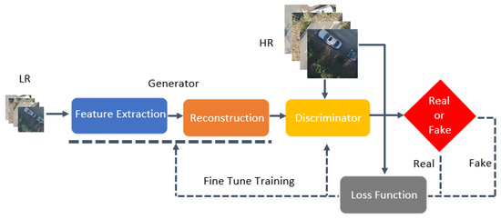
Figure 1.
GAN architecture.
3.1.1. Generation Network
The generation network can map LR image features to HR space, thereby achieving image SR reconstruction. In the feature extraction module of the generation network, we used multi-level dense connections, SA, and residual connections to improve the network’s feature extraction ability. Specifically, we designed a dense-in-residual dense block with SA (SADRDB) and used densely connected SADRDBs (DCSADRDB) as the main part of the feature extraction module. The generation network G is shown in Figure 2.
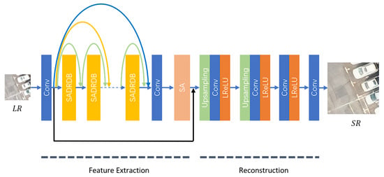
Figure 2.
Generation network architecture.
In the generation network, the LR image is first extracted with shallow features through a 3 × 3 convolution layer. Then, the feature image will pass through the DCSADRDB, which will further extract the deep features of the image. In the DCSADRDB, the input features of each SADRDB are composed of shallow features of the image and the output features of each previous SADRDB, achieving image feature reuse and gradient flow, enhancing the ability to extract deep features of the image. The internal structure of the DCSADRDB can be expressed as
In (2) and (3), is the input feature image of the i-th SADRDB; is the shallow feature image after the first convolution layer; is the residual coefficient [46]; is the output feature image of the i-th SADRDB; is the mapping relationship of the i-th SADRDB.
Then, the network uses a 3 × 3 convolution layer and SA layer of 3 to extract deep features further. SA divides input features into groups, integrating channel and spatial attention into a block for each group. Each group outputs sub-features through this block, and communication and gathering between sub-features complete the attention operations, outputting image features. The output features are fused with shallow features using residual connections. The fused features are amplified through two sets of upsampling layers, and then the final reconstructed SR image is output through two convolution layers.
The feature extraction module of G includes 23 densely connected SADRDBs for extracting deep features of images. The internal structure of an SADRDB is shown in Figure 3a.
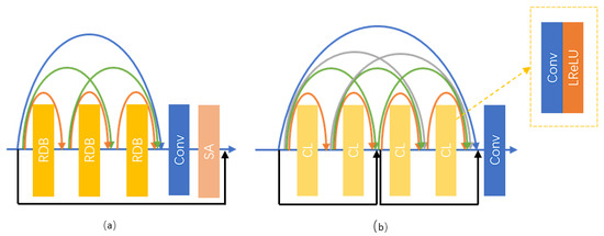
Figure 3.
(a) The internal structure of SARRDB, (b) the internal structure of RDB.
Each SADRDB consists of three residual dense blocks (RDBs), a convolution layer, and an SA layer. The three RDBs are connected by a dense connection, ensuring more efficient utilization of the feature information of each RDB. Finally, residual connections are used to output the features. The internal structure of the i-th SADRDB can be expressed as
In (4)–(8), is the input feature image of the j-th RDB; is the output feature image of the j-th RDB; is the mapping relationship of the j-th RDB; is the feature image output through convolution layers; is the mapping relationship of the convolution layers; is the feature image output through the SA layer; is a mapping relationship of SA.
The structure of the RDB is shown in Figure 3b and consists mostly of four densely connected convolution and LReLU (CL) layers. Additional residual connections have been added to the RDB to increase network capacity without increasing network complexity [30]. The internal structure of the j-th RDB in the i-th SADRDB can be expressed as
In (9)–(11), is the input feature image of the k-th CL layer; is the output feature image of the k-th CL layer; is a tensor’s Concat operation; is the mapping relationship of the k-th CL layer; is the output of the j-th RDB.
In both the SADRDB and the main structure of the generation network, efficient SA is used, which uses Shuffle Units to effectively combine spatial attention and channel attention to capture pixel-level channel and spatial relationships [47]. The internal structure of SA is shown in Figure 4.
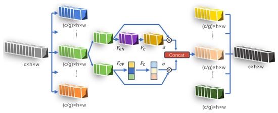
Figure 4.
The internal structure of SA, where c is the number of channels, h is the height, w is the width, and g is the number of groups.
SA divides the input feature map into g groups, each using channel and spatial attention to extract sub-features. Then, all sub-features are aggregated, and the “channel shuffle” operator [48] is used to achieve information communication between different sub-features. The formula for grouping input feature images can be expressed as
In (12), c, h, and w, respectively, represent the number of channels, height, and width of the feature image; g is the number of groups; X is the input feature image of the SA layer; is the feature image of group k.
After grouping, each group needs to pass through channel attention and spatial attention. Each channel of the feature image captures different feature information in the image, which can contain various information such as information about edges, textures, and colors. Through the channel attention mechanism, the network can automatically learn weights to determine the importance of each channel [49]. The channel attention can be expressed as
In (13), is the channel attention output of group k; is the mapping relationship of the Global Average Pooling (GP); is a linear transformation; is the sigmoid transformation.
The spatial attention mechanism is used to enhance the attention level of neural networks to different spatial positions in input data. This attention mechanism allows the network to dynamically learn the attention weights that should be assigned at different positions [50] in order to handle tasks better. The spatial attention formula is as follows:
In (14), is the spatial attention output of group k; is the mapping relationship of the Group Norm (GN) [51].
Subsequently, each group’s channel and spatial attention output are connected, and the outputs of each group are aggregated. The “channel shuffle” operator is used to achieve the flow of cross-group information along the channel dimension. SA is a lightweight, plug-and-play module that can be used to improve the network’s ability to extract features.
3.1.2. Discrimination Network
The classic VGG-style discrimination network passes the input image through several convolution layers and a fully linked layer and then judges the distribution difference between and through the entire image region, which is also one of the reasons why the method of using VGG-style discrimination network is not sensitive to local texture details [52]. The VGG-style discrimination network makes it difficult for the network to recover realistic texture details in feature-rich local areas. Therefore, we propose a PatchGAN-style discrimination network. It is a complete convolutional topology network without fully connected layers. Its core idea is to divide the input image into multiple small patches and independently distinguish each small block. Due to the independent processing of each small block, this discrimination network allows the model to focus more on local structure and details rather than global consistency. The output result is an matrix, where each point represents a small area of the original image indicating the likelihood that each area is an actual sample, as shown in Table 1. The final result of the discrimination network is the average evaluation of these regions. PatchGAN-style discrimination networks have advantages in generating more realistic texture details [53]. The internal structure of the discrimination network is shown in Figure 5.

Table 1.
The size of the receptive field of each convolution layer of the discrimination network, where l is the size of the input image, k is the size of the convolution kernel, p is the filling amount, s is the size of the convolution step, and n is the size of the output matrix representing the receptive field.

Figure 5.
Discrimination network architecture.
3.2. Loss Functions
3.2.1. Pixel Loss
Pixel loss calculates the difference between two images on a pixel-by-pixel basis. Therefore, the image SR reconstruction method can judge the consistency of the SR and HR images at the pixel level through pixel loss. The formula for pixel loss is as follows:
In (15), and are the feature image of paired LR and HR images in the dataset, M is the number of pairs in the dataset, and is the mapping relationship between and in the generation network.
3.2.2. Perception Loss
The perceptual loss function can calculate the difference in high-level feature representation between the generated and HR images, solving the problem of weak pixel loss in supervising high-frequency features. It can better represent the image texture information by using high-frequency feature mapping to calculate the perceptual loss before the activation layer in the perceptual network (usually the VGG network), allowing the network to generate more realistic textures [28]. The formula for perceived loss is as follows:
In (16), is the dimension of feature images in the VGG network; is the feature image of LR remote sensing images; is the feature image of HR remote sensing images; . ) is the mapping relationship before the j-th convolution layer and i-th maximum pooling layer in layer 19 of the VGG network.
3.2.3. Adversarial Loss
The adversarial loss can help the generation network and the discrimination network to conduct adversarial training, helping the network to generate higher-quality images. The formula for adversarial loss is as follows:
In (17)–(19), is the matrix output by through discrimination network D; is the output matrix of after passing through discrimination network D; is the sigmoid function, which converts the matrix obtained from the difference into a probability matrix between 0 and 1; and are obtained through matrix transformation. Formula (19) indicates that the optimization objective for each element in the matrix is 0, and the optimization objective for each element in the matrix is 1. Supervising adversarial losses can make the images generated by the generation network more realistic, allowing the discrimination network to determine whether the images are authentic more accurately [54].
3.2.4. Artifact Loss
GANs have the potential to generate rich and detailed clear images, but, due to the dynamicity of adversarial training, unpleasant artifacts are often generated [55]. Texture details and artifacts often occur in the high-frequency feature areas of the image [41]. While the model’s ability to generate texture details is enhanced, the impact of artifacts on the image is also enhanced. To solve this problem, we use the artifact loss function [56] for optimization.
Firstly, we calculate the residual of and as follows:
Subsequently, local statistics are calculated to determine the pixel differences within a certain area. The formula can be expressed as
In (21), n is the statistical area size; is calculating the variance of pixels in the region. Local statistics can better identify texture details with regular edges, but their recognition effect on texture details with random distribution is poor. Therefore, we use a global patch N to solve this problem, and the formula is as follows:
In (22), is a global patch parameter. We use to identify the artifact region. However, in the early stages of adversarial training, there are still certain recognition errors, leading to excessive punishment for realistic texture details. To solve this problem, we use the EMA technique [57] with the following formula:
In (23), is the weight parameter; k is the number of network iterations; is the model obtained through training for the k-th time; and is the model obtained through the EMA technique. Compared with , is more reliable and can reduce the generation of random artifacts.
We use EMA technology to optimize , as shown in Figure 6. After obtaining and in each iteration, these two models use to generate and and then calculate the residuals to obtain and . determines the penalty position by comparing and , and, finally, is multiplied by to obtain the final artifact loss. The calculation process can be expressed as Formulas (24)–(26):
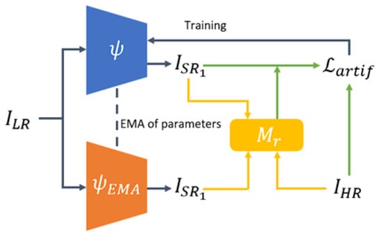
Figure 6.
Training process combining EMA technology.
3.2.5. Total Loss
The total loss combines the five losses mentioned above and can be expressed as
In (27), are the coefficients of each loss; is the pixel loss; is the perceived loss; is the adversarial loss; is the artifact loss.
4. Experiments and Results
This experiment was implemented on the Pytorch framework using a GTX3060 12G GPU. The batch size of the experimental input image was set to 16. We randomly cropped the HR image to and the LR image to 32 × 32. In Guo’s experiment, it was proven that the network performance is best when the residual coefficient is 0.2 [58]; therefore, our model’s residual coefficient is set to 0.2. In Liang’s experiment, it was proved that setting the weight parameter of EMA to 0.999 can effectively improve the stability of model training [56]; therefore, our EMA weight parameter was set to 0.999. Loss function coefficient , , , . In the subsequent ablation experiments, we will also discuss the impact of the weight of the artifact loss function on the model. The number of training iterations was set to . The initial learning rate was set to . The Adam optimizer of the generation network and discrimination network was set to , .
4.1. Dataset
We used the RHLAI dataset [58] for our experiment, which includes images of surface landscapes in Yichang City, Hubei Province, China, such as farmland, houses, roads, and forests. The researcher obtained remote sensing images with resolutions of 0.2 m and 0.5 m by processing aerial photography, and then processed them into 9288 pairs of HR images with a pixel size of 256 × 256 and LR images with a pixel size of 64 × 64. We divided the HR and LR images into training, evaluation, and testing datasets in an 8:1:1 ratio. Figure 7 shows some high-definition images from this dataset.
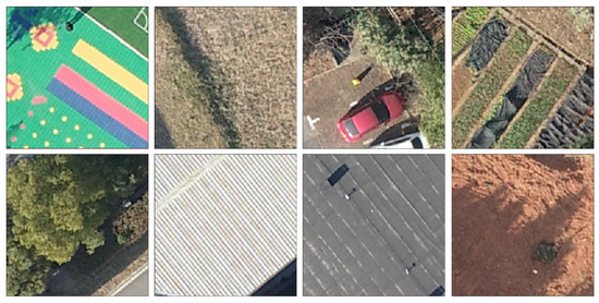
Figure 7.
Some images from the RHLAI dataset.
Most of the datasets for remote sensing image SR reconstruction only have HR remote sensing images. Researchers often use the downsampling method to reduce the HR images to obtain the LR images. There is a certain mathematical relationship between them. In the application scenario of remote sensing images, the observed remote sensing images are usually used as the original data to obtain HR images which are somewhat different from the LR images reduced by the downsampling method in experiments. Therefore, our experiments used the RHLAI dataset, which uses observed remote sensing images as LR images and can better reflect the reconstruction performance in practical applications. In the experiment of Guo et al. [58], the feasibility of this dataset was demonstrated.
4.2. Evaluation Metrics
In this research, three evaluation indicators of image SR reconstruction methods, peak signal-to-noise ratio (PSNR), structural similarity (SSIM) [59], and learning perception image patch similarity (LPIPS) [60], were selected to evaluate the experimental results. PSNR can be used to calculate the pixel difference between the SR reconstructed image and the HR image. The calculation formula for PSNR is as follows:
SSIM can evaluate the structural similarity between the SR reconstructed image and the HR image, paying more attention to the local structural differences. The SSIM calculation formula is as follows:
In (30), and are the pixel mean of image x and y; is the covariance of images x and y; and are the variance corresponding to images x and y; and are the non-zero constants.
LPIPS is an evaluation metric for comparing features extracted by deep learning networks which can better represent the human eye’s perception of image quality. Compared with traditional evaluation indicators, LPIPS is more advantageous in assessing human visual perception of images [60]. It can be obtained by calculating the image distance , which can be expressed as the following formula (31):
4.3. Analysis of Image Quality Metrics during Training Process
During our model training process, we saved model weights every 10,000 iterations and validated metrics such as PSNR, SSIM, and LPIPS and plotted them into line graphs as shown in Figure 8.

Figure 8.
(a) PSNR line graphs plotted during TDEGAN training; (b) SSIM line graphs plotted during TDEGAN training; (c) LPIPS line graphs plotted during TDEGAN training.
Figure 8a shows the changes in the PSNR of TDEGAN during training. It can be seen that, in the initial stages of training, the PSNR volatility of the images generated by the model increases. Subsequently, the model oscillates within a specific range, with an oscillation amplitude of around 0.6, indicating that our model is still learning the image features of the dataset. In the later stage of training, our model gradually stabilizes at an amplitude of around 0.2, indicating that our model gradually converges.
Figure 8b shows the changes in SSIM during TDEGAN training. Like the metric shown in Figure 8a, SSIM rapidly rises in the initial stages of model training and oscillates over an extensive range, with an amplitude of around 0.02. In the later stage of training, the range of SSIM changes gradually decreases, and the model begins to converge with an amplitude of around 0.01.
Figure 8c shows the changes in LPIPS during TDEGAN training. In the initial stage of training, LPIPS rapidly decreases, followed by an extensive range of oscillations with an oscillation range of around 0.03. Subsequently, the oscillation range gradually decreases, and, in the later stage of model training, the amplitude is around 0.01, and the model gradually stabilizes.
4.4. Comparative Experiment
We chose bicubic interpolation, SRCNN [20], EDSR [24], SRGAN [27], ESRGAN [29], SPSR [61], and SAM-DiffSR [62] methods for comparative experiments conducted with TDEGAN in the same experimental environment.
Table 2 shows the indicator sizes tested by different methods on the test dataset. Compared to methods based on other methods, the bicubic interpolation and CNN-based methods have certain advantages in the PSNR and SSIM metrics. However, PSNR focuses more on pixel differences, while SSIM focuses on three indicators, brightness, contrast, and structure, which cannot effectively represent perceptual quality. In the experiment of Wang et al. [29], it was also pointed out that PSNR-guided methods are prone to producing ambiguous results. LPIPS is an indicator used to measure image similarity, which is closer to the perception of the human visual system. In Guo et al.’s experiment [58], it was also shown that bicubic interpolation methods and CNN-based methods are more inclined to generate blurred images with higher PSNR and SSIM values, while GAN-based methods, although they have lower PSNR and SSIM, have better visual perception quality and higher LPIPS values. Therefore, we introduced LPIPS indicators that better reflect human visual perception to evaluate the reconstruction effects of each method. Table 2 shows that our model has the best LPIPS metric, indicating that the reconstructed images of our model have better visual perception effects. Of course, our model also has certain advantages regarding the PSNR and SSIM metrics among other methods.

Table 2.
The best PSNR, SSIM, and LPIPS values obtained using different methods on the RHLAI test dataset are represented in bold. Especially for other methods, the best values are represented by underscores.
From Figure 9, we can see that we selected features such as roofs, farmland, vehicles, and roads for visual comparison. Overall, the images reconstructed by bicubic interpolation, SRCNN, and EDSR methods are relatively blurry, and the effect of reconstructing texture details is poor. In contrast, other methods have certain advantages. The first row of roof images shows that the images reconstructed by SRGAN and SPSR methods have specific texture details. However, the roof lines are blurry and discontinuous. The image lines reconstructed by the ESRGAN method are relatively straightforward and complete. However, it can be seen that there are some artifacts around the lines, which affect the visual effect. The SAM-DiffSR method has a good reconstruction effect, but the roof lines are not smooth and natural. Our method reconstructs images with clear and complete roof lines, providing the best visual effect. The farmland image in the second row shows that the texture effect of the images reconstructed by SRGAN and SPSR methods can be poor, lacking the expression of farmland gully features, and the specific details of the image cannot be clearly seen. The ESRGAN method reconstructs relatively smooth and somewhat blurry images after local magnification. The farmland gullies reconstructed by the SAM-DiffSR method are relatively clear and complete, but some details are missing. Our method reconstructs images of farmland gullies with clear texture, complete lines, and flat edges. The third line of the image contains cars on the road, and the textures on both sides of the car reconstructed using SRGAN, ESRGAN, and SAM-DiffSR methods are relatively blurry. The car images reconstructed using the SPSR method have some artifacts that affect the visual effect. The texture of the car image reconstructed by our model is natural and realistic, clearly showing the car’s local details and overall structure. The fourth and fifth lines of images show that, when reconstructing the lines on the road, there is often generation of artifacts, resulting in unclear edges and poor visual effects of the image features. Our method dramatically reduces the impact of artifacts and increases the clarity of the edges of the ground objects.
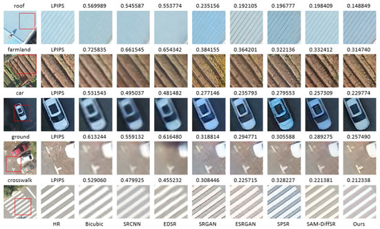
Figure 9.
Comparison of visualization effects and image LPIPS of different SR methods with the original image from the RHLAI test dataset on the far left and locally enlarged images on the other side.
The above indicates that our model has certain advantages over some classic models in terms of indicators and visual effects as it can reduce the impact of artifacts and generate images with better texture details.
4.5. Ablation Experiment
In order to systematically demonstrate the improvement of our model generation network, discrimination network, and loss function on model performance, we conducted ablation experiments using the following networks: (a). baseline (ESRGAN), (b). baseline + DCSADRDB, (c). baseline + DCSADRDB + PatchGAN-style discrimination network, (d). DCSADRDB + PatchGAN-style discrimination network + artifact loss (TDEGAN). We trained the above networks under the same conditions and tested the test dataset, as well as calculated the PSNR, SSIM, and LPIPS indicators.
Table 3 shows that the LPIPS indicators in each module gradually added to the baseline network improve to some extent. Especially for the LPIPS indicator, which can better reflect human visual perception, our final improved model is 0.017024, smaller than the baseline model. This indicates that modules such as the DCSADRDB, PatchGAN-style discrimination network, and artifact loss function can effectively improve the ability to generate better perceptual images. Figure 10 compares the visualization effects of three types of land features: farmland, roof, and playground. The network’s reconstruction effect on texture details is enhanced with the introduction of the modules. From the farmland in the first row, it can be seen that, after the introduction of the DCSADRDB, the image details become more abundant, and the gullies in the farmland gradually become clear. From the texture of the second row of the roof, it can be seen that the roof lines gradually become more three-dimensional and better reflected in visual perception. However, the impact of artifacts also increases. When we introduce artifact loss, the problem of generating artifacts is significantly reduced. From the lines on the playground, it can be seen that the clarity of the image gradually improves. After introducing the PatchGAN-style discrimination network, there are black artifacts on both sides of the white lines on the playground. After improving the loss function, TDEGAN not only enhances the clarity of the lines but also reduces the impact of artifacts around the lines. From this, we can see that our various modules improve the indicators. In terms of visual effects, combining each module enhances details and image clarity and counters the impact of artifacts.

Table 3.
The best PSNR, SSIM, and LPIPS values from different networks tested on the RHLAI test dataset are represented in bold in the ablation experiment.
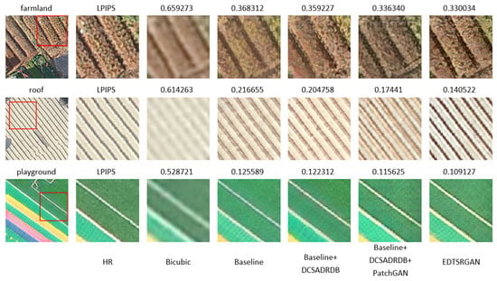
Figure 10.
Comparison of visualization effects and image LPIPS of each network with the original image of the test RHLAI dataset on the far left and locally enlarged images on the other side.
In order to improve the performance of the generator, we added multi-level dense connections and additional residual connections to the generation network, forming a multi-level dense connection network (DCDRDB). In order to further improve the feature extraction performance, SA modules were added to the generative network to form a DCSADRDB. We used an RRDB as the baseline generation network and conducted ablation experiments on the above two improvements.
As shown in Table 4, with the continuous improvement of our generated network, all the tested indicators gradually improve. The PSNR index increases by about 0.3. SSIM increases by about 0.018. LPIPS increases by about 0.01. As shown in Figure 11, as our generative network improves, the visualization effect of the generated images gradually improves. When the generated network is the RRDB, the details of the car windows and nearby grass are unclear, the edges of the lines on the road are blurry, and the texture of the roof of the house is poor. When the generation network is a DCDRDB, the details of the generated image are more abundant. When the generation network is a DCSADRDB, as the network’s feature extraction ability improves, the visual effect of the image also further improves. The texture details of the car and grass become richer and more realistic, the lines on the road are clearer, and the stripes on the roof of the house are closer to those of the HR image.

Table 4.
The best PSNR, SSIM, and LPIPS values for different generation networks tested on the RHLAI test dataset are represented in bold for the ablation experiment.
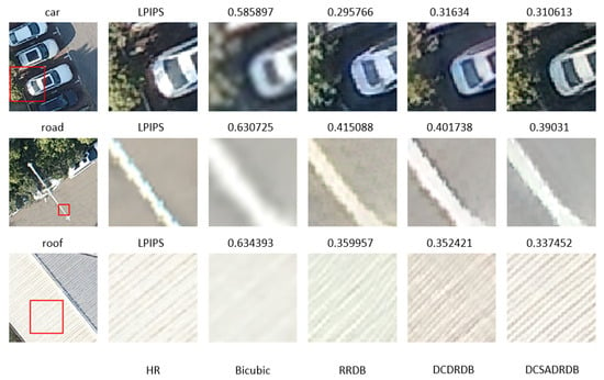
Figure 11.
Comparison of visualization effects and image LPIPS of each generation network with the original image of the test RHLAI dataset on the far left and locally enlarged images on the other side.
A GAN has the potential to generate rich and detailed clear images but often produces unpleasant artifacts. While the model’s ability to generate texture details is enhanced, the impact of artifacts on the image is also enhanced. To solve this problem, we used the artifact loss function for optimization. To further explore the effectiveness of the artifact loss function, we set the weights of the artifact loss function to 0.5, 1, and 1.5 for the ablation experiments.
The artifact loss function can distinguish between artifacts and real texture details through local statistics, and help the network generate better images by punishing artifacts. The weight L of the artifact loss can control the penalty intensity of the loss function on the artifact area. From Table 5, we can see that, when L is 1, the PSNR, SSIM, and LPIPS are the best indicators. When L is 0.5, the penalty for the loss function is insufficient, and the optimal effect is not achieved. When L is 1.5, the penalty of the loss function is excessive, and, due to the often simultaneous generation of artifacts and real textures, it has an impact on the real texture, resulting in a deterioration of the indicator effect. From Figure 12, it can be seen that, when L is 0.5, there are certain artifacts in the texture of the car, the lines on the road, and the patterns on the playground, which affect the visual effect. When L is 1, the artifacts are greatly reduced, the lines become clearer, the texture details are more realistic, and the visual effect of the image is the best. When L is 1.5, although the effect of artifacts in the image is reduced, texture details are also reduced, and local areas become blurred. So, in our model, the weight selection for artifact loss is 1.

Table 5.
The best PSNR, SSIM, and LPIPS values achieved using different loss weights on the RHLAI test dataset are represented in bold for the ablation experiment.
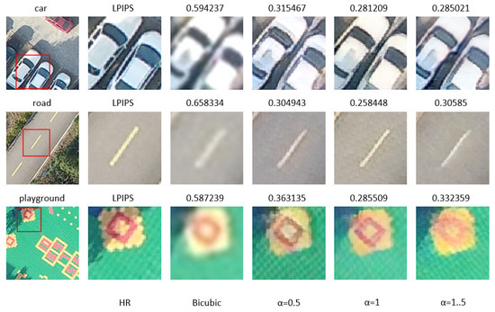
Figure 12.
Comparison of visualization effects and image LPIPS of each loss weight with the original image of the test RHLAI dataset on the far left and locally enlarged images on the other side.
5. Discussion
NWPU-RESSC45 contains large-scale remote sensing images of various scenes with significant differences and has a certain representativeness. The images in the dataset were randomly divided into three parts in an 8:1:1 ratio to provide training, inference, and testing for the models. We tested the metrics for the images in five different scenarios, as shown in Table 6.

Table 6.
The best PSNR, SSIM, and LPIPS values achieved using different methods on the NWPU-RESISC45 test dataset are represented in bold. In other methods, the best values are represented by underscores.
As mentioned, methods based on bicubic interpolation and CNNs tend to achieve higher PSNR and SSIM metrics. However, in terms of visual perception, LPIPS is more representative of the reconstruction quality of images. Our model achieved the best LPIPS metrics in image reconstruction for all five scenarios, and the highest PSNR and SSIM metrics were achieved by other methods. Figure 13 shows the visualization comparison of different methods tested on the NWPU-RESISC45 test dataset. Our method had better visualization performance. This further demonstrates that our model has certain advantages in reconstructing remote sensing images.
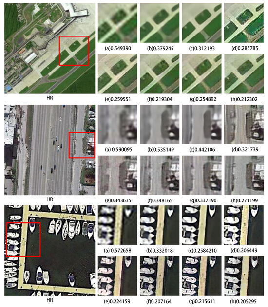
Figure 13.
Visualization comparison and LPIPS indicators of different methods tested on the NWPU-RESISC45 test dataset: (a) bicubic, (b) SRCNN, (c) EDSR, (d) SRGAN, (e) ESRGAN, (f) SPSR, (g) SAM-DiffSR, (h) ours.
6. Conclusions
Image SR reconstruction technology has been widely used in the application of remote sensing images. Image SR reconstruction technology based on GANs has attracted attention due to its ability to generate more explicit images. However, generating more realistic texture details and reducing image artifacts remain challenges. To address these challenges, we propose TDEGAN.
We propose DCSADRDB as the main part of the generation network which adds multi-level dense-connection SA and residual connections to improve the feature extraction capability of the network. We design a PatchGAN-style discrimination network instead of the classic VGG-style discrimination network which can perform local discrimination and help the generation network generate more rich texture details. However, while enhancing the model’s ability to generate texture details, it often generates some unpleasant artifacts. To solve this problem, we introduce artifact loss, which combines with EMA technology to calculate local statistics to distinguish between realistic details and artifacts, thereby helping the network generate more realistic texture details and reducing the impact of artifacts. Compared with existing methods, our model can generate more realistic texture details, reconstruct higher image quality, and achieve better visual perception and evaluation indicators.
Although our model demonstrated certain performance advantages when tested on the RHLAI and NWPU-RESISC45 datasets, there is also the problem of enhancing the universality of the model. How to train models that can be applied to more remote sensing datasets and enhance the universality of SR reconstruction models for remote sensing images remains one of the challenges to be solved in the future.
Author Contributions
M.G. and F.X. designed the TDEGAN architecture and conducted comparative and ablation experiments. B.Z., Y.H., L.W. and Z.X. analyzed and summarized the experimental results, data, and visualization images. M.G. and F.X. wrote this manuscript. B.Z., Y.H., L.W., Z.X., X.C. and J.Z. provided reliable suggestions during the paper revision process. All authors have read and agreed to the published version of the manuscript.
Funding
This work was funded by the National Natural Science Foundation of China (41971356, 41701446) and the Open Fund of Key Laboratory of Urban Land Resources Monitoring and Simulation, Ministry of Natural Resources.
Data Availability Statement
No new datasets were created or analyzed.
Conflicts of Interest
Baorui Zhao is empoyed by Hubei Geomatics Technology Group Stock Co., Ltd., Ying Huang is empoyed by Wuhan Zondy Cyber Technology Co., Ltd. The remaining authors declare that the research was conducted in the absence of any commercial or financial relationships that could be construed as a potential conflict of interest.
References
- Wang, Z.; Jiang, K.; Yi, P.; Han, Z.; He, Z. Ultra-dense GAN for satellite imagery super-resolution. Neurocomputing 2020, 398, 328–337. [Google Scholar] [CrossRef]
- Lim, S.B.; Seo, C.W.; Yun, H.C. Digital Map Updates with UAV Photogrammetric Methods. J. Korean Soc. Surv. Geod. Photogramm. Cartogr. 2015, 33, 397–405. [Google Scholar] [CrossRef][Green Version]
- Guo, M.; Liu, H.; Xu, Y.; Huang, Y. Building Extraction Based on U-Net with an Attention Block and Multiple Losses. Remote Sens. 2020, 12, 1400. [Google Scholar] [CrossRef]
- Sun, H.; Sun, X.; Wang, H.; Li, Y.; Li, X. Automatic Target Detection in High-Resolution Remote Sensing Images Using Spatial Sparse Coding Bag-of-Words Model. IEEE Geosci. Remote Sens. Lett. 2012, 9, 109–113. [Google Scholar] [CrossRef]
- Xia, L.; Zhang, X.; Zhang, J.; Wu, W.; Gao, X. Refined extraction of buildings with the semantic edge-assisted approach from very high-resolution remotely sensed imagery. Int. J. Remote Sens. 2020, 41, 8352–8365. [Google Scholar] [CrossRef]
- Yokoya, N.; Grohnfeldt, C.; Chanussot, J. Hyperspectral and Multispectral Data Fusion: A comparative review of the recent literature. IEEE Geosci. Remote Sens. Mag. 2017, 5, 29–56. [Google Scholar] [CrossRef]
- Cui, K.; Li, R.; Polk, S.L.; Lin, Y.; Zhang, H.; Murphy, J.M.; Plemmons, R.J.; Chan, R.H. Superpixel-Based and Spatially Regularized Diffusion Learning for Unsupervised Hyperspectral Image Clustering. IEEE Trans. Geosci. Remote Sens. 2024, 62, 1–18. [Google Scholar] [CrossRef]
- Wang, P.; Sertel, E. Channel-spatial attention-based pan-sharpening of very high-resolution satellite images. Knowl.-Based Syst. 2021, 229, 107324. [Google Scholar] [CrossRef]
- Koester, E.; Sahin, C.S. A Comparison of Super-Resolution and Nearest Neighbors Interpolation Applied to Object Detection on Satellite Data. arXiv 2019, arXiv:1907.05283. [Google Scholar]
- Xiang-guang, Z. A New Kind of Super-Resolution Reconstruction Algorithm Based on the ICM and the Bicubic Interpolation. In Proceedings of the 2008 International Symposium on Intelligent Information Technology, Shanghai, China, 21–22 December 2008; pp. 817–820. [Google Scholar]
- Xiang-guang, Z. A New Kind of Super-Resolution Reconstruction Algorithm Based on the ICM and the Bilinear Interpolation. In Proceedings of the 2008 International Seminar on Future BioMedical Information Engineering, Wuhan, China, 18 December 2008; pp. 183–186. [Google Scholar]
- Rasti, P.; Demirel, H.; Anbarjafari, G. UIterative Back Projection based Image Resolution Enhancement. In Proceedings of the 2013 8th Iranian Conference on Machine Vision and Image Processing (MVIP), Zanjan, Iran, 10–12 September 2013; pp. 237–240. [Google Scholar]
- Schultz, R.; Stevenson, R. Extraction of high-resolution frames from video sequences. IEEE Trans. Image Process. 1996, 5, 996–1011. [Google Scholar] [CrossRef] [PubMed]
- Stark, H.; Oskoui, P. High-Resolution Image Recovery from Image-Plane Arrays, Using Convex Projections. J. Opt. Soc. Am. A-Opt. Image Sci. Vis. 1989, 6, 1715–1726. [Google Scholar] [CrossRef]
- Xu, J.; Gao, Y.; Xing, J.; Fan, J.; Gao, Q.; Tang, S. Two-direction self-learning super-resolution propagation based on neighbor embedding. Signal Process. 2021, 183, 108033. [Google Scholar] [CrossRef]
- Zhang, J.; Shao, M.; Yu, L.; Li, Y. Image super-resolution reconstruction based on sparse representation and deep learning. Signal Process.-Image Commun. 2020, 87, 115925. [Google Scholar] [CrossRef]
- Yao, T.; Luo, Y.; Chen, Y.; Yang, D.; Zhao, L. Single-Image Super-Resolution: A Survey. In Proceedings of the 2018 CSPS Volume II: Signal Processing; Springer: Singapore, 2020; pp. 119–125. [Google Scholar]
- Bashir, S.M.A.; Wang, Y.; Khan, M.; Niu, Y. A comprehensive review of deep learning-based single image super-resolution. PeerJ Comput. Sci. 2021, 232, 621. [Google Scholar] [CrossRef] [PubMed]
- Wang, Z.; Chen, J.; Hoi, S.C.H. Deep Learning for Image Super-Resolution: A Survey. IEEE Trans. Pattern Anal. Mach. Intell. 2021, 43, 3365–3387. [Google Scholar] [CrossRef] [PubMed]
- Dong, C.; Loy, C.C.; He, K.; Tang, X. Image Super-Resolution Using Deep Convolutional Networks. IEEE Trans. Pattern Anal. Mach. Intell. 2016, 38, 295–307. [Google Scholar] [CrossRef]
- Dong, C.; Loy, C.C.; Tang, X. Accelerating the Super-Resolution Convolutional Neural Network. In Proceedings of the 14th European Conference, Amsterdam, The Netherlands, 11–14 October 2016; pp. 391–407. [Google Scholar]
- Xu, L.; Ren, J.S.J.; Liu, C.; Jia, J. Deep Convolutional Neural Network for Image Deconvolution. In Advances in Neural Information Processing Systems 27 (NIPS 2014); IEEE: New York, NY, USA, 2014; pp. 1905–1914. [Google Scholar]
- Kim, J.; Lee, J.K.; Lee, K.M. Deeply-Recursive Convolutional Network for Image Super-Resolution. In Proceedings of the IEEE Conference on Computer Vision and Pattern Recognition (CVPR), Las Vegas, NV, USA, 27–30 June 2016; pp. 1637–1645. [Google Scholar]
- Lim, B.; Son, S.; Kim, H.; Nah, S.; Lee, K.M. Enhanced Deep Residual Networks for Single Image Super-Resolution. In Proceedings of the IEEE Conference on Computer Vision and Pattern Recognition (CVPR) Workshops, Honolulu, HI, USA, 21–26 July 2017; pp. 1132–1140. [Google Scholar]
- He, K.; Zhang, X.; Ren, S.; Sun, J. Deep Residual Learning for Image Recognition. In Proceedings of the IEEE Conference on Computer Vision and Pattern Recognition (CVPR), Las Vegas, NV, USA, 27–30 June 2016; pp. 770–778. [Google Scholar]
- Ju, C.; Su, X.; Yang, H.; Ning, H. Single-image super-resolution reconstruction via generative adversarial network. In Proceedings of the 9th International Symposium on Advanced Optical Manufacturing and Testing Technologies: Optoelectronic Materials and Devices for Sensing and Imaging, Chengdu, China, 26–29 June 2018; Volume 10843, p. 108430. [Google Scholar]
- Ledig, C.; Theis, L.; Huszar, F.; Caballero, J.; Cunningham, A.; Acosta, A.; Aitken, A.; Tejani, A.; Totz, J.; Wang, Z.; et al. Photo-Realistic Single Image Super-Resolution Using a Generative Adversarial Network. In Proceedings of the IEEE Conference on Computer Vision and Pattern Recognition, Honolulu, HI, USA, 21–26 July 2017; pp. 105–114. [Google Scholar]
- Johnson, J.; Alahi, A.; Fei-Fei, L. Perceptual Losses for Real-Time Style Transfer and Super-Resolution. In Proceedings of the 14th European Conference, Amsterdam, The Netherlands, 11–14 October 2016; Volume 9906, pp. 694–711. [Google Scholar]
- Wang, X.; Yu, K.; Wu, S.; Gu, J.; Liu, Y.; Dong, C.; Qiao, Y.; Loy, C.C. ESRGAN: Enhanced Super-Resolution Generative Adversarial Networks. In Proceedings of the European Conference on Computer Vision (ECCV) Workshops, Munich, Germany, 8–14 September 2018; pp. 63–79. [Google Scholar]
- Rakotonirina, N.C.; Rasoanaivo, A. ESRGAN plus: Further Improving Enhanced Super-Resolution Generative Adversarial Network. In Proceedings of the 2020 IEEE International Conference on Acoustics, Speech, and Signal Processing, Virtual, 4–9 May 2020; pp. 3637–3641. [Google Scholar]
- Wang, X.; Xie, L.; Dong, C.; Shan, Y. Real-ESRGAN: Training Real-World Blind Super-Resolution with Pure Synthetic Data. In Proceedings of the IEEE/CVF International Conference on Computer Vision, Montreal, BC, Canada, 11–17 October 2021; pp. 1905–1914. [Google Scholar]
- Wang, P.; Bayram, B.; Sertel, E. A comprehensive review on deep learning based remote sensing image super-resolution methods. Earth-Sci. Rev. 2022, 232, 104110. [Google Scholar] [CrossRef]
- Ma, W.; Pan, Z.; Guo, J.; Lei, B. Super-Resolution of Remote Sensing Images Based on Transferred Generative Adversarial NetworkK. In Proceedings of the IGARSS IEEE International Geoscience and Remote Sensing Symposium, Valencia, Spain, 22–27 July 2018; pp. 1148–1151. [Google Scholar]
- Sustika, R.; Suksmono, A.B.; Danudirdjo, D.; Wikantika, K. Generative Adversarial Network with Residual Dense Generator for Remote Sensing Image Super Resolution. In Proceedings of the 2020 International Conference on Radar, Antenna, Microwave, Electronics, and Telecommunications (ICRAMET), Tangerang, Indonesia, 18–20 November 2020; pp. 34–39. [Google Scholar]
- Guo, D.; Xia, Y.; Xu, L.; Li, W.; Luo, X. Remote sensing image super-resolution using cascade generative adversarial nets. Neurocomputing 2021, 443, 117–130. [Google Scholar] [CrossRef]
- Huang, Z.X.; Jing, C.W. Super-Resolution Reconstruction Method of Remote Sensing Image Based on Multi-Feature Fusion. IEEE Acess 2020, 8, 18764–18771. [Google Scholar] [CrossRef]
- Moustafa, M.S.; Sayed, S.A. Satellite Imagery Super-Resolution Using Squeeze-and-Excitation-Based GAN. Int. J. Aeronaut. Space Sci. 2021, 22, 1481–1492. [Google Scholar] [CrossRef]
- Li, Y.; Mavromatis, S.; Zhang, F.; Du, Z.; Sequeira, J.; Wang, Z.; Zhao, X.; Liu, R. Single-Image Super-Resolution for Remote Sensing Images Using a Deep Generative Adversarial Network With Local and Global Attention Mechanisms. IEEE Trans. Geosci. Remote Sens. 2022, 60, 1–24. [Google Scholar] [CrossRef]
- Gao, L.; Sun, H.M.; Cui, Z.; Du, Y.B.; Sun, H.B.; Jia, R.S. Super-resolution reconstruction of single remote sensing images based on residual channel attention. J. Appl. Remote Sens. 2021, 15, 16513. [Google Scholar] [CrossRef]
- Jia, S.; Wang, Z.; Li, Q.; Jia, X.; Xu, M. Multiattention Generative Adversarial Network for Remote Sensing Image Super-Resolution. IEEE Trans. Geosci. Remote Sens. 2022, 60, 1–15. [Google Scholar] [CrossRef]
- Xu, Y.; Luo, W.; Hu, A.; Xie, Z.; Xie, X.; Tao, L. TE-SAGAN: An Improved Generative Adversarial Network for Remote Sensing Super-Resolution Images. Remote Sens. 2022, 14, 2425. [Google Scholar] [CrossRef]
- Guo, X.; Yang, H.; Huang, D. Image Inpainting via Conditional Texture and Structure Dual Generation. In Proceedings of the IEEE/CVF International Conference on Computer Vision, Montreal, BC, Canada, 11–17 October 2021; pp. 14114–14123. [Google Scholar]
- Wang, W.; Zhang, J.; Niu, L.; Ling, H.; Yang, X.; Zhang, L. Parallel Multi-Resolution Fusion Network for Image Inpainting. In Proceedings of the IEEE/CVF International Conference on Computer Vision, Montreal, BC, Canada, 11–17 October 2021; pp. 14539–14548. [Google Scholar]
- Xu, M.; Chen, Y.; Liu, S.; Li, T.H.; Li, G. Structure-transformed Texture-enhanced Network for Person Image Synthesis. In Proceedings of the IEEE/CVF International Conference on Computer Vision, Montreal, BC, Canada, 11–17 October 2021; pp. 13839–13848. [Google Scholar]
- Xu, B.; Wang, N.; Chen, T.; Li, M. Empirical Evaluation of Rectified Activations in Convolutional Network. arXiv 2015, arXiv:1505.00853. [Google Scholar]
- Szegedy, C.; Ioffe, S.; Vanhoucke, V.; Alemi, A.A. Inception-v4, Inception-ResNet and the Impact of Residual Connections on Learning. In Proceedings of the Thirty-First AAAI Conference on Artificial Intelligence, San Francisco, CA, USA, 4–9 February 2017; pp. 4278–4284. [Google Scholar]
- Zhang, Q.L.; Yang, Y.B. SA-NET: Shuffle Attention for Deep Convolutional Neural Networks. In Proceedings of the 2021 IEEE International Conference on Acoustics, Speech and Signal Processing, Toronto, ON, Canada, 6–11 June 2021; pp. 2235–2239. [Google Scholar]
- Zhang, X.; Zhou, X.; Lin, M.; Sun, R. ShuffleNet: An Extremely Efficient Convolutional Neural Network for Mobile Devices. In Proceedings of the IEEE Conference on Computer Vision and Pattern Recognition, Salt Lake City, UT, USA, 18–23 June 2018; pp. 6848–6856. [Google Scholar]
- Hu, J.; Shen, L.; Albanie, S.; Sun, G.; Wu, E. Squeeze-and-Excitation Networks. IEEE Trans. Pattern Anal. Mach. Intell. 2020, 42, 2011–2023. [Google Scholar] [CrossRef] [PubMed]
- Woo, S.; Park, J.; Lee, J.Y.; Kweon, I.S. CBAM: Convolutional Block Attention Module. In Proceedings of the European Conference on Computer Vision (ECCV), Munich, Germany, 8–14 September 2018; pp. 3–19. [Google Scholar]
- Wu, Y.; He, K. Group Normalization. Int. J. Comput. Vis. 2020, 128, 742–755. [Google Scholar] [CrossRef]
- Isola, P.; Zhu, J.Y.; Zhou, T.; Efros, A.A. Image-to-Image Translation with Conditional Adversarial Networks. In Proceedings of the IEEE Conference on Computer Vision and Pattern Recognition, Honolulu, HI, USA, 21–26 July 2017; pp. 5967–5976. [Google Scholar]
- Zhu, Z.; Lei, Y.; Qin, Y.; Zhu, C.; Zhu, Y. IRE: Improved Image Super-Resolution Based on Real-ESRGAN. IEEE Access 2023, 11, 45334–45348. [Google Scholar] [CrossRef]
- Cheng, J.; Yang, Y.; Tang, X.; Xiong, N.; Zhang, Y.; Lei, F. Generative Adversarial Networks: A Literature Review. KSII Trans. Internet Inf. Syst. 2020, 14, 4625–4647. [Google Scholar]
- Zhao, Z.; Sun, Q.; Yang, H.; Qiao, H.; Wang, Z.; Wu, D.O. Compression artifacts reduction by improved generative adversarial networks. Eurasip J. Image Video Process. 2019, 2019, 1–7. [Google Scholar] [CrossRef]
- Liang, J.; Zeng, H.; Zhang, L. Details or Artifacts: A Locally Discriminative Learning Approach to Realistic Image Super-Resolution. In Proceedings of the IEEE/CVF Conference on Computer Vision and Pattern Recognition, New Orleans, LA, USA, 18–24 June 2022; pp. 5647–5656. [Google Scholar]
- Karras, T.; Laine, S.; Aila, T. A Style-Based Generator Architecture for Generative Adversarial Networks. IEEE Trans. Pattern Anal. Mach. Intell. 2021, 43, 4217–4228. [Google Scholar] [CrossRef] [PubMed]
- Guo, M.; Zhang, Z.; Liu, H.; Huang, Y. NDSRGAN: A Novel Dense Generative Adversarial Network for Real Aerial Imagery Super-Resolution Reconstruction. Remote Sens. 2022, 14, 1574. [Google Scholar] [CrossRef]
- Wang, Z.; Bovik, A.; Sheikh, H.; Simoncelli, E. Image quality assessment: From error visibility to structural similarity. IEEE Trans. Image Process. 2004, 13, 600–612. [Google Scholar] [CrossRef] [PubMed]
- Zhang, R.; Isola, P.; Efros, A.A.; Shechtman, E.; Wang, O. The Unreasonable Effectiveness of Deep Features as a Perceptual Metric. In Proceedings of the IEEE Conference on Computer Vision and Pattern Recognition, Salt Lake City, UT, USA, 18–23 June 2018; pp. 586–595. [Google Scholar]
- Ma, C.; Rao, Y.; Lu, J.; Zhou, J. Structure-Preserving Image Super-Resolution. IEEE Trans. Pattern Anal. Mach. Intell. 2022, 44, 7898–7911. [Google Scholar] [CrossRef] [PubMed]
- Wang, C.; Hao, Z.; Tang, Y.; Guo, J.; Yang, Y.; Han, K.; Wang, Y. SAM-DiffSR: Structure-Modulated Diffusion Model for Image Super-Resolution. arXiv 2024, arXiv:2402.17133. [Google Scholar]
Disclaimer/Publisher’s Note: The statements, opinions and data contained in all publications are solely those of the individual author(s) and contributor(s) and not of MDPI and/or the editor(s). MDPI and/or the editor(s) disclaim responsibility for any injury to people or property resulting from any ideas, methods, instructions or products referred to in the content. |
© 2024 by the authors. Licensee MDPI, Basel, Switzerland. This article is an open access article distributed under the terms and conditions of the Creative Commons Attribution (CC BY) license (https://creativecommons.org/licenses/by/4.0/).