Abstract
Over several decades, high-frequency (HF) radars have been employed for remotely measuring various ocean surface parameters, encompassing surface currents, waves, and winds. Wind direction and speed are usually estimated from both first-order and second-order Bragg-resonant scatter from two or more HF radars monitoring the same area of the ocean surface. This limits the observational domain to the common area where second-order scatter is available from at least two radars. Here, we propose to estimate wind direction and speed from the first-order scatter of a single HF radar, yielding the same spatial coverage as for surface radial currents. Wind direction is estimated using the ratio of the positive and negative first-order Bragg peaks intensity, with a new simple algorithm to remove the left/right directional ambiguity from a single HF radar. Wind speed is estimated from wind direction and de-tided surface radial currents using an artificial neural network which has been trained with in situ wind speed observations. Radar-derived wind estimations are compared with in situ observations in the Lower Saint-Lawrence Estuary (Quebec, Canada). The correlation coefficients between radar-estimated and in situ wind directions range from to for Wellen Radars (WERAs) and from to for Coastal Ocean Dynamics Applications Radars (CODARs), while the root mean square differences range from 8° to 12° for WERAs and from 10° to 19° for CODARs. Correlation coefficients between the radar-estimated and the in situ wind speeds range from to for WERAs and from to for CODARs, while the root mean square differences range from 1.3 m.s−1 to 2.3 m.s−1 for WERAs and from 1.6 m.s−1 to 3.9 m.s−1 for CODARs.
1. Introduction
Remote sensing of sea surface winds holds significant value across various research and commercial applications, including search and rescue, hurricane detection, weather forecasting, sailing, and fishing activities. Traditionally, ocean wind data has been gathered through methods such as ship-anemometers, fixed meteorological stations, moored buoys, or satellite observations. However, each of these methods comes with limitations. Ship-anemometers provide data only along specific routes, while buoys are confined to single positions, necessitating expensive deployments of multiple buoys for wider coverage and frequent maintenance due to the challenging marine environment. Satellite data offer a wide spatial coverage but are costly and offer limited temporal resolution. Therefore, there is a clear need for a cost-effective approach that provides wind data over extensive areas with high temporal resolution. During the last decades, ground-wave high-frequency (HF) radars have been proven to be an effective tool to measure various ocean surface parameters. Unlike conventional microwave radars, the signals from these radars can cover significantly greater distances, because the sea surface is an excellent conductor at HF, facilitating signal propagation.
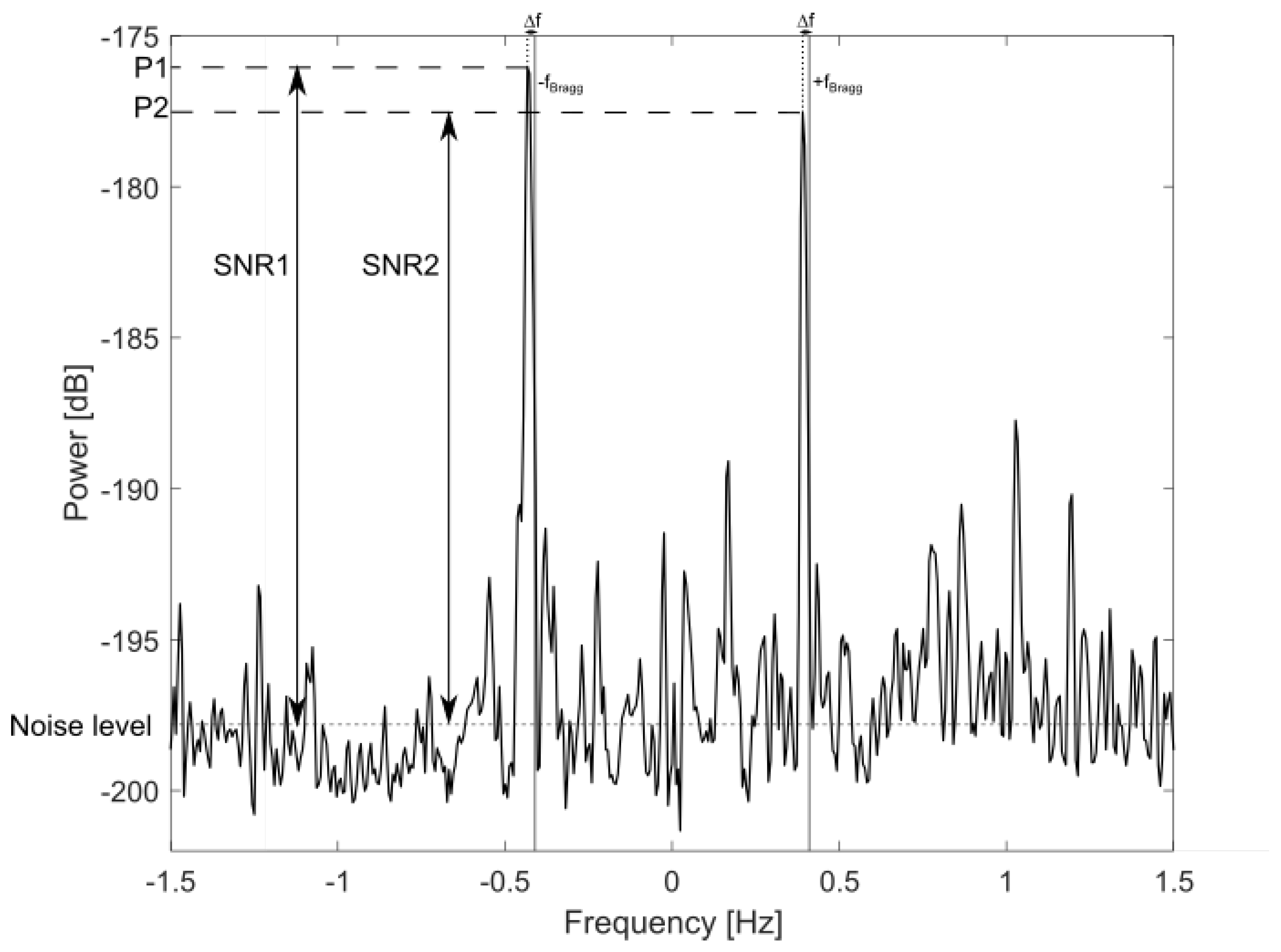
Long and Trizna (1973) [1] is one of the earliest papers involving the estimation of wind from HF backscatter data. In this work, a sky-wave HF radar was employed to collect measurements of wind direction in the Atlantic, using the ratio between positive and negative first-order Bragg peaks. Although this study used a sky-wave HF radar, it initiated numerous studies that focused on extracting wind direction from the first-order Bragg peaks of ground-wave HF radars [2,3,4]. To estimate wind speed, Ahearn et al. (1974) [5] were the first to propose using the ratio of the second-order continuum close to zero Doppler shift to the amplitudes of the first-order Bragg peaks. In this region of the Doppler spectrum, the short waves, which quickly respond to local winds, are responsible for the second-order continuum. Other authors [6,7] proposed using significant wave height and period derived from the second-order sidebands of the radar Doppler spectra. However, the use of the second-order signal reduces coverage due to the lower signal-to-noise ratio, in comparison to using the first-order signal, and may not represent local wind conditions when swell is present. A Doppler spectrum of an HF radar is shown in Figure 1, where the first-order sea echoes are clearly visible, but the second-order echoes do not exhibit a significant elevation above the background noise level. Stewart and Barnum (1975) [8] proposed deriving wind speed from the first-order Bragg peak broadening using HF sky-wave radar data, but this approach has limitations [9].
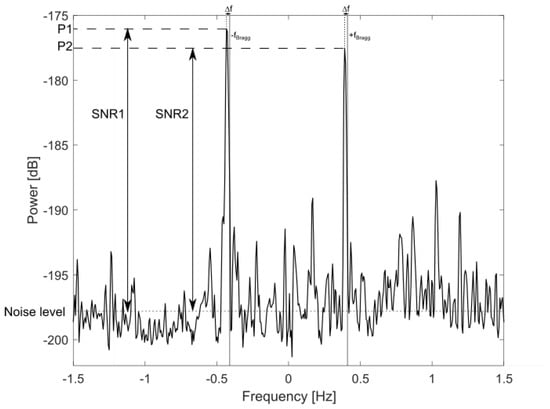
Figure 1.
An example of a HF radar sea echo Doppler spectrum from the WERA W2 (16.15 MHz) showing the first-order Bragg peaks. is the Bragg frequency, and is the offset of the first-order peak relative to the Bragg frequency. The SNR of the first-order peaks are indicated.
Vesecky et al. (2005) [10] proposed a method for estimating wind speed from first-order signals; however, their approach relies on multi-frequency systems to estimate near-surface current shear. Shen et al. (2012) [11] investigated the possibility for wind speed estimation from radar first-order backscatter signals using two different methods. The first method is based on the absolute energy level of first-order radar peaks, while the second method is based on the directional spreading of waves at the Bragg frequency. In both cases, artificial neural network (ANN) analysis is used to establish the relations between pertinent parameters and wind speed. Wen et al. (2020) [12] employed an ANN to develop a statistical model linking the wind-driven current speed measured by HF radars to wind speed. Their approach involved inputting key parameters such as wind direction and the components of wind-driven current estimated from two radars into the neural network. This allowed them to obtain both wind direction and speed with a high degree of accuracy. Recently, Wyatt (2022) [13] employed the support vector machine (SVR) method by utilizing features extracted from the radar Doppler spectrum and metocean parameters linked to wind speed to formulate a wind speed measurement model (refer to Table 3 in [13]). She demonstrated that not all features carry the same weight in the SVR method (see Table 4 in [13]). To simplify the modeling process, she suggested removing features with low or negative importance. However, it is noteworthy that the relative importance of features varies across different sites, resulting in distinct models for each site (see Figure 8 and Table 5 in [13]).
All the previous methods necessitate two or more overlapping radar sites, which limits the spatial coverage. In order to expand the estimation of wind fields to regions covered by a single HF radar, we propose to modify the ANN approach of [12], by utilizing radial currents and wind directions obtained from a single HF radar as the input parameters for the ANN. Consequently, our ANN model comprises two inputs and one output, allowing for effective wind field estimation in areas monitored by a single HF radar. The expression relating wind direction to the first-order spectral peaks is revisited in Section 2. Additionally, Section 2 provides a description of the neural network used to estimate wind speed. Section 3 documents the study area and data. In Section 4, wind fields obtained from real radar data are compared to in situ wind observations from a buoy or meteorological station. Finally, in Section 5, we present a discussion that encompasses an examination of the method’s limitations and offers recommendations for future research directions.
2. Methods
2.1. Wind Direction Estimation by a Single HF Radar
Assuming that the wind direction aligns with the direction of waves exhibiting maximum amplitude (a reasonable assumption for wind waves), it becomes possible to derive the wind direction using the ratio (R) of the power of the two Bragg peaks. To establish a relation between R and the wind direction, the assumption is made that the distribution of surface wave energy, in equilibrium with the local wind, can be modeled as the square of a hyperbolic secant function [11,14]
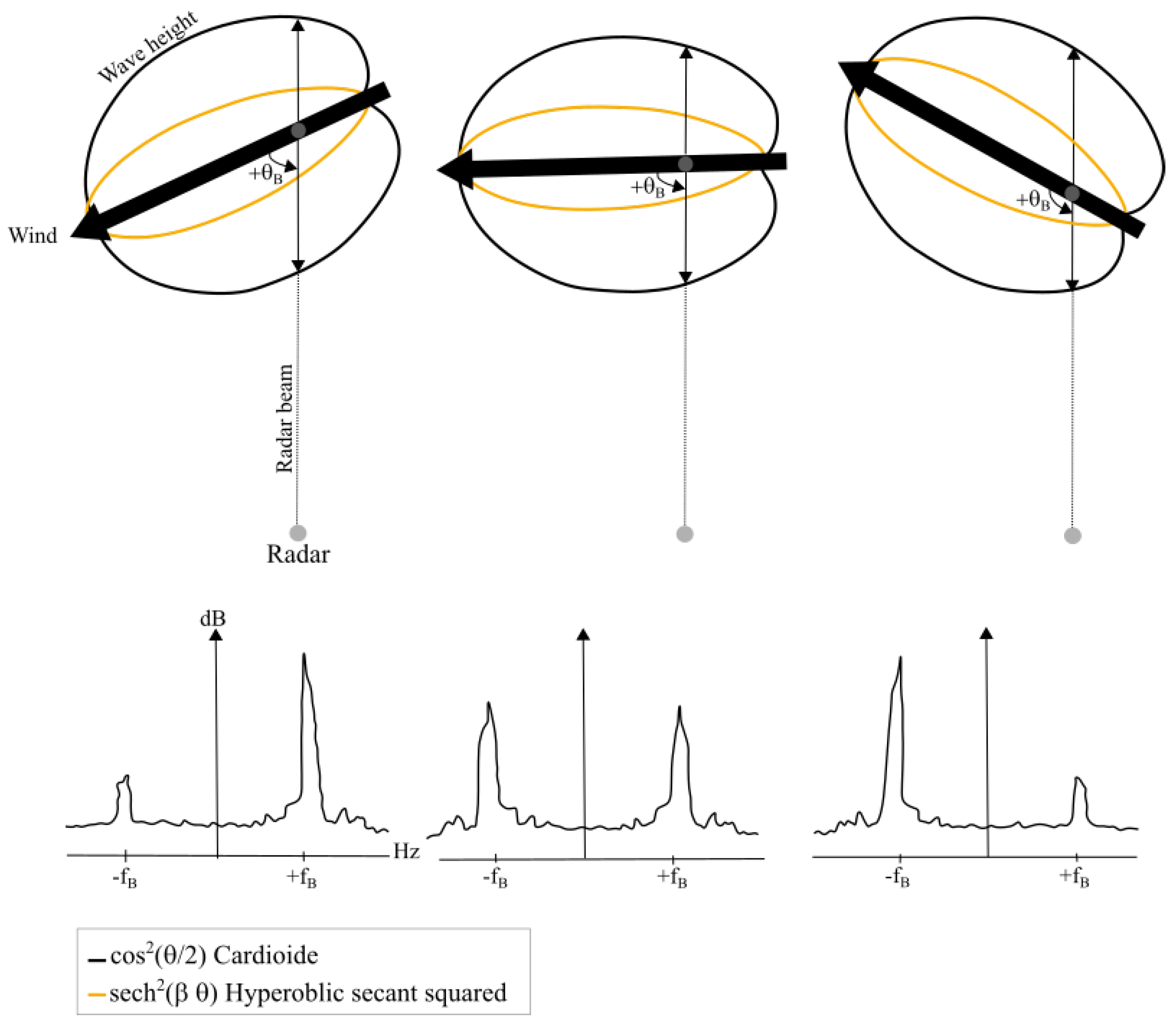
where is the angle relative to the wind direction and is the directional spreading parameter. In the literature, a number of directional distributions have been proposed, in particular, the cardioïd distribution which is often used (Figure 2, black line). However, we choose the squared hyperbolic secant function (see Figure 2, orange line) because it has been demonstrated to provide the most realistic upwind to downwind ratio conditions for ocean wavelengths ranging from 5 to 20 m [11].
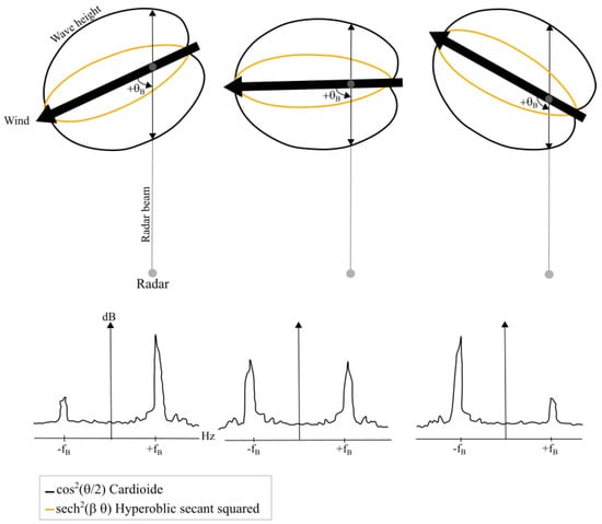
Figure 2.
The distributions of surface wave energy relative to the wind direction angle are illustrated for scenarios with the wind blowing towards (left), at a right angle (middle), and away from (right) the radar look direction. The backscatter spectra below illustrate the relative heights of the approaching () and receding () Bragg peaks for each corresponding case. This figure is adapated from Fernandez et al. (1997) [3].
The directional spreading parameter is expressed as [15]
where is the Bragg wavenumber and is the peak wavenumber.
The ratio of energy between approaching and receding Bragg waves is
where is beam direction of the radar and is the wind direction.
For each radar grid point, solving for yields two possible solutions [11]
which are, respectively, to the left and to the right of the radar beam direction. Traditionally, to resolve this directional ambiguity, estimates from a second radar site that observes the same ocean grid point from a different angle are used (e.g., [3]). However, this limits the area where the wind direction can be estimated without ambiguity to the overlap of the areas observed by both radars, which is generally smaller than the areas observed by each radar.
Huang et al. (2004) [4] proposed an algorithm to remove the ambiguity for a single radar site. Which direction to choose (left or right) is determined by minimizing the sum of the absolute differences among all possible wind directions derived from three different radar beams (see Equation (10) in [4]). Their algorithm relies on the assumption that wind directions vary slowly across the radar domain. We make the same assumption, but use a different method to remove the wind direction ambiguities with a single HF radar. For each grid point, we select all grid points with radar beam directions within of the reference beam direction, and with ranges within km of the reference range (Figure 3), and estimate and for all these grid points. The idea is that for each grid point either or will yield the correct wind direction, which should be similar for all grid points, while the other solution will yield an incorrect wind direction, which should differ among all grid points (see Figure 3). Hence, the true wind direction representative of the selected area, , is given by the modal direction of the histogram of all possible directions (merging and together, see Figure 4). Finally, the wind direction at the reference grid point is the one that minimizes the absolute difference with .
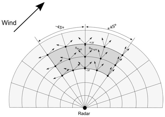
Figure 3.
Schematic to remove the wind directional ambiguity using a single HF radar. The gray area is used to obtain the histogram of all possible wind directions.
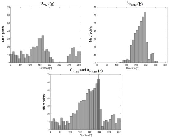
Figure 4.
Histograms of (a) the left solutions, (b) the right solutions and (c) both solutions (left and right). The modal direction is indicated by the vertical line in (c).
2.2. Wind Speed Estimation by a Single HF Radar
We propose to estimate wind speed with a method based on radar-measured wind-driven currents and wind directions estimated as above, in which an ANN is employed to determine a statistical relationship between wind-driven currents and wind speed. The ANN is a statistical learning algorithm capable of performing rapid, non-linear calculations and processing complex information. Usually, ANNs are employed to estimate unknown functions dependent on multiple inputs. The architecture of an ANN comprises interconnected nodes, or neurons, each representing a specific transfer function. Different weights are assigned to the connections between nodes, serving as memory for learned patterns. The learning process of an ANN involves adjusting these weights based on a provided training data set.
We decompose the radial surface current () measured by the HF radar into three components
where is the tidal current, is the time-averaged current, is the residual current, r and are range and bearing of HF radar, and t is time. To obtain residual currents, tidal and mean currents are removed from the radar-measured surface currents (see Equation (6)). Tidal currents are estimated using the Matlab T-Tide harmonic analysis toolbox [16]. The residual currents include wind-driven currents plus time-varying geostrophic currents that cannot be estimated from HF radar measurements. The wind-driven currents include currents driven by the wind stress and Stokes drift induced by the surface waves [17].
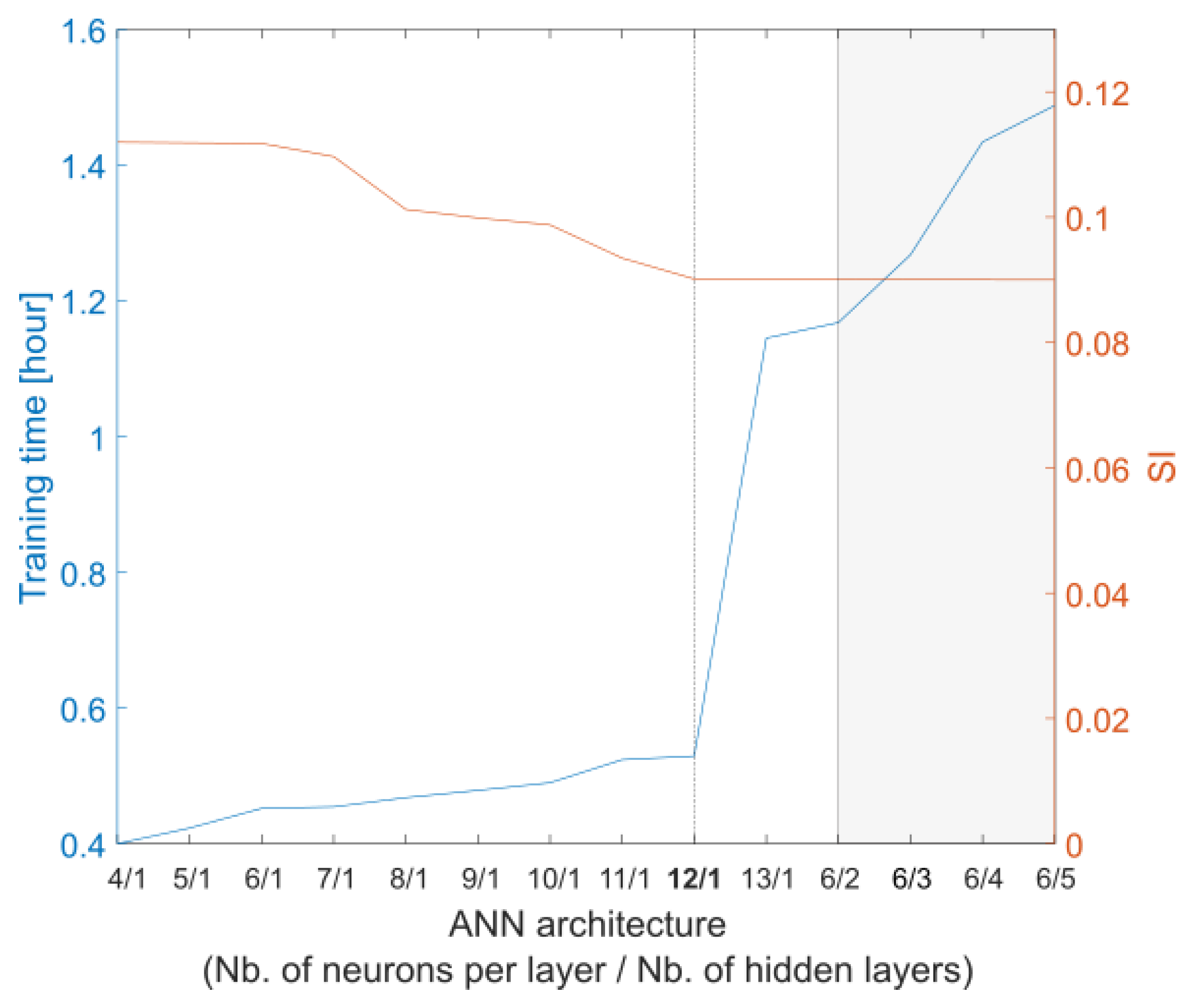
The relationship between wind-driven current speed and wind speed is complex and cannot be precisely expressed through an analytical expression. ANNs serve as a network structure specifically designed to handle the complex and unknown relationships between dependent parameters. The back-propagation (BP) neural network stands as the most commonly utilized type of ANN, featuring an input layer, hidden layer(s), and an output layer. In BP, the network error gradient with respect to the weights is computed, and subsequent weight updates are performed in the opposite direction of the gradient. In the literature, it has been demonstrated that a three-layer BP network, with a sigmoid transfer function, has the capability to approximate nonlinear equations. To select the optimal architecture, it is necessary to explore different combinations, identifying the one that produces predictions within a specified tolerance. The network utilizes error BP training with a Levenberg–Marquardt algorithm and is implemented using MATLAB’s Neural Network Toolbox. The ANN takes de-tided radial HF radar currents and wind directions as inputs, with the output being the wind speed. The performance of a neural network relies on its architecture. Selecting the optimal architecture is not governed by universal rules; rather, this process may entail a trade-off between computational time and performance (Figure 5), prompting the user to prioritize one based on their specific requirements. Here, the ANN structure consists of three layers, with four neurons in the input layer, twelve neurons in the hidden layer, and three neurons in the output layer (Figure 6).
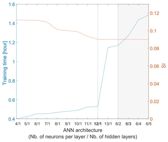
Figure 5.
Training time and SI (relative to buoy PMZA-Riki observations) for different ANN architectures.

Figure 6.
ANN structure used for wind field estimations with a single HF radar.
Training for this ANN configuration is carried out using wind data from the buoy PMZA-Riki, and current data from the WERA W2 and the CODAR C1 for the summer 2013. For the winter 2016–2017, the wind data from the meteorological station in the Bic Channel and the current data from the WERA W1 and the CODAR C1 have been used. Separate ANNs are trained for WERA and CODAR radars due to their different radio frequencies. For each ANN, the input parameters are exclusively sourced from a single radar. In this work, we chose to allocate 70% of the data randomly as the training dataset, while the remaining data was split into a validation set (15%) and a test set (15%). Training is based on the differences between the network’s output and the observed wind speed (loss function). Training is considered optimal when the loss function reaches a local minimum. The training dataset serves to calibrate the internal weights of the ANN, whereas the validation dataset is used during the iterative training process to determine the point of best ANN prediction while avoiding over-fitting. The test dataset serves the distinct purpose of independently assessing the skill of the final ANN model.
2.3. Statistical Analysis of Data
Two metrics have been used to compare the results of our methods with observations. For the wind field, we use the complex correlation coefficient [18]
where is the observed wind speed (in complex form ), is the wind speed estimated from the radar, and the asterisk indicates the complex conjugate. The complex correlation can be written as , where represents the average angle between and . For the wind direction and speed, we use the median-product correlation coefficient defined by Shevlyakov et al. [19] as
where and (see [17] for a detailed description and justification of this choice).
Confidence intervals for the correlation coefficients are determined through the bootstrap method, by generating 1500 bootstrap samples from the original linear regression residuals, as detailed in [20].
To assess the accuracy of HF radar wind speed estimations in comparison to previous studies, we employ the scatter index, as defined by byWyatt (2022) [13] as
where is the maximum of the wind speed and is the root mean square wind speed differences.
3. Study Area and Data
3.1. Study Area
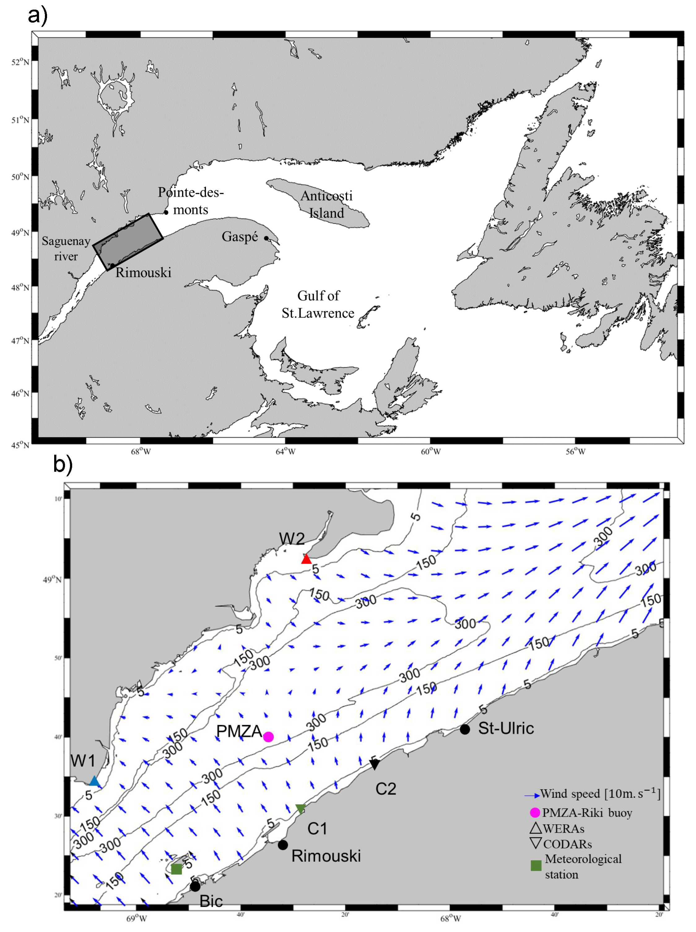
Our study area is the Lower Saint Lawrence Estuary (LSLE) in Québec, Canada (see Figure 7). The LSLE stretches between 20 and 50 km in width, extending from the mouth of the Saguenay River to Pointe-des-Monts [21]. The LSLE is a vertically and laterally stratified estuary, where baroclinic coastal currents, density fronts and eddies can form due to buoyancy fluxes and baroclinic instabilities [22]. Currents in the LSLE are also driven by winds [23], river outflows [24], and tides [25]. The tidal pattern in this region is primarily semidiurnal, with tidal amplitudes increasing from downstream to upstream [26]. The prevailing waves in the LSLE are commonly generated by local winds that mainly blow from the southwest. These winds reach their peak intensity during the winter season and are channeled along the estuary’s longitudinal axis by the coastal mountains on both shores [22].
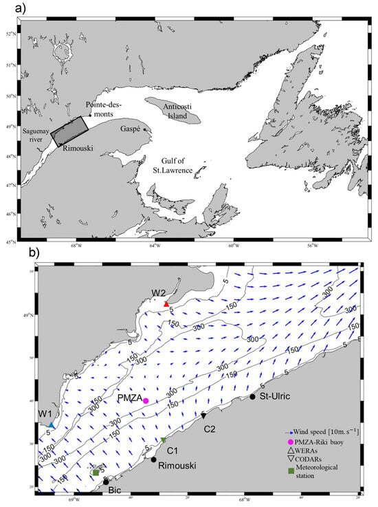
Figure 7.
(a) Map of the Gulf and (b) the lower Estuary of Saint Lawrence. The black-outlined rectangle in (a) delimits the study area in the lower Saint Lawrence Estuary. The instrument locations are indicated, and the wind field predicted by a numerical model, for the 1 January 2017 at 23h00, is shown by the blue arrows. The black lines indicate isobaths.
While surface waves are often constrained by fetch limitations, wave heights can frequently attain 1 m and occasionally surpass 3 m [27]. Between October 2016 and April 2017 (winter 2016/17), the study area experienced primarily moderate winds from various directions (see Figure 3a in [17]). During winter storms, wind speeds could surpass 20 m/s, creating favorable conditions for the development of storm waves. From May to October 2013 (summer 2013), prevailing winds predominantly blew from the southwesterly and northeasterly directions (see Figure 3b in [17]).
3.2. Data
3.2.1. HF Radars
Since November 2012, four high-frequency (HF) radars have been deployed and operational in the LSLE, measuring hourly surface currents. This study utilizes radar measurements obtained during the summer of 2013 and winter 2016–2017. Two Coastal Ocean Dynamics Applications Radars (CODARs) were positioned on the south shore of the LSLE (C1: N, W, with a frequency of MHz; and C2: N, W, with a frequency of MHz). On the north shore, two Wellen Radars (WERA) were deployed (W1: N, W; and W2: N, W), both operating at a frequency of MHz. Detailed radar system parameters for this experiment are provided in Section 2.b of [17]. To minimize measurement noise, we implemented the majority of the quality control tests outlined in QARTOD [28] (see [17] for a detailed description). This included the application of a signal-to-noise ratio (SNR) threshold, as detailed in Section 4.
To determine the direction of the backscattered sea echoes, WERAs and CODARs use different techniques: beam forming and direction finding, respectively. With the direction finding technique, we use the ratio of the SNR of each Bragg peak to obtain the ratio of the Bragg peaks power R (see Figure 1). The SNR of the Bragg peaks and the radial currents are obtained from the radial metric files, which were processed using the toolbox of B. Emery [29]. With the beam forming technique, the Bragg peak powers were obtained directly from the beam-formed spectra, which are used to compute the radial currents, and were processed with the package of Gurgel et al., 1999 [30]. Both WERAs and CODARs data were hourly averaged.
3.2.2. Meteorological and Model Data
During summer 2013, an oceanographic buoy (PMZA-Riki, N, W, operated by Institut Maurice-Lamontagne; Figure 7) was moored in the field of view of the radars and measured wind direction and speed at 10 m height every 15 mn. During winter 2016–2017, there was a meteorological station located on Île Bicquette (N, W) that measured wind direction and speed at 10 m height every half hour.
In addition, hourly wind speeds were acquired from a regional configuration of the High Regional Deterministic Prediction System (HRDPS) atmospheric model, centered over the St. Lawrence Estuary, with a horizontal resolution of km. This model is operated by Environment and Climate Change Canada for weather prediction [31].
4. Results
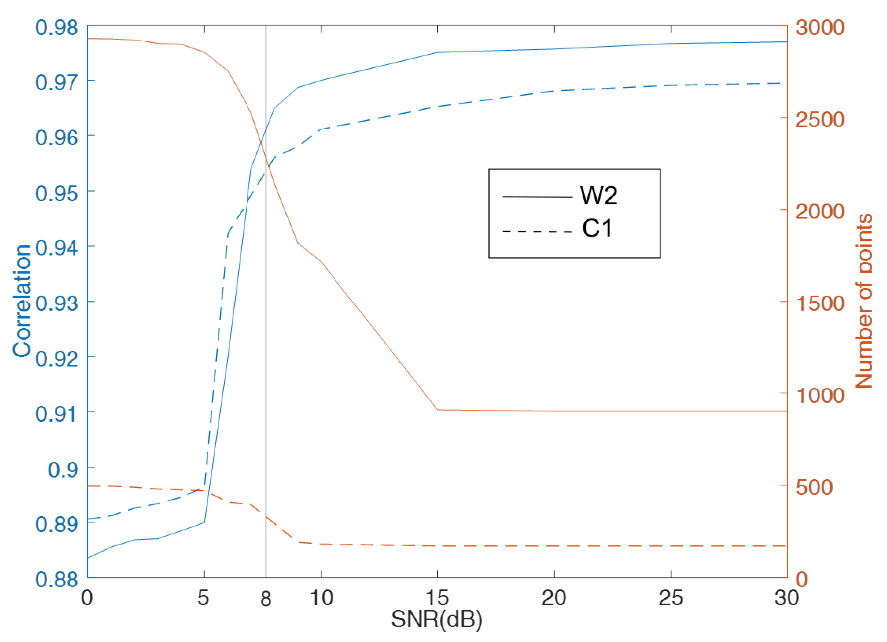
One of the most important quality control parameters is the SNR of the Bragg peaks. Figure 8 shows the correlation coefficient between the observed wind direction and that estimated from the radar data as a function of the SNR threshold value. Correlation coefficients increase from at to at for all HF radars, but the number of observations sharply decrease for . Thus, we choose an threshold of 8 dB as a compromise between data quality and quantity.
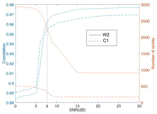
Figure 8.
Correlation between radar-estimated and in situ wind direction (blue lines) and number of data points (red lines) as a function of SNR threshold values, for W2 WERA (solid lines) and C1 CODAR (dashed lines).
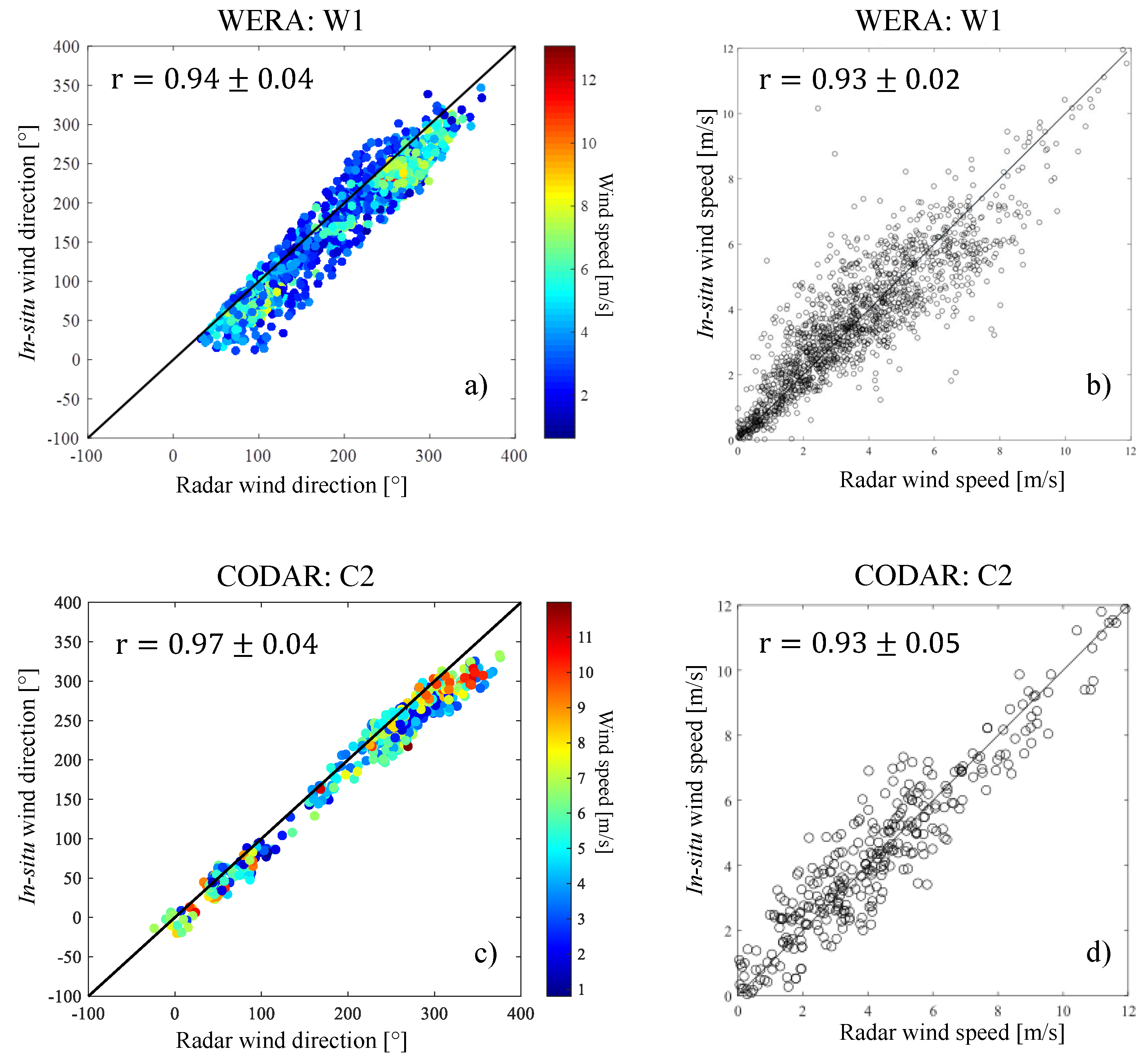
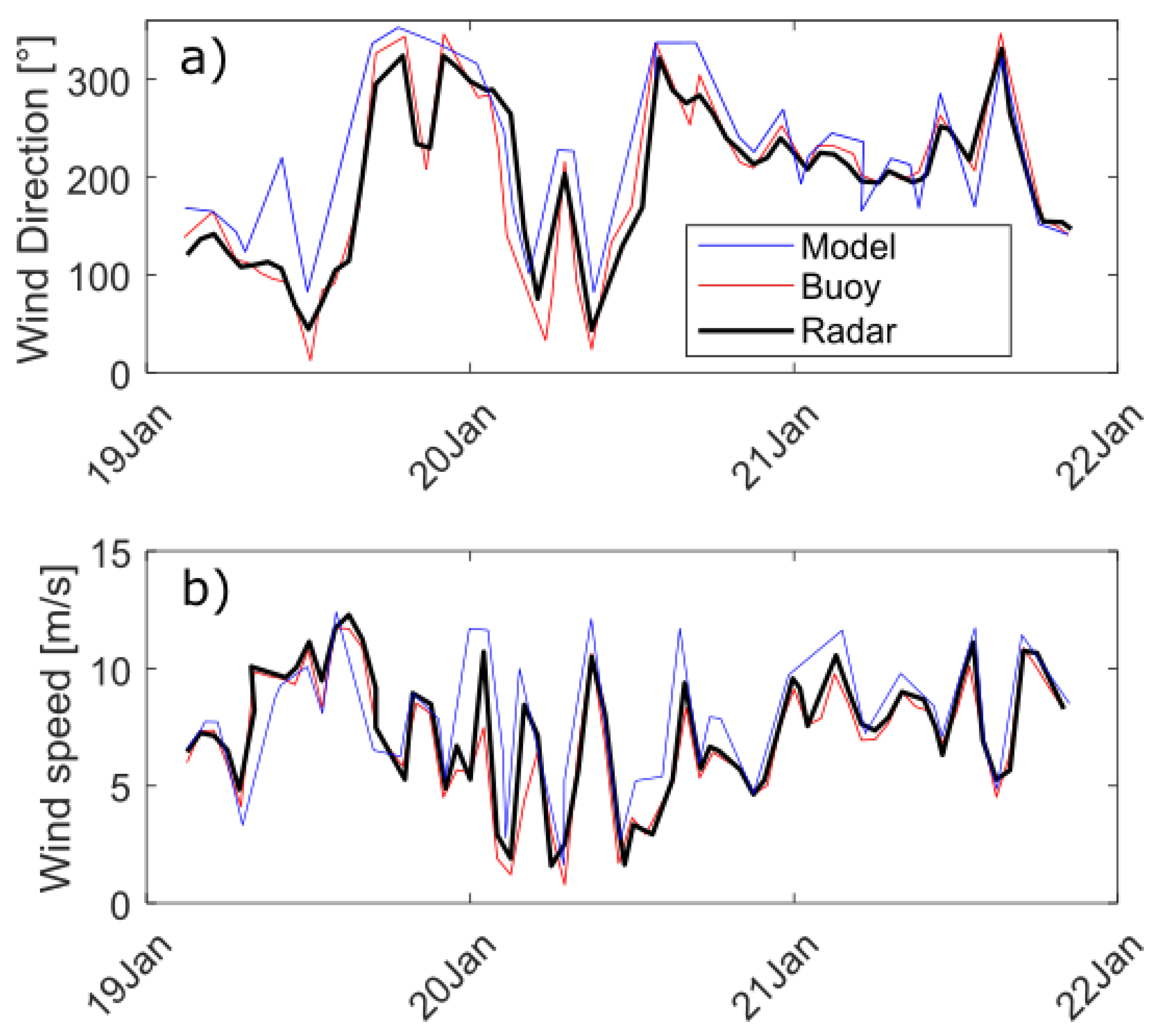
Figure 9 shows scatterplots of wind directions and speeds measured at PMZA-Riki buoy versus estimated from the closest radar data during summer 2013. Correlation coefficients are above . There is less scatter but also less data for the CODAR than for the WERA radar. Wind directions are slightly better correlated and have less scatter than wind speeds. As a result, wind speed time series estimated from radar data are noisier than in situ observations, but the low-frequency temporal variability is well resolved (Figure 10). Columns 2–5 of Table 1 summarize the statistical comparisons between wind field estimated and measured for all HF radar–in situ instruments pairs. For wind direction, the highest correlations (0.90–0.96) are obtained during the summer 2013. For wind speed, the average correlation coefficient is for all types of HF radars.
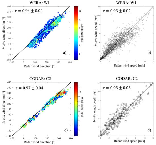
Figure 9.
Scatterplots of (a,c) wind direction and (b,d) wind speed estimated from (a,b) W1 WERA and (c,d) C2 CODAR versus in situ measurements in summer 2013.
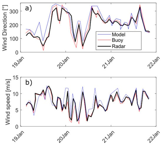
Figure 10.
Time series of (a) wind direction and (b) wind speed in winter 2016–2017 from in situ observations (red), numerical model HRDPS (blue) and W2 WERA (black).

Table 1.
Statistical metrics for the comparisons between HFR and in situ wind direction (first lines) and speed (second lines) for the summer 2013 and for the winter 2016–2017. For the radars that are used for training the ANNs, metrics are computed on the test datasets.
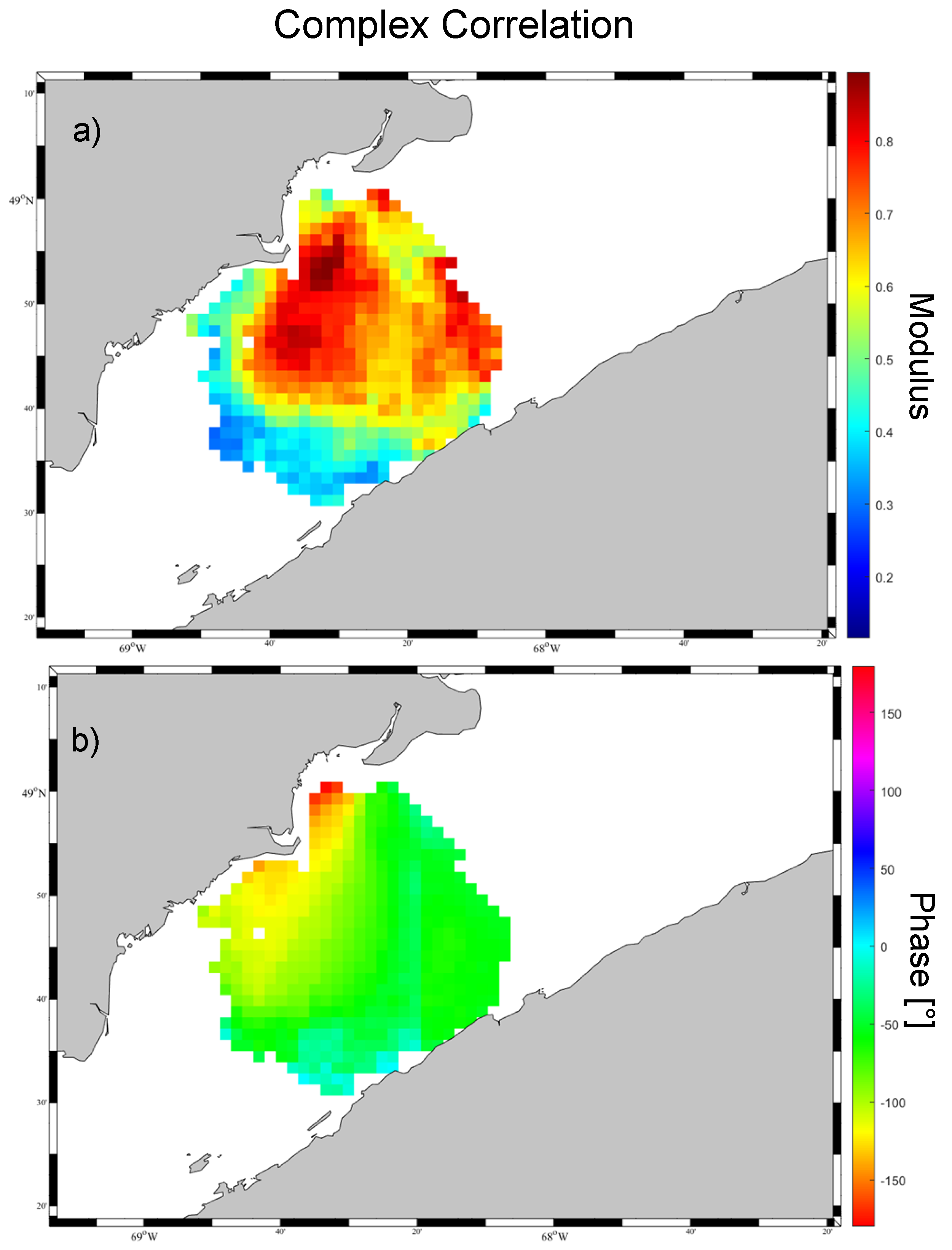
Comparisons with in situ observations are only available at specific locations. To characterize the spatial robustness of wind estimations from HF radars, we computed the complex correlation coefficients between wind vectors estimated from W2 WERA radar and simulated by the atmospheric model (Figure 11). In the region close to the radar, the modulus is higher than 0.7. However, the phase is non-zero over most of the region, because the radar data show greater spatial variability than the model (e.g., Figure 12).

Figure 11.
Spatial distribution of (a) modulus and (b) phase of complex correlation coefficients, R, between wind velocities estimated from W2 WERA and simulated by HRDPS for the winter 2016–2017.
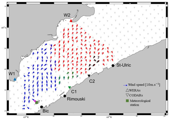
Figure 12.
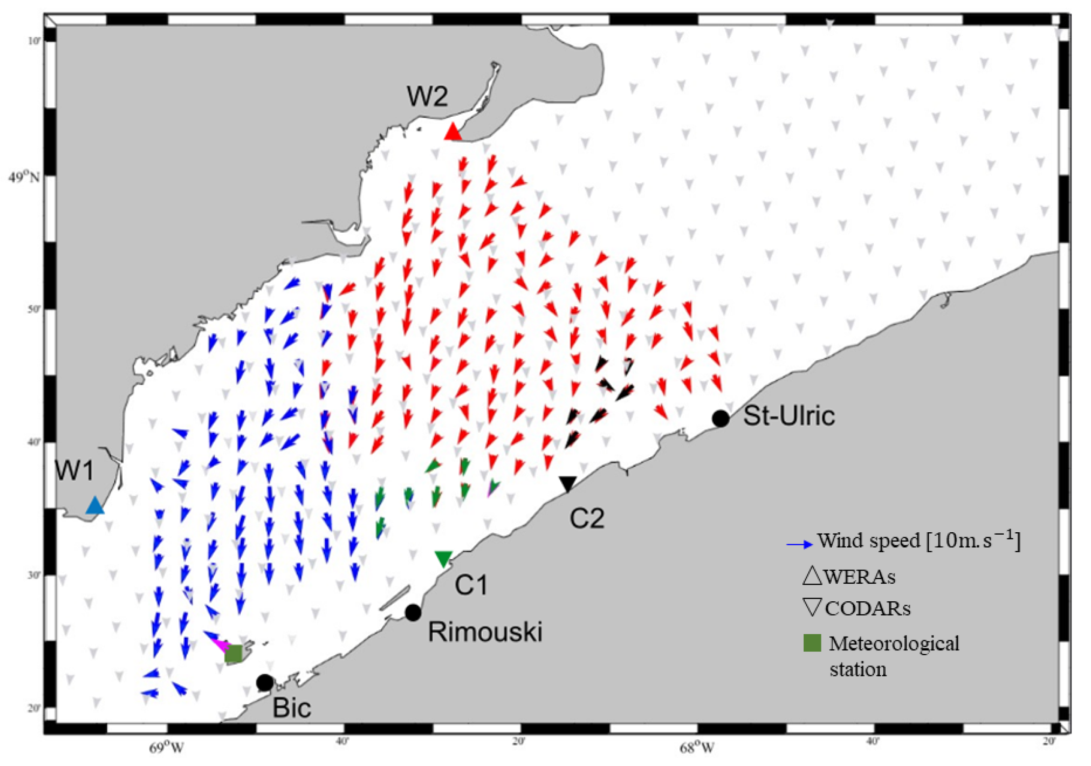
Winds estimated from W1 (blue arrows), W2 (red arrows), C1 (green arrows), C2 (black arrows), measured at Bic station (magenta arrow), and simulated by HRDPS model (gray arrows) at 11h00, 27 January 2017.
5. Discussion
To determine the wind direction from data acquired by a single HF radar is challenging due to inherent direction ambiguities. Huang et al. (2004) [4] proposed an algorithm to resolve the ambiguity assuming that wind directions vary slowly over the observational domain. Based on the same assumption, we propose a different method which yields improved results (an average increase in correlation coefficients of approximately 14%, not shown).
Several methods have been proposed in the literature to derive wind speed from HF radar measurements, which always required data from at least two overlapping radars. Here, we propose a novel approach for estimating wind speed from the first-order radar spectral peaks, yielding the same spatial coverage as for radial currents. Table 2 compares our results with those of previous studies using two metrics: the correlation coefficient and . The first method, as outlined in Table 2, is the inverse wind–wave modeling approach by Dexter and Theodoridis (1982) [6], which relies on the second-order spectrum. However, this method becomes less reliable in the presence of swell, particularly in conditions of light winds [13]. Other methods exclusively utilize the first-order spectrum and encompass partial least squares (PLS) [10], ANN [11,12,32], and physical models for first-order amplitudes [33,34]. Furthermore, Zeng et al. (2016) [32] utilized different metocean parameters, which include mean period, significant wave height and wind direction as inputs in their ANN approach. Some of the correlation coefficients for HF radar wind speed estimations that have been obtained in this study, as summarized in column 4 in Table 2, are higher than any reported values in the literature. Furthermore, some of the of the HF radar wind speed estimations surpass any reported in the literature to date (see column 5 in Table 2).

Table 2.
Comparisons of published methods for estimating wind speed from HF radars. * We read the limits on Figure 7 in [12]. This table is adapted from Table 1 in Wyatt (2022) [13].
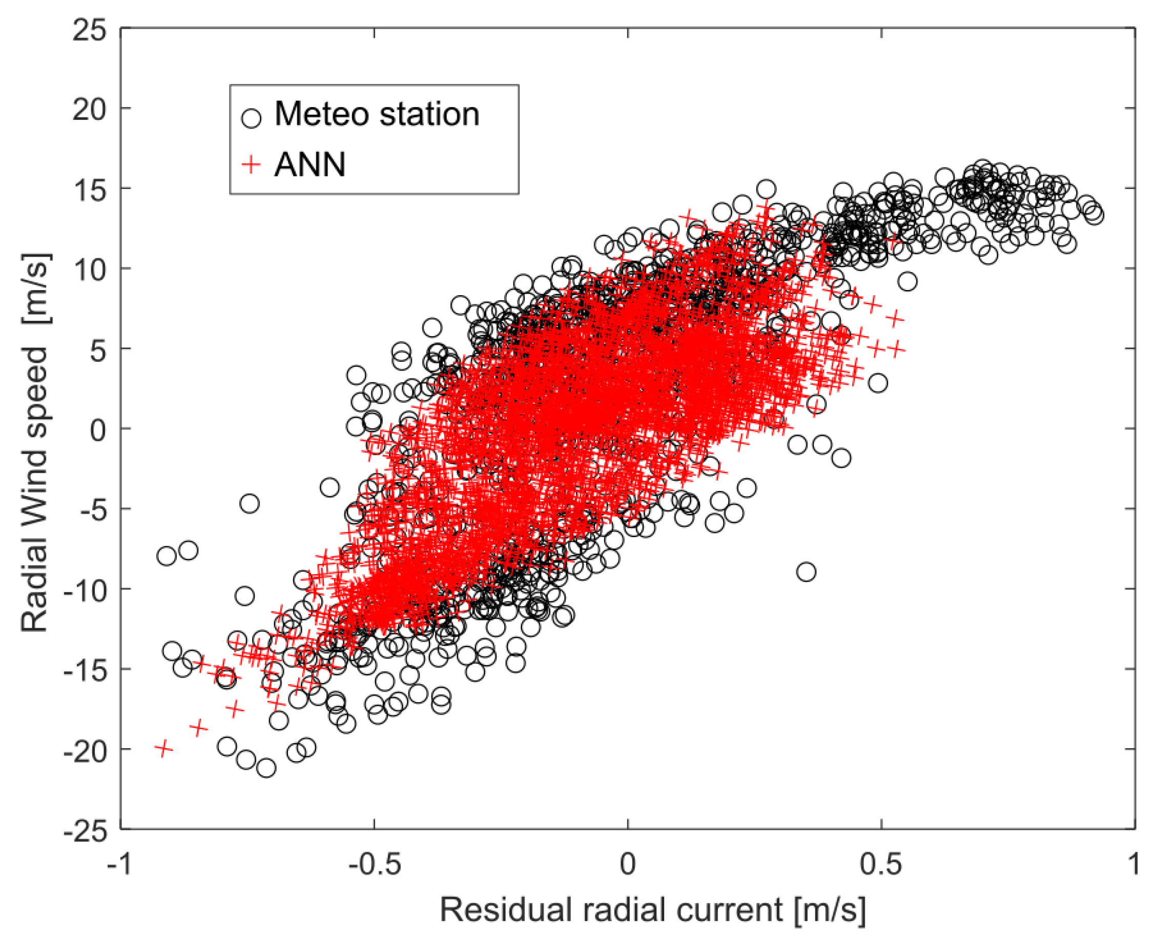
Our method to estimate wind speed is similar to that used by Wen et al. (2020) [12] but is based on radial currents instead of vector currents as input to the ANN, so it can be applied to a single HF radar. The method relies on wind-induced currents dominating the residual currents measured by the HF radar (defined in Equation (6)), as shown in Figure 13 (see also Figure 5b in [12]). In regions where wind-induced currents are not dominant, the methodology proposed here may encounter limitations. To address this issue, multi-frequency radars should be used to measure currents at different effective depths, yielding measurements of the currents vertical shear, which should be used as the input for the neural network in addition to the wind direction. This should enhance the model’s adaptability to diverse environments, since near-surface current shear is mostly wind-induced [35].

Figure 13.
Wind speed projected in radar direction, shown in black for the meteorologic station and in red for the ANN, versus residual radial current from W2 in winter 2016–2017.
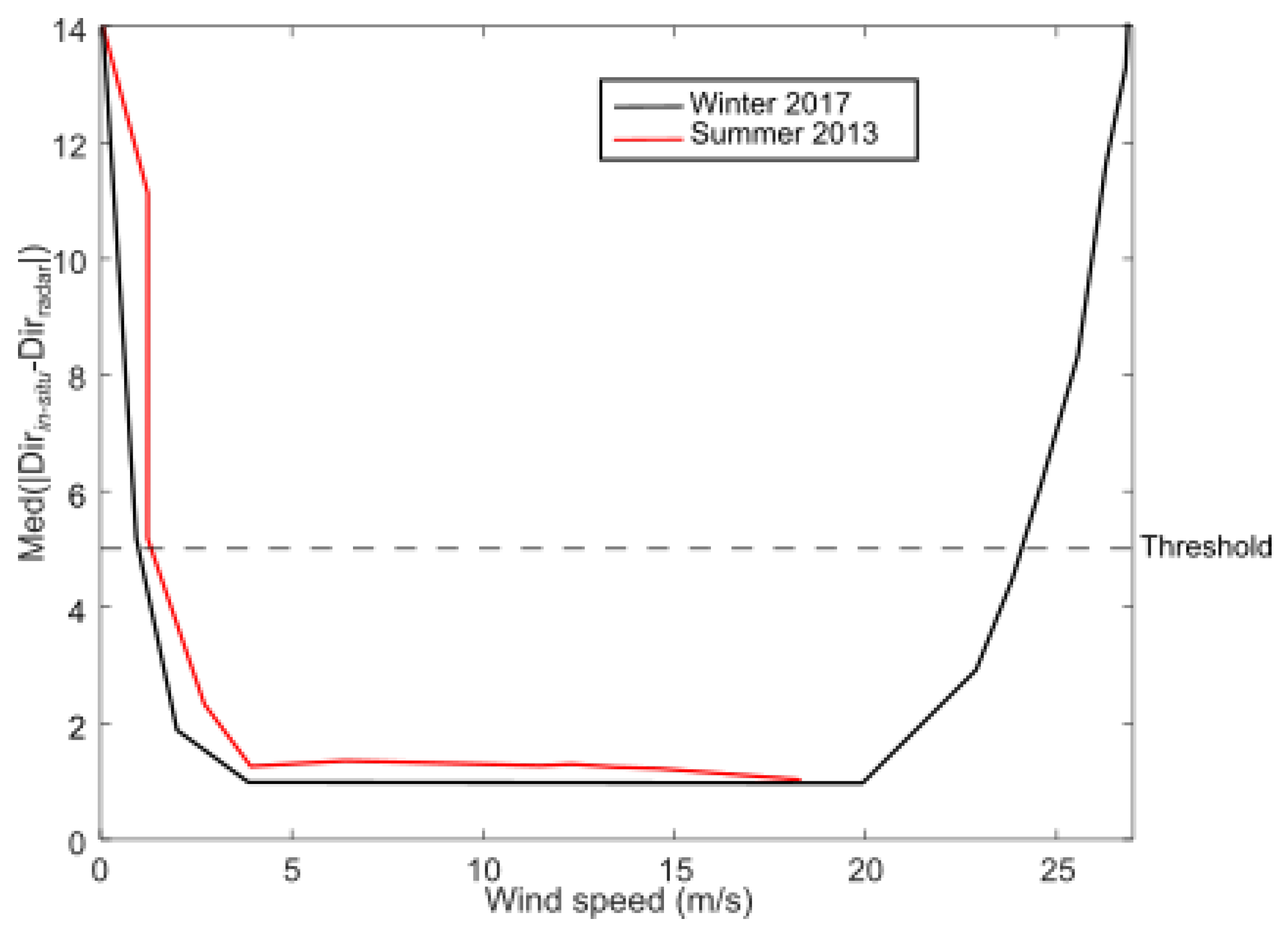
The wind direction and speed estimated with HF radars rely on the relationship between wind and surface waves and currents. However, a consequence of utilizing the first-order peaks of the radar’s Doppler spectrum is the limit of the relationship to a single frequency in the ocean wave spectrum, corresponding to the radar’s frequency-dependent Bragg resonant ocean waves. This limitation confines the range of wind speeds that the specific Bragg frequency can effectively respond to. In previous studies, comparisons between wind inversion methods for light winds (see Figures 9, 11 and 13 in [11] or Figures 3 and 6 in [32]) revealed low limitations attributed to the absence of Bragg waves under such conditions, rendering radar observations ineffective [11]. However, our results, similar to Figure 7b in Wen et al. (2020) [12], do not exhibit the same limitation. A possible explanation is that when low wind speed periods are sufficiently short, such as the example shown in Figure 10, Bragg waves do not have time to be completely damped before being reinforced again by the wind, and therefore, HF radars are still measuring surface currents during these low-wind conditions, enabling the ANN to infer the low wind speeds. However, to identify the range of wind speed for which our method yields accurate wind directions, we computed the average absolute value of differences between in situ and radar wind directions versus wind speed (with 1m/s bins, see Figure 14). Our method yields an average accuracy better than 5 degrees for wind speeds ranging from 2 m/s to 24 m/s.
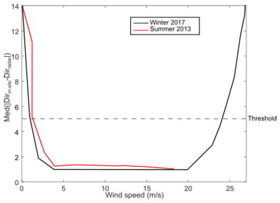
Figure 14.
Median absolute value of differences between in situ and radar wind directions versus wind speed in winter 2017 (black line) and summer 2013 (red line). Dashed line indicates a threshold value of 5 degrees.
6. Conclusions
The utilization of HF radars for wind mapping offers the advantage of providing data across a broad area with high spatial and temporal resolution. By using the first-order spectral peaks from a single HF radar, our method provides identical spatial coverage as observed for radial surface currents. The method uses an ANN to establish the relationship between residual radial currents and wind direction as inputs, and wind speed as the output. After training, the precision and adaptability of the ANN are verified over two distinct periods: summer 2013 and winter 2016–2017, utilizing data from four different radars. The correlation coefficients between radar-estimated and in situ wind directions range from to for the WERAs and from to for the CODARs. Similarly, the correlation coefficients between radar-estimated and in situ wind speed range from to for the WERAs and from to for the CODARs.
In exploring the adaptability of this trained ANN to different locations or radar frequencies, it is essential to acknowledge inherent limitations. The applicability of the ANN, as showcased in this study, is precisely tuned to the environmental conditions and radar frequencies employed during its training and validation. Therefore, applying this ANN to another radar of the same frequency but in a different environment, or another radar in the same environment but at a different frequency, should be approached with caution. As an example, we used the ANN trained by the C1 radar (12.5 MHz) and applied it to estimate wind speed using data from the W1 radar (16.15 MHz), yielding a decrease in correlation coefficient with observed wind speed of ∼0.1. Despite this limitation, the method’s interest lies in its capability to train the ANN using an in situ meteorological station for a limited period. Following the training phase, the ANN can be employed for subsequent HF radar operations. In the future, further validation will be necessary under various environmental conditions and radar frequencies.
Author Contributions
Writing—original draft, A.D.; Supervision, C.C. All authors have read and agreed to the published version of the manuscript.
Funding
We acknowledge the Fonds de recherche du Quéebec–Nature et technologies (FRQNT), the Marine Environmental, Observation, Prediction and Response Network (MEOPAR), Canada Economic Development for Quebec Regions, and Québec-Océan for their financial support. This research was supported by the Natural Sciences and Engineering Research Council of Canada (NSERC) under Grant No. RGPIN-2018-06585. We are grateful for their financial assistance, which made this study possible.
Data Availability Statement
The meteorological data used in this study are available on the Global Observatory of the St. Lawrence (OGSL) website. Additionally, the HF radar current data can also be accessed through the same platform.
Conflicts of Interest
The authors declare no conflict of interest.
References
- Long, A.; Trizna, D. Mapping of North Atlantic winds by HF radar sea backscatter interpretation. IEEE Trans. Antennas Propag. 1973, 21, 680–685. [Google Scholar] [CrossRef]
- Heron, M.; Rose, R. On the application of HF ocean radar to the observation of temporal and spatial changes in wind direction. IEEE J. Ocean. Eng. 1986, 11, 210–218. [Google Scholar] [CrossRef]
- Fernandez, D.M.; Graber, H.C.; Paduan, J.D.; Barrick, D.E. Mapping wind direction with HF radar. Oceanography 1997, 10, 93–95. [Google Scholar] [CrossRef]
- Huang, W.; Gill, E.; Wu, S.; Wen, B.; Yang, Z.; Hou, J. Measuring surface wind direction by monostatic HF ground-wave radar at the Eastern China Sea. IEEE J. Ocean. Eng. 2004, 29, 1032–1037. [Google Scholar] [CrossRef]
- Ahearn, J.L.; Curley, S.R.; Headrick, J.M.; Trizna, D. Tests of remote skywave measurement of ocean surface conditions. Proc. IEEE 1974, 62, 681–687. [Google Scholar] [CrossRef]
- Dexter, P.; Theodoridis, S. Surface wind speed extraction from HF sky wave radar Doppler spectra. Radio Sci. 1982, 17, 643–652. [Google Scholar] [CrossRef]
- Huang, W.; Wu, S.; Gill, E.; Wen, B.; Hou, J. HF radar wave and wind measurement over the Eastern China Sea. IEEE Trans. Geosci. Remote Sens. 2002, 40, 1950–1955. [Google Scholar] [CrossRef]
- Stewart, R.H.; Barnum, J.R. Radio measurements of oceanic winds at long ranges: An evaluation. Radio Sci. 1975, 10, 853–857. [Google Scholar] [CrossRef]
- Green, D.; Gill, E.; Huang, W. An inversion method for extraction of wind speed from high-frequency ground-wave radar oceanic backscatter. IEEE Trans. Geosci. Remote Sens. 2009, 47, 3338–3346. [Google Scholar] [CrossRef]
- Vesecky, J.F.; Drake, J.; Laws, K.; Ludwig, F.L.; Teague, C.C.; Paduan, J.D.; Meadows, L. Using multifrequency HF radar to estimate ocean wind fields. In Proceedings of the International Geoscience and Remote Sensing Symposium, Anchorage, AK, USA, 20–24 September 2004; Volume 7, p. 4769. [Google Scholar]
- Shen, W.; Gurgel, K.W.; Voulgaris, G.; Schlick, T.; Stammer, D. Wind-speed inversion from HF radar first-order backscatter signal. Ocean Dyn. 2012, 62, 105–121. [Google Scholar] [CrossRef]
- Wen, C.; Tian, Y.; Wen, B. Wind speed extraction based on high frequency radar retrieved wind-driven current. IEEE Geosci. Remote Sens. Lett. 2020, 18, 1555–1559. [Google Scholar] [CrossRef]
- Wyatt, L.R. Progress towards an HF radar wind speed measurement method using machine learning. Remote Sens. 2022, 14, 2098. [Google Scholar] [CrossRef]
- Donelan, M.A.; Hamilton, J.; Hui, W. Directional spectra of wind-generated ocean waves. Philos. Trans. R. Soc. Lond. Ser. A Math. Phys. Sci. 1985, 315, 509–562. [Google Scholar]
- Banner, M.L. Equilibrium spectra of wind waves. J. Phys. Oceanogr. 1990, 20, 966–984. [Google Scholar] [CrossRef]
- Pawlowicz, R.; Beardsley, B.; Lentz, S. Classical tidal harmonic analysis including error estimates in MATLAB using T_TIDE. Comput. Geosci. 2002, 28, 929–937. [Google Scholar] [CrossRef]
- Dussol, A.; Chavanne, C.; Gregorio, S.; Dumont, D. Experimental Confirmation of Stokes Drift Measurement by High-Frequency Radars. J. Atmos. Ocean. Technol. 2022, 39, 1541–1559. [Google Scholar] [CrossRef]
- Kundu, P.K. Ekman veering observed near the ocean bottom. J. Phys. Oceanogr. 1976, 6, 238–242. [Google Scholar] [CrossRef]
- Shevlyakov, G.; Smirnov, P.; Shin, V.I.; Kim, K. Asymptotically minimax bias estimation of the correlation coefficient for bivariate independent component distributions. J. Multivar. Anal. 2012, 111, 59–65. [Google Scholar] [CrossRef]
- Emery, W.J.; Thomson, R.E. Statistical Methods and Error Handling. In Data Analysis Methods in Physical Oceanography; Elsevier Science: Amsterdam, The Netherlands, 2001; Chapter 3; pp. 193–304. [Google Scholar] [CrossRef]
- El-Sabh, M.I. Physical oceanography of the St. Lawrence estuary. In Hydrodynamics of Estuaries, Volume II, Estuarine Case Studies; CRC Press: Boca Raton, FL, USA, 1988; pp. 61–78. [Google Scholar]
- Koutitonsky, V.; Bugden, G. The physical oceanography of the Gulf of St. Lawrence: A review with emphasis on the synoptic variability of the motion. In The Gulf of St. Lawrence: Small Ocean or Big Estuary? Proceedings of a Workshop/Symposium Held at the Maurice Lamontagne Institute, Mont-Joli, QC, Canada, 14–17 March 1989; Therriault, J.C., Ed.; Canadian Special Publication of Fisheries and Aquatic Sciences, 113; Fisheries and Oceans Canada: Ottawa, ON, Canada, 1991; pp. 57–90. [Google Scholar]
- Mertz, G.; Koutitonsky, V.; Gratton, Y.; El-Sabh, M. Wind-induced eddy motion in the lower St. Lawrence Estuary. Estuar. Coast. Shelf Sci. 1992, 34, 543–556. [Google Scholar] [CrossRef]
- Tee, K.T.; Lim, T.H. The freshwater pulse—A numerical model with application to the St. Lawrence Estuary. J. Mar. Res. 1987, 45, 871–909. [Google Scholar] [CrossRef]
- Forrester, W. Internal tides in St. Lawrence estuary. J. Mar. Res. 1974, 32. [Google Scholar]
- Drapeau, G. Dynamique sédimentaire des littoraux de l’estuaire du Saint-Laurent. Géographie Phys. Et Quat. 1992, 46, 233–242. [Google Scholar] [CrossRef]
- Didier, D.; Bernatchez, P.; Augereau, E.; Caulet, C.; Dumont, D.; Bismuth, E.; Cormier, L.; Floc’h, F.; Delacourt, C. LiDAR validation of a video-derived beachface topography on a tidal flat. Remote Sens. 2017, 9, 826. [Google Scholar] [CrossRef]
- Bushnell, M.; Worthington, H. Manual for Real-Time Quality Control of High Frequency Radar Surface Current Data: A Guide to Quality Control and Quality Assurance for High Frequency Radar Surface Current Observations; U.S. Department of Commerce, National Oceanic and Atmospheric Administration, National Ocean Service, Integrated Ocean Observing System: Silver Spring, MD, USA, 2016.
- Emery, B. HFR CS processing toolbox for MATLAB, v1.0. Zendo 2018. [Google Scholar] [CrossRef]
- Gurgel, K.W.; Essen, H.H.; Kingsley, S. High-frequency radars: Physical limitations and recent developments. Coast. Eng. 1999, 37, 201–218. [Google Scholar] [CrossRef]
- Smith, G.C.; Roy, F.; Brasnett, B. Evaluation of an operational ice–ocean analysis and forecasting system for the Gulf of St Lawrence. Q. J. R. Meteorol. Soc. 2013, 139, 419–433. [Google Scholar] [CrossRef]
- Zeng, Y.; Zhou, H.; Roarty, H.; Wen, B. Wind speed inversion in high frequency radar based on neural network. Int. J. Antennas Propag. 2016, 2016, 2706521. [Google Scholar] [CrossRef]
- Kirincich, A. Remote sensing of the surface wind field over the coastal ocean via direct calibration of HF radar backscatter power. J. Atmos. Ocean. Technol. 2016, 33, 1377–1392. [Google Scholar] [CrossRef]
- Emery, B.; Kirincich, A. HF radar observations of nearshore winds. In Ocean Remote Sensing Technologies—High-Frequency, Marine and GNSS-Based Radar; Institution of Engineering and Technology: London, UK, 2021; pp. 191–216. [Google Scholar]
- Teague, C. Multifrequency HF radar observations of currents and current shears. IEEE J. Ocean. Eng. 1986, 11, 258–269. [Google Scholar] [CrossRef]
Disclaimer/Publisher’s Note: The statements, opinions and data contained in all publications are solely those of the individual author(s) and contributor(s) and not of MDPI and/or the editor(s). MDPI and/or the editor(s) disclaim responsibility for any injury to people or property resulting from any ideas, methods, instructions or products referred to in the content. |
© 2024 by the authors. Licensee MDPI, Basel, Switzerland. This article is an open access article distributed under the terms and conditions of the Creative Commons Attribution (CC BY) license (https://creativecommons.org/licenses/by/4.0/).

