Abstract
The turfgrass industry supports golf courses, sports fields, and the landscaping and lawn care industries worldwide. Identifying the problem spots in turfgrass is crucial for targeted remediation for turfgrass treatment. There have been attempts to create vehicle- or drone-based scanners to predict turfgrass quality; however, these methods often have issues associated with high costs and/or a lack of accuracy due to using colour rather than grass height (R2 = 0.30 to 0.90). The new vehicle-mounted turfgrass scanner system developed in this study allows for faster data collection and a more accurate representation of turfgrass quality compared to currently available methods while being affordable and reliable. The Gryphon Turf Canopy Scanner (GTCS), a low-cost one-dimensional LiDAR array, was used to scan turfgrass and provide information about grass height, density, and homogeneity. Tests were carried out over three months in 2021, with ground-truthing taken during the same period. When utilizing non-linear regression, the system could predict the percent bare of a field (R2 = 0.47, root mean square error < 0.5 mm) with an increase in accuracy of 8% compared to the random forest metric. The potential environmental impact of this technology is vast, as a more targeted approach to remediation would reduce water, fertilizer, and herbicide usage.
Keywords:
turfgrass; sod; precision agriculture; LiDAR; non-linear regression; random forest; machine learning; RTK GPS 1. Introduction
Turfgrass is a USD 99 billion global industry [1]. In Canada alone, the turfgrass industry contributed CAD 149.7 million to the economy in 2021, an increase of 1.9% from 2020 [1]. This was accompanied by a 3.4% increase in total sod area [1]. However, two of the most detrimental issues for turfgrass farmers are poor knitting and fill in of the canopy, which lead to holes in sod rolls [2].
Turfgrass harvest requires the removal of the turf from the ground in rolls by a sod harvester. These sod rolls require the turfgrass to be sufficiently knitted together for the turfgrass to stay together during the cultivation and transportation processes [2]. The presence of holes in the turfgrass results in insufficient weaving of the sod and can result in tears and breaks in the rolls, rendering them unusable. Detecting these inconsistencies using remote sensing would provide a chance to remedy the sod before harvesting.
Remote sensing and precision agriculture techniques have become increasingly popular methods of detecting physiological and morphological traits in crops [3,4,5,6]. One remote sensing technology utilized heavily in recent years is LiDAR (light detection and ranging), due to its ability to accurately measure height [7]. LiDAR is a laser technology that calculates how far an object is away by measuring the amount of time the light from the LiDAR takes to reflect off the object and return to the receiver [8]. In precision agriculture, some examples of its usage include the estimation of biomass, land cover, forest canopy structure, and green area index, as well as plant identification [9,10,11,12]. However, little research has been conducted on the use of LiDAR as the primary source of data collection.
In studies utilizing terrestrial LiDAR, the LiDAR is often attached to a vehicle such that it can scan the area of interest unobstructed by the vehicle itself [4,12]. Wu et al. [5] successfully determined the structure of canola crops utilizing a ground-based LiDAR system called the Phenomobile. Furthermore, a relatively strong correlation (R2 = 0.61) was found in terrestrial LiDAR applications in measuring the biomass of tall fescue, a grass, utilizing a single 2-D LiDAR operating at 50 Hz compared to using NDVI (normalized difference vegetation index) measurements on their own (R2 = 0.56) [4]. Previous research utilizing drone-based LiDAR has primarily focused on crops with a much larger economic impact than sod, including area-wide mapping and forest canopy measurements, for which a ground-based vehicle would not be suitable [13,14].
Tow-behind sensors and robotics equipped with sensors are relatively new methods for measuring turfgrass quality. However, these sensors yield variable results and require continued validation to maintain accuracy because grass height is measured with horizontal beams that are broken at different heights [12,15,16]. Another challenge with the existing technology is that they cannot accurately and consistently differentiate between weeds and various grass species [12,16].
Using machine learning models to predict turfgrass quality with relatively high accuracy and spatial resolution has been promising [17,18]. However, machine learning models require high-level data processing technology, limiting their application at the farm level to obtain the necessary information accurately and affordably [17]. One solution allowing machine learning to move forward is to provide data that are easier to process yet still contain the necessary information to overcome the spatial variability in the turfgrass. In addition, the system should be able to determine variations in the structure of the turfgrass, which will give insights into the species present. Random forest is a machine learning method that has been successfully used for general-purpose classification that makes use of decision trees, where each tree gives a class prediction, and the class with the largest number of votes becomes the prediction [19]. Additionally, random forest models have been successful even when utilizing minimal input features [20].
Real-world terrestrial LiDAR applications almost always utilize a 2-D LiDAR, which has the beam rotate about a single fixed point. Although there has been some success with the implementation of these 2-D arrays, issues arise surrounding bare spot detection in sod due to complications related to viewing angle. Since the sensor is projecting the laser from a single point, bare spots can easily be obscured behind other blades of grass, giving an imprecise estimate of the size of the bare spot [21]. Issues surrounding the viewing angle for canopy cover detection related to 2-D LiDAR have not yet been discussed in detail. A 1-D LiDAR array would remove the viewing angle issue by scanning the turf at a 90-degree angle (Figure 1).
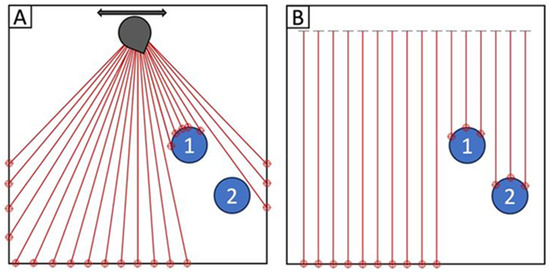
Figure 1.
Simplified illustration of (A) the viewing angle issue that typical 2-D LiDAR faces because of rotating from a fixed point and (B) a 1-D LiDAR array capable of capturing both objects.
The main goal of this study was to develop a 1-D LiDAR array that scans at a 90-degree angle, helping to overcome the issue of soil or bare spots being undetected behind blades of grass, as is the case with 2-D LiDAR and with current tow-behind units. Additionally, 1-D LiDAR can improve processing, allowing for faster data collection and utilization and expanding how the data can be interpreted later through machine learning with relatively low processing power. Compared to 2-D LiDAR, 1-D LiDAR is less expensive, making it more economically viable. A LiDAR array can also differentiate between different species of turfgrass and weed composition. The accuracy of a 1-D LiDAR array in predicting the bare percentage of sod field plots using random forest machine learning was determined.
2. Materials and Methods
Data collection occurred at the University of Guelph’s Turfgrass Institute (43°32′29.6″N 80°13′28.8″W) in Guelph, ON, Canada. Data were collected on a 22-metre by 34-metre field over three days in the summer/fall of 2021. The field was divided into 187 2 × 2 metre grid spaces, where ground truthing occurred (Figure 2). Each grid space was hand-truthed, utilizing half-metre point quadrats (Figure 3). Data collection required inspection of the field below each of the intersections of the quadrat. Four quadrats of 36 intersections were used on each 2 × 2-metre plot, resulting in 144 ground-truthed data points per plot. Each of the 144 points was marked as bare (having no grass) or grass (presence of grass) and was given a percent-bare value (the number of points considered bare divided by the total number of points) based on the quadrat point classification. The ground-truthed data from the point quadrats were used to train the models.
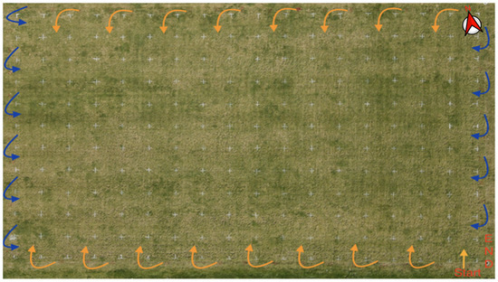
Figure 2.
The field set-up utilized for data collection and ground truthing at the University of Guelph Turfgrass Institute in Guelph, ON, Canada, during the summer/fall of 2021. The field was separated into 187 2 × 2-metre grid spaces. The orange arrows represent the movement of the Gryphon Turf Canopy Scanner (GTCS) vertically across the field in approximately a north-south pattern this was followed by movement horizontally across the field in approximately an east-west pattern.
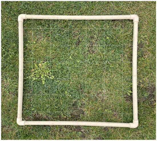
Figure 3.
Point quadrat used to ground truth the field at the Guelph Turfgrass Institute in Guelph, ON, Canada, in 2021. Ground truthing was used to identify bare versus healthy grass, where the points directly under the intersection of the wires were evaluated for a total of 36 points per point quadrat measurement.
The LiDAR array used for this research, referred to as the Gryphon Turf Canopy Scanner (GTCS), was assembled with 14 Garmin LiDAR Lite v3 sensors (Olathe, KS, USA), each attached to an Arduino (Figure 4). The LiDAR array was then attached to a Toro Triplex Mower (Bloomington, IN, USA), allowing use during regular turfgrass maintenance (Figure 4). Each LiDAR sensor was mounted perpendicular to the grass, with the corresponding Arduino next to each sensor recording the height from the ground in centimeters. The Arduino connected to the LiDAR recorded data onto a secure digital (SD) card, which automatically created a comma-separated values (CSV) file with two columns: height (cm) and time (ms). Time measurements began when the GTCS was turned on, with time stamps of every height recording taken.
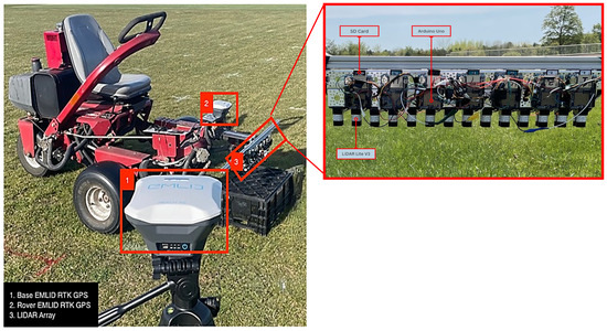
Figure 4.
The Gryphon Turf Canopy Scanner system (left), with a Rover EMLID RTK GPS and a 14 Garmin LiteV3 1-D LiDAR array connected individual Arduino Uno units and SD cards on a beam in front of a Toro Triplex Mower with Base EMLID RTK GPS in the foreground.
A real-time kinematic global position system (RTK GPS) was employed to track the location of the array as it moved around the field. The RTK GPS that was used was the EMLID RS (Budapest, Hungary), a low-cost solution capable of recording horizontal kinematic GPS data to 7 mm + 1 PPM. The RTK GPS was recorded at a frequency of 5 Hz. As each of the 14 LiDAR was physically offset from each other by 4 cm, 14 separate GPS files were created so that each LiDAR had its own set of unique coordinates. This process was completed utilizing the Geosphere package (Version 1.5-18) in R with WGS84 as its spatial reference.
Due to the frequency of data collection between the LiDAR and GPS datasets, the merging process required linear interpolation to create the positions of missing time stamps in the GPS data. A linear interpolation was assumed due to the direction and velocity of the GTCS between two consecutive GPS coordinates remaining approximately constant. Once the GPS and LiDAR data were combined, they were converted into a comma-separated values (CSV) file capable of being imported into QGIS. The 17 × 11 grid was recreated in QGIS utilizing WGS84 as its spatial reference. The CSV were then imported, and a function of QGIS called join attributes by location was used to bin the points within the 187 grid spaces. This joined layer was then exported back into R as a CSV to conduct a statistical analysis of the 187 bins.
A flowchart depicting data processing is highlighted in Figure 5. The LiDAR data were post-processed to calculate the mean and the standard deviation of the grass height within each bin. Z-score normalization of the data was used to preprocess the raw data before machine learning. Our machine learning and statistical models had only two input features (the mean and the standard deviation of the grass height), which is why the random forest and the nonlinear regression models were selected. These models allowed for the development of highly practical and simple-to-use models programmable within Microsoft Excel (Redmond, DC, USA). Our goal was to develop a farmer-focused sod management tool that matches the available skill sets and training readily available for practical applications within the sod-growing community.
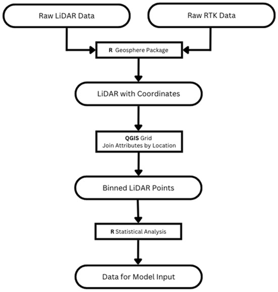
Figure 5.
The data workflow for measurements that were obtained by the Gryphon Turf Canopy Scanner system at the Guelph Turfgrass Institute in Guelph, ON, Canada, in 2021.
The models were trained using the GTCS and the ground-truthed data collected at different stages of the growing season. Machine learning algorithms were employed to determine what predictors, including the LiDAR measurement metrics, most accurately estimated turfgrass quality.
The datasets used were scans of the field recorded on 15 August, 24 September, and 13 October 2021. The two variables used as inputs for the algorithms were the Z-score normalized mean and normalized standard deviation of the grass height within each grid space. The response variable used was the bare percentage. The machine learning used was an out-of-the-bag (OOB)-style random forest carried out in XLSTAT by Lumivero (Denver, CO, USA) and did not require a validation set.
The performance of the machine learning models was evaluated using statistical error indices. If the values of these indices were reasonable, the best models were selected and presented. The trained/tested algorithms were used to process the LiDAR data and prepare a map of turfgrass quality as valuable and easy-to-use information to ensure the GTCS output is farmer-focused and easy to interpret.
The mdel’s performance error statistics were measured by comparing the actual results , predicted outcomes , and the mean of the actual values , where n is the number of samples.
- The root mean square error (RMSE) is computed as:
It is a widely used parameter to determine the performance of models [22].
- 2.
- The R-squared measures the discrepancy between the predicted and actual values. The equation is given by
- 3.
- The mean absolute percentage error (MAPE) indicates the absolute amount of error for predicted outcomes when compared to the actual values in a series [23].
The equation is given by
The nonlinear regression model (Equation (4)) for percent bare was developed using the Z-score normalized mean (M) and the Z-score normalized standard deviation (S) of the LiDAR-measured grass heights for each plot as the input.
The Microsoft Excel “Solver” function was used to optimize the empirical constants of the model using the generalized reduced gradient (GRG) nonlinear algorithm.
Although the model was only trained/tested on Kentucky Bluegrass, we have reason to believe the empirical constants in Equation (4) would be essentially similar for other commonly found grass species in urban landscapes. However, slight differences in the empirical constants can be expected across different grass species.
3. Results
Percent bare values were determined based on the point quadrat observations, either bare or grass. The observed percent bare values were correlated (R2 = 0.44) to the regression model’s (Equation (3)) predicted values (Figure 6) and had a lower correlation (R2 = 0.35) with the random forest prediction. A comparison of dates revealed that the 13 October 2021 date showed the most variation in bare percentage.
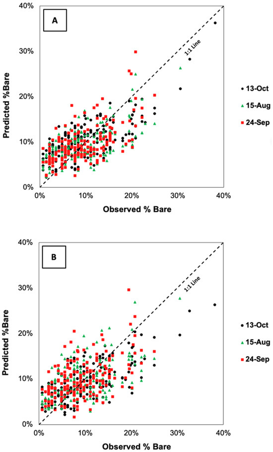
Figure 6.
Observed predicted percent bare plots for three scan dates (13 October, 15 August, and 24 September 2021) utilizing (A) a regression model and (B) a random forest model at the Guelph Turfgrass Institute in Guelph, ON, Canada.
Model performance for the random forest and the regression models was assessed by computing key performance metrics, including RMSE and R2 (Table 1). As shown, the R2 value for the regression model was 0.47 compared to 0.35 for the random forest model (Table 1).

Table 1.
Model performance statistics for the random forest and regression models on turf canopy heights taken at the Guelph Turfgrass Institute in Guelph, ON, Canada, in 2021.
Figure 7 presents the cumulative distributions of LiDAR-measured surface elevations (cm) for the bin with the highest bare percentage (B; bin 154) and the bin with the highest grass percentage (G; bin 169) for the 14 October 2021 scan. It is visible in the distributions that the average height of the grass is higher in bin 169 than in bin 154, and its curve is further right.
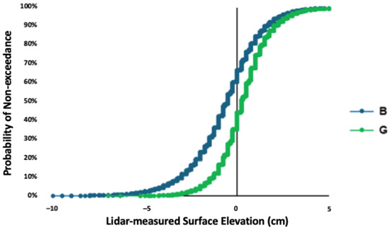
Figure 7.
A cumulative distribution function of two extreme bins (grid squares) with the highest percent grass (G; bin 169) and percent bare (B; bin 154) for the 13 October 2021 scan at the Guelph Turfgrass Institute in Guelph, ON, Canada.
Figure 8 presents a 3-D representation of the nonlinear regression model (Equation (3)), where the normalized mean grass height for the plot increases and the percent bare decreases. It also shows that as the normalized standard deviation of the grass height increases, the percent bare increases (Figure 8).
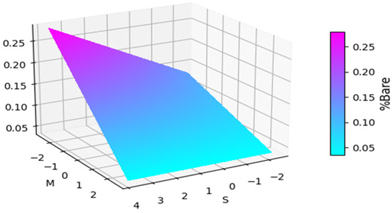
Figure 8.
A 3D representation of a non-linear regression model representing percent bare spots on plots at the Guelph Turfgrass Institute in Guelph, ON, in 2021. M and S represent the normalized mean and normalized standard deviation of the LiDAR-measured grass heights per plot, respectively.
A decision tree was created utilizing the mean and standard deviation of normalized heights of the field (Figure 9). The predictions (PRD) where the mean is less than −0.15 lead to a PRD of 21% and 14%, respectively. All means greater than −0.15 had a PRD 12%, with descending percentages as mean height increased. Additionally, the nodes where standard deviation was used as a branching point resulted in higher PRDs than those that used the mean.
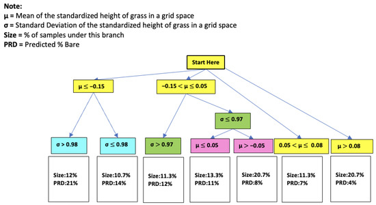
Figure 9.
Decision tree model structure based on the Guelph Turf Canopy Scanner (GTCS) measured heights at the Guelph Turfgrass Institute in Guelph, ON, Canada, in 2021.
Figure 10 depicts a graphical representation of the field, where comparisons can be made for a bare percentage between the ground-truth data (Figure 10A), the regression model (Figure 10B), and predicted values from the random forest model (Figure 10C). Scans for the maps were taken in October 2021, and three grid spaces were removed due to data outliers. The three maps identify a high percentage of bare grid spaces along the south side of the field (Figure 10). The random forest model was able to predict 70/184 (38%) with a percent bare value greater than 10% compared to the ground-truth and regression model data, which identified 78/187 (42%) and 90/184 (49%), respectively.
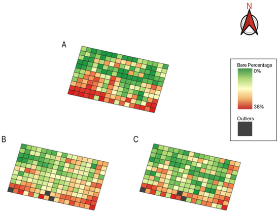
Figure 10.
Comparison of detection of turfgrass quality of 187 grid spaces for (A) ground-truth bare percent data, (B) the regression model’s bare percent data, and (C) the random forest model’s bare percent data. Data were collected at the Guelph Turfgrass Institute in Guelph, ON, Canada, in 2021.
4. Discussion
The presence of holes in sod rolls can result in tears and breaks, which render the rolls unusable [2]. High-throughput technologies, such as remote sensing, provide an opportunity to identify and remedy inconsistencies before harvest [24]. Table 2 highlights the use of LiDAR to measure phenotypic traits, including canopy height and biomass in several crops [25]. However, current LiDAR utility methods have been inaccurate for turfgrass due to a viewing angle issue [23]. This research sought to develop a method of using 1-D LiDAR technology to accurately measure canopy height for the turfgrass industry. Additionally, the improved processing power of 1-D LiDAR was explored for utilization in machine learning models for broader data applicability. Furthermore, the accuracy of a 1-D LiDAR array was determined for predicting the bare percentage of sod field plots using regression models and random forest machine learning and determining the effects of different normalization techniques on predictive modelling outcomes.
Table 2.
Summary of previously published remote-sensing-integrated biomass prediction models for various grass traits.
The experiment presented above highlights the utility of this technology for sod farms. As depicted in Figure 7, the standard deviation of the ‘grass’ bin had a steeper curve, indicating a smaller standard deviation for that bin. This is particularly important as sod farms consistently mow at a set height. Large deviations around this set height correspond to higher standard deviations, whereas lower standard deviations represent bin classes with few to no bare spots. Further, trends observed in Figure 9 showed that lower means and higher standard deviations resulted in higher predictions (PRD), which were apparent in the model output. The lower mean values represented bins where the grass had lower average heights compared to the mowing height, indicating potential bare spots. Increases in PRDs were expected, as a high prevalence of bare spots would increase the variability in the height of the bin.
LiDAR technology has been integrated in many industries, including the automotive, agriculture, consumer technology, and military industries [7,8,31]. However, the implementation of LiDAR technology largely encompasses 2-D LiDAR mounted on a single point. A key application of LiDAR in turfgrass is for bare spot detection; however, the angle at which the 2-D LiDAR measures distances results in the obscurement of bare spots due to blades of grass [12,16]. The viewing angle problem related to 2-D LiDAR has not been discussed in detail regarding detecting canopy cover and height. Therefore, the LiDAR array described in this research was designed to remove the viewing angle problem by scanning the turfgrass at a 90-degree angle with several LiDARs spaced close enough together to avoid missing bare spots, which would result in tears in the sod.
LiDAR applications in large-scale projects such as forest canopy scanning often use multiple-return LiDAR, which can overcome the barriers related to single-pass LiDAR by collecting multiple rounds of data. However, systems such as these are costly and usually have resolutions between returns unusable for a crop like sod [32,33]. Previous research exploring the integration of remote sensing and machine learning methods showed promise in grasses (R2 0.30 to 0.90); however, these methods have been largely applied to biomass predictions rather than height (Table 2). The data presented here highlight the value of using a 1-D LiDAR system for canopy height measurements in turfgrass with high accuracy (RMSE = 0.43 mm).
An additional advantage of utilizing a 1-D array with a set number of lasers comes with improved processing. Previous research has determined that another issue surrounding the use of high-quality LiDAR and other imaging techniques is the volume of data collected, potentially leading to processing issues [34,35]. This results in researchers deciding between image quality and processing capabilities for specific projects [36]. Furthermore, the 1-D LiDAR array presented in this paper offers the added benefit of being modular; thus, its size could be adjusted based on the project’s needs. This is important because of the variation in size of different sports fields and golf courses, among other applicable fields.
The benefit of incorporating a machine learning algorithm is its ability to use multiple indicators to determine turfgrass quality. Additionally, the ability of the random forest model to correctly identify the ‘good’ grid squares adds to the viability of this technology for real-world applications, as it would miss fewer harvestable spaces. Although the random forest model over-identified ‘good’ grid spaces, it essentially grouped them with ’medium’ grid spaces. This implies that the vast majority of misidentified grid spaces were still potentially harvestable. The improvement in this model, including the use of more complex methods capable of detecting small patterns in the turfgrass, may result in machine learning models that yield better results and require further testing.
The applicability of the GTCS extends beyond turfgrass, with implications in the detection and maintenance of pasture biomass in addition to golf courses, sports fields, and sod farms. Using a drivable bare spot detection system or an unmanned robotic system with a predetermined path plan will allow for the early detection of anomalies in sports fields and golf courses, preventing injuries to users and decreasing the costs associated with maintenance [37,38]. Along with identifying harvestability, there are potential ecological benefits to this technology by being able to locate good patches of sod that do not require as much intervention with either water or fertilizer for harvestability. A more targeted approach to fertilization and watering could be used to help reduce usage.
Identifying bare spots in turfgrass is crucial for targeted remediation before usage. This research presents a 1-D LiDAR approach that extends beyond the turfgrass industry by overcoming the viewing angle issue associated with 2-D LiDAR and incorporating improved data processing.
Author Contributions
Conceptualization, B.G. and E.M.L.; methodology, A.R., B.G. and E.M.L.; software, A.R.; validation, A.F. and A.R.; formal analysis, A.F. and A.R.; investigation, A.R.; resources, B.G. and E.M.L.; data curation, A.F. and A.R.; writing—original draft preparation, A.F. and A.R.; writing—review and editing, A.F., A.R., E.M.L. and B.G.; visualization, A.F., A.R. and B.G.; supervision, A.F., E.M.L. and B.G.; project administration, B.G. and E.M.L.; funding acquisition, B.G. and E.M.L. All authors have read and agreed to the published version of the manuscript.
Funding
This research was funded by the Natural Sciences and Engineering Research Council of Canada (NSERC) Alliance Grant #401643.
Data Availability Statement
The datasets presented in this article are not readily available because the data are part of an ongoing study. Requests to access the datasets should be directed to the corresponding author.
Acknowledgments
The authors would like to thank the Guelph Turfgrass Institute (GTI) staff for their help with the fieldwork portion of this research.
Conflicts of Interest
The authors declare no conflicts of interest.
References
- Statistics Canada. Estimates of Sod Area, Sales and Resales. Available online: https://www150.statcan.gc.ca/t1/tbl1/en/tv.action?pid=3210003401 (accessed on 3 January 2024).
- Barton, L.; Wan, G.G.Y.; Colmer, T.D. Turfgrass (Cynodon dactylon L.) sod production on sandy soils: I. Effects of irrigation and fertilizer regimes on growth and quality. Plant Soil. 2006, 284, 129–145. [Google Scholar] [CrossRef]
- Zhao, K.; Popescu, S.; Meng, X.; Pang, Y.; Agca, M. Characterizing forest canopy structure with LiDAR composite metrics and machine learning. Remote Sens. Environ. 2011, 115, 1978–1996. [Google Scholar] [CrossRef]
- Schaefer, M.; Lamb, D. A combination of plant NDVI and LiDAR measurements improve the estimation of pasture biomass in tall fescue (Festuca arundinacea var. Fletcher). Remote Sens. 2016, 8, 109. [Google Scholar] [CrossRef]
- Wu, L.; Zhu, X.; Lawes, R.; Dunkerley, D.; Zhang, H. Comparison of machine learning algorithms for classification of LiDAR points for characterization of canola canopy structure. Int. J. Remote Sens. 2019, 40, 5973–5991. [Google Scholar] [CrossRef]
- Carey, K.; Powers, J.E.; Ficht, A.; Dance, T.; Gharabaghi, B.; Lyons, E.M. Novel Curve Fitting Analysis of NDVI Data to Describe Turf Fertilizer Response. Agriculture 2023, 13, 1532. [Google Scholar] [CrossRef]
- Xu, J.X.; Ma, J.; Tang, Y.N.; Wu, W.X.; Shao, J.H.; Wu, W.B.; Wei, S.Y.; Liu, Y.F.; Wang, Y.C.; Guo, H.Q. Estimation of sugarcane yield using a machine learning approach based on UAV-LiDAR data. Remote Sens. 2020, 12, 2823. [Google Scholar] [CrossRef]
- Kang, B.; Choi, S. Pothole detection system using 2D LiDAR and camera. In Proceedings of the 2017 Ninth International Conference on Ubiquitous and Future Networks (ICUFN), Milan, Italy, 4–7 July 2017; pp. 744–746. [Google Scholar]
- ten Harkel, J.; Bartholomeus, H.; Kooistra, L. Biomass and crop height estimation of different crops using UAV-based LiDAR. Remote Sens. 2020, 12, 17. [Google Scholar] [CrossRef]
- Mo, Y.; Zhong, R.; Sun, H.; Wu, Q.; Du, L.; Geng, Y.; Cao, S. Integrated airborne LiDAR data and imagery for suburban land cover classification using machine learning methods. Sensors 2019, 19, 1996. [Google Scholar] [CrossRef]
- Liu, S.; Baret, F.; Abichou, M.; Boudon, F.; Thomas, S.; Zhao, K.; Fournier, C.; Andrieu, B.; Irfan, K.; Hemmerlé, M.; et al. Estimating wheat green area index from ground-based LiDAR measurement using a 3D canopy structure model. Agric. For. Meteorol. 2017, 247, 12–20. [Google Scholar] [CrossRef]
- Jin, S.; Su, Y.; Song, S.; Xu, K.; Hu, T.; Yang, Q.; Wu, F.; Xu, G.; Ma, Q.; Guan, H.; et al. Non-destructive estimation of field maize biomass using terrestrial lidar: An evaluation from plot level to individual leaf level. Plant Methods 2020, 16, 69. [Google Scholar] [CrossRef]
- Fareed, N.; Das, A.K.; Flores, J.P.; Mathew, J.J.; Mukaila, T.; Numata, I.; Janjua, U.U.R. UAS Quality Control and Crop Three-Dimensional Characterization Framework Using Multi-Temporal LiDAR Data. Remote Sens. 2024, 16, 699. [Google Scholar] [CrossRef]
- Abdelmajeed, A.Y.A.; Juszczak, R. Challenges and Limitations of Remote Sensing Applications in Northern Peatlands: Present and Future Prospects. Remote Sens. 2024, 16, 591. [Google Scholar] [CrossRef]
- Fricke, T.; Richter, F.; Wachendorf, M. Assessment of forage mass from grassland swards by height measurement using an ultrasonic sensor. Comput. Electron. Agric. 2011, 79, 142–152. [Google Scholar] [CrossRef]
- Rennie, G.M.; King, W.M.; Puha, M.R.; Dalley, D.E.; Dynes, R.A.; Upsdell, M.P. Calibration of the C-DAX rapid pasturemeter and the rising plater meter for kikuyu-based Northland dairy pastures. NZ Grassl. Assoc. 2009, 71, 49–55. [Google Scholar]
- De Rosa, D.; Basso, B.; Fasiolo, M.; Friedl, J.; Fulkerson, B.; Grace, P.R.; Rowlings, D.W. Predicting pasture biomass using a statistical model and machine learning algorithm implemented with remotely sensed imagery. Comput. Electron. Agric. 2021, 180, 105880. [Google Scholar] [CrossRef]
- Franco, V.R.; Hott, M.C.; Andrade, R.G.; Goliatt, L. Hybrid machine learning methods combined with computer vision approaches to estimate biophysical parameters of pastures. Evol. Intell. 2023, 16, 1271–1284. [Google Scholar] [CrossRef]
- Biau, G.; Scornet, E. A random forest guided tour. TEST 2016, 25, 197–227. [Google Scholar] [CrossRef]
- Benos, L.; Tagarakis, A.C.; Dolias, G.; Berruto, R.; Kateris, D.; Bochtis, D. Machine learning in agriculture: A comprehensive updated review. Sensors 2021, 21, 3758. [Google Scholar] [CrossRef]
- Segarra, J.; Araus, J.L.; Kefauver, S.C. Farming and earth observation: Sentinel-2 data to estimate within-field wheat grain yield. Int. J. Appl. Earth Obs. Geoinf. 2022, 107, 102697. [Google Scholar] [CrossRef]
- Prayudani, S.; Hizriadi, A.; Lase, Y.Y.; Fatmi, Y.; Al-Khowarizmi. Analysis accuracy of forecasting measurement technique on random k-nearest neighbor (RKNN) using MAPE and MSE. J. Phys. Conf. Ser. 2019, 1361, 012089. [Google Scholar] [CrossRef]
- Kragh, M.; Underwood, J. Multimodal obstacle detection in unstructured environments with conditional random fields. J. Field Robot 2019, 37, 53–72. [Google Scholar] [CrossRef]
- Sishodia, R.P.; Ray, R.L.; Sign, S.K. Applications of remote sensing in precision agriculture: A review. Remote Sens. 2020, 12, 3136. [Google Scholar] [CrossRef]
- Obanawa, H.; Yoshitoshi, R.; Watanabe, N.; Sakanoue, S. Portable LiDAR-based method for improvement of grass height measurement accuracy: Comparison with SfM methods. Sensors 2020, 20, 4809. [Google Scholar] [CrossRef]
- Anderson, K.E.; Glenn, N.F.; Spaete, L.P.; Shinneman, D.J.; Pilliod, D.S.; Arkle, R.S.; McIlroy, S.K.; Derryberry, D.R. Estimating vegetation biomass and cover across large plots in shrub and grass dominated drylands using terrestrial LiDAR and machine learning. Ecol. Indic. 2018, 84, 793–802. [Google Scholar] [CrossRef]
- Nguyen, P.; Badenhorst, P.E.; Shi, F.; Spangenberg, G.C.; Smith, K.F.; Daetwyler, H.D. Design of an unmanned ground vehicle and LiDAR pipeline for the high-throughput phenotyping of biomass in perennial ryegrass. Remote Sens. 2021, 13, 20. [Google Scholar] [CrossRef]
- Sharma, P.; Leigh, L.; Chang, J.; Maimaitijiang, M.; Caffé, M. Above-ground biomass estimation in oats using UAV remote sensing and machine learning. Sensors 2022, 22, 601. [Google Scholar] [CrossRef]
- Sheffield, S.T.; Dvorak, J.; Smith, B.; Arnold, C.; Minch, C. Using LiDAR to measure alfalfa canopy height. Trans. ASABE 2021, 64, 1755–1761. [Google Scholar] [CrossRef]
- Xu, K.; Su, Y.; Liu, J.; Hu, T.; Jin, S.; Ma, Q.; Zhai, Q.; Wang, R.; Zhang, J.; Li, Y.; et al. Estimation of degraded grassland aboveground biomass using machine learning methods from terrestrial laser scanning data. Ecol. Indic. 2020, 108, 105747. [Google Scholar] [CrossRef]
- Pantazis, A. LIDARs usage in maritime operations and ECO—Autonomous shipping, for protection, safety and navigation for NATO allies awareness. In Maritime Situational Awareness Workshop; CMRE—NATO: La Spezia, Italy, 2019. [Google Scholar]
- Dalponte, M.; Coops, N.C.; Bruzzone, L.; Gianelle, D. Analysis on the use of multiple returns LiDAR data for the estimation of tree stems volume. J. Sel. Top. Appl. Earth Obs. Remote Sens. 2009, 2, 310–318. [Google Scholar] [CrossRef]
- Ussyshkin, V.; Theriault, L. Airborne Lidar: Advances in discrete return technology for 3D vegetation mapping. Remote Sens. 2011, 3, 416–434. [Google Scholar] [CrossRef]
- Yuan, W.; Li, J.; Bhatta, M.; Shi, Y.; Baenziger, P.; Ge, Y. Wheat height estimation using LiDAR in comparison to ultrasonic sensor and UAS. Sensors 2018, 18, 3731. [Google Scholar] [CrossRef]
- Neuville, R.; Bates, J.S.; Jonard, F. Estimating forest structure from UAV-mounted LiDAR point cloud using machine learning. Remote Sens. 2021, 13, 352. [Google Scholar] [CrossRef]
- Luo, S.; Liu, W.; Zhang, Y.; Wang, C.; Xi, X.; Nie, S.; Ma, D.; Lin, Y.; Zhou, G. Maize and soybean heights estimation from unmanned aerial vehicle (UAV) LiDAR data. Comput. Electron. Agric. 2021, 182, 106005. [Google Scholar] [CrossRef]
- Bell, G.E.; Kruse, J.K.; Krum, J.M. The Evolution of Spectral Sensing and Advances in Precision Turfgrass Management. In Turfgrass: Biology, Use, and Management; Stier, J.C., Horgan, B.P., Bonos, S.A., Eds.; Crop Science Society of America: Madison, WI, USA, 2013; pp. 1151–1188. [Google Scholar]
- Tang, J.; Pan, Q.; Chen, Z.; Liu, G.; Yang, G.; Zhu, F.; Lao, S. An improved artificial electric field algorithm for robot path planning. IEEE Trans. Aerosp. Electron. Syst. 2024, 60, 2292–2304. [Google Scholar] [CrossRef]
Disclaimer/Publisher’s Note: The statements, opinions and data contained in all publications are solely those of the individual author(s) and contributor(s) and not of MDPI and/or the editor(s). MDPI and/or the editor(s) disclaim responsibility for any injury to people or property resulting from any ideas, methods, instructions or products referred to in the content. |
© 2024 by the authors. Licensee MDPI, Basel, Switzerland. This article is an open access article distributed under the terms and conditions of the Creative Commons Attribution (CC BY) license (https://creativecommons.org/licenses/by/4.0/).