Article

DPDU-Net: Double Prior Deep Unrolling Network for Pansharpening

1
School of Computer Science, Yangtze University, Jingzhou 434023, China
2
Shanghai Key Laboratory of Multidimensional Information Processing, East China Normal University, Shanghai 200241, China
3
School of Computer Science and Technology, East China Normal University, Shanghai 200062, China
*
Author to whom correspondence should be addressed.
Remote Sens. 2024, 16(12), 2141; https://doi.org/10.3390/rs16122141
Submission received: 16 May 2024 / Revised: 5 June 2024 / Accepted: 6 June 2024 / Published: 13 June 2024

Abstract

:
The objective of the pansharpening task is to integrate multispectral (MS) images with low spatial resolution (LR) and to integrate panchromatic (PAN) images with high spatial resolution (HR) to generate HRMS images. Recently, deep learning-based pansharpening methods have been widely studied. However, traditional deep learning methods lack transparency while deep unrolling methods have limited performance when using one implicit prior for HRMS images. To address this issue, we incorporate one implicit prior with a semi-implicit prior and propose a double prior deep unrolling network (DPDU-Net) for pansharpening. Specifically, we first formulate the objective function based on observation models of PAN and LRMS images and two priors of an HRMS image. In addition to the implicit prior in the image domain, we enforce the sparsity of the HRMS image in a certain multi-scale implicit space; thereby, the feature map can obtain better sparse representation ability. We optimize the proposed objective function via alternating iteration. Then, the iterative process is unrolled into an elaborate network, with each iteration corresponding to a stage of the network. We conduct both reduced-resolution and full-resolution experiments on two satellite datasets. Both visual comparisons and metric-based evaluations consistently demonstrate the superiority of the proposed DPDU-Net.

1. Introduction

With the swift progress of remote sensing technologies, many remote sensing satellites, including QuickBird, the WorldView (WV) series, and the GaoFen (GF) series, have been deployed, contributing to the generation of extensive image data. The acquired data usually comprise panchromatic (PAN) images and multispectral (MS) images. The PAN image possesses high spatial resolution (HR) but only one spectral channel. Exploiting the superior spatial resolution of PAN images proves beneficial for detecting small-scale targets like buildings and vehicles. On the contrary, MS images usually comprise four or eight spectral channels, indicating superior spectral resolution. Nevertheless, they exhibit only a quarter of the spatial resolution compared to PAN images. This disparity allows low spatial resolution (LR) MS images to excel in material identification and classification, capturing diverse spectral responses from ground objects, such as vegetation, water bodies, and soil components.
Considering downstream recognition and classification tasks, relying solely on either PAN or MS modality as the source data is inefficient because they do not possess both high spatial and spectral resolution concurrently. To enhance the precision of downstream tasks, high-resolution MS (HRMS) images are essential. In addition to improving the accuracy of downstream tasks, HRMS images also reduce the data redundancy and alleviate storage pressure. However, existing sensors are constrained by limitations (e.g., data transmission bandwidth, cost, and signal-to-noise ratio, etc.), preventing them from acquiring high spatial and spectral resolution images simultaneously. Consequently, it is imperative to design fusion algorithms to exploit the complementarity between spectral and spatial information fully. This process is commonly referred to as pansharpening.
Numerous efforts have been dedicated to the advancement of pansharpening algorithms in recent decades. In the past two decades, many pansharpening algorithms have been proposed, consistently delivering promising results. These approaches can be broadly divided into four groups based on their methods: (1) component substitution (CS); (2) multiresolution analysis (MRA); (3) variational optimization (VO); and (4) convolutional neural networks (CNN).
Methods based on the CS technique assume that the spatial and spectral components in MS images are independent. Consequently, they can be projected into a certain transformation domain to extract distinct components separately, the spatial components of which are subsequently substituted with the matching PAN image, which comprises abundant spatial details. The ultimate fused HRMS image is produced by the inverse transformation. There are several representative transformations, such as Gram–Schmidt [1], intensity–hue–saturation (IHS) [2], and principal component analysis (PCA) [3]. The utilization of the direct substitution strategy enhances the effectiveness of fusion results, especially concerning spatial information. Nevertheless, given the challenge of complete separation between spatial and spectral information in MS images, these methods often lack sufficient spectral fidelity.
The MRA-based method enhances spectral fidelity as an advancement over CS-based approaches by resolving spectral distortion within the multi-resolution transform domain. Under the assumption that details absent in the LRMS image regarding spatial resolution can be inferred from the PAN image, efficient tools like MRA are utilized for multiresolution decomposition on the LRMS image. This process replaces the extracted spatial components with the high frequencies of the PAN image. Different MRA instruments provide researchers with various options to properly capture the spatial information in PAN and LRMS images. For instance, to model the spatial details, techniques like Laplacian pyramid [4], Wavelet [5], and Contourlet [6] have been employed. While MRA-based approaches excel in preserving spectral consistency, they consistently struggle to maintain the spatial resolution of MS images.
By developing models rooted in the physical relationship between MS and PAN images, VO-based methods strike a commendable balance between spatial and spectral quality. Drawing from this concept, we can reframe the pansharpening task as an image restoration endeavor. The energy function for this image restoration task is constructed using degradation models. Optimizing this energy function yields the fused image. However, VO-based methods necessitate iterative optimization algorithms, thereby incurring substantial computational complexity. Additionally, these methods require hand-crafted design of precise priors, further constraining the advancement of VO-based techniques.
In recent times, CNN-based pansharpening methods have gained significant popularity owing to the remarkable capability of CNN to learn non-linear relationships. These methods commonly employ an end-to-end paradigm, wherein LRMS and PAN images are utilized as inputs to generate the fused HRMS images. Representative methods include PNN [7], PanNet [8], MSDCNN [9], DMDNet [10], MUCNN [11], and LACNet [12], etc. CNN-based methods have greatly improved the efficiency of pansharpening tasks, and their well-designed network structures have improved the effect of HRMS image reconstruction. However, the architecture of these models is typically constructed by stacking or connecting various network modules, rendering them as black boxes with limited domain knowledge guidance. To address these limitations, methods based on deep unrolling networks that unroll the optimization of VO-based methods into networks have emerged. Representative methods include PanCSC [13], MDCUN [14], GPPNN [15], VO + Net [16], DISPNet [17], AUP [18], and VP-Net [19]. However, most of these methods rely solely on implicit or explicit priors of HRMS. Using implicit regularization alone may result in less stable results, while relying solely on explicit regularization might underutilize the available data information.
In this paper, we present a novel pansharpening model that integrates two complementary priors. The first is an implicit prior operating within the image domain, while the second is a semi-implicit prior realized by projecting the latent HRMS image into a multi-scale implicit space. The mapping of the second prior facilitates the application of convolutional sparse encoding (CSC), thereby yielding a more refined and detailed sparse representation of the image. Then, we unroll the optimization algorithms into a neural network, termed a DPDU-Net, to iteratively reconstruct the HRMS image. Specifically, this paper makes the following key contributions:
  • We incorporate an implicit prior with a semi-implicit prior to fully explore the domain knowledge of the HRMS image. These two types of prior information complement each other and greatly enhance the fusion results.
  • We enforce the sparsity of the HRMS image in a certain multi-scale implicit space rather than the image domain; thereby, the feature map can obtain better sparse representation ability. The CSC is applied to characterize the sparsity.
  • We prove the superiority of the proposed DPDU-Net over state-of-the-art (SOTA) methods via various experiments on GF2 and WV3 datasets at reduced resolution and full resolution.
2. Materials

2.1. VO-Based Methods

Over the past two decades, VO-based methods have been widely adopted in the field of pansharpening. These methods conceptualize pansharpening as an image restoration task, specifically assuming that PAN and LRMS images result from spectral and spatial degradation of the HRMS image. This assumption forms the foundation for the design of accurate observation models, where the spectral degradation is typically achieved through the linear representation of the HRMS gradient information. Concurrently, spatial degradation is accomplished through the application of blur operators and downsampling operations. Ballester et al. [20] presented the first variational method, operating under the assumption that a spectral channel’s geometry is encapsulated within the topographic map of its PAN image. Moeller et al. [21] proposed a new variational method, incorporating Wavelet terms to achieve accurate spectral information and optimizing an energy term from Ballester’s method [20] to obtain clear spatial data. Fang et al. [22] proposed an improved variational method, in addition to preserving spatial and spectral information; this approach also protects the spectrum correlation among different channels of HRMS images. Except for variational methods, Ding et al. [23] presented a novel approach to image enhancement that automatically infers key parameters and incorporates regularization with image constraints, notably not requiring high-resolution multiband images for dictionary learning and, instead, learning the dictionary directly from the reconstructed image during inversion. Wang et al. [24] introduced a Bayesian-based approach that preserves spatial, spectral, and neighboring pixel information simultaneously. As we all know, recovering HRMS images from LRMS and PAN images is an ill-posed problem and, therefore, relying solely on data fidelity terms constructed based on the degradation model is insufficient to obtain good fusion results. Hence, for VO-based methods, seeking precise priors to form the regularizer and determining the optimal model parameters remain challenging tasks.

2.2. CNN-Based Methods

Recently, deep learning has become more in vogue, prompting researchers to delve into the high nonlinearity capabilities of CNN for addressing the pansharpening problem. For most CNN-based methods, the up-sampled LRMS image is fused with the PAN image through concatenation, treating the combined result as CNNs input. Fu et al. [10] introduced a generic model called DMDNet, which contains a multi-scale convolutional structure. It trains networks in the high-frequency domain, effectively preserving the spatial structure of PAN images and ensuring accurate restoration of image details. Fu et al. [10] developed a universal model known as DMDNet, featuring a multi-scale convolutional architecture that operates effectively to preserve the spatial structure of PAN images and ensure accurate restoration of image details. Hu et al. [9] designed the MSDCNN, which successfully extracts detail features at different scales by introducing a multi-scale dynamic convolutional network. This dynamic convolution enhances the flexibility of the network, while the multi-scale structure significantly improves the feature-extraction ability of the network. Wang et al. [11] proposed MUCNN, which designs a spectral-to-spacial convolution and integrates spatial and spectral information through a multi-scale U-Shaped CNN, achieving more accurate pansharpening results. Jin et al. [12] designed an adaptive convolution model called LACNet, which generates LCA convolutional kernels for each pixel and its neighboring pixels, to replace traditional convolutional kernels. Meanwhile, a simple residual network structure is adopted to efficiently complete the pansharpening task.
In dual-input contexts, specific networks are designed to separately capture spatial characteristics from LRMS images and spectral details from PAN images [25,26,27]. For instance, Liu et al. [25] introduced a two-stream fusion network (TFNet) for pansharpening, leveraging CNNs to fuse PAN and LRMS images at the feature level rather than the pixel level. Sun et al. [26] proposed AIDB-Net, a dual-branch CNN that enhances hyperspectral pansharpening by combining convolution and self-attention to improve spectral and spatial feature fusion. Gao et al. [27] introduced GSA-SiamNet, a Siamese network for pan-sharpening that uses spatial attention to effectively fuse PAN and LRMS images.
Additionally, certain pansharpening methods based on generative adversarial networks (GANs) are utilized to establish and harness the relationships that exist between the original images and the intended fusion results. Liu et al. [28] presented a pioneering approach called PSGAN, marking the initial application of GANs to generate enhanced resolution images, with the generator mapping PAN and MS inputs to HR MS images and the discriminator enhancing fidelity. Ma et al. [29] introduced Pan-GAN, an unsupervised GAN framework that operates without ground truth data, featuring a generator that interacts with both spectral and spatial discriminators to enhance the richness of multispectral image details and the precision of PAN image details.

2.3. Deep Unrolling Methods

Leveraging the complementary strengths of VO-based and CNN-based methods, recent efforts have been directed towards integrating both approaches, leading to the emergence of deep unrolling networks. Xu et al. [15] devised a deep unrolling approach for pansharpening that utilizes a gradient projection method to address separate optimization issues for both PAN and LRMS images, each regularized by a deep prior. Yang et al. [14] designed a variational model minimization approach for pansharpening, integrating denoising and non-local auto-regression priors to enhance texture. Tian et al. [19] introduced a deep network designed for variational pansharpening, which constructs a learning-based nonlinear operator prior that captures similarities between PAN and HRMS images. Wu et al. [16] proposed a model that can effectively blend VO- and CNN-based methods for enhancing pansharpening tasks, with the ability to adaptively estimate the weights. Wang et al. [17] presented an interpretable deep unrolling network that is built on an observation degradation process. This network formulates the pansharpening task as a variational model minimization problem, incorporating spatially consistent and spectrally projective priors. Feng et al. [18] presented a new pansharpening algorithm that utilizes a two-step optimization approach and applies the iterative process to convolutional blocks, ultimately producing high-quality MS details in an end-to-end manner.

2.4. Convolutional Sparse Coding

CSC was initially proposed by Zeiler et al. [30] and commonly employed to accentuate local texture patterns within an image for better object recognition [31]. CSC represents an image as the sum of the convolution of feature maps and corresponding filters. In this process, the filters decompose the input image into sparse feature maps, enabling a deeper representation of the image. The mathematical formulation can be expressed thus:
X = k = 1 K C k V k ,
where X is an image, and { V k } k = 1 K and { C k } k = 1 K are feature maps and the corresponding filters. Note that V k is assumed to be sparse.
The application of this technique has undergone a progressive evolution, expanding its scope to encompass the field of image reconstruction. Li et al. [32] applied the multiscale CSC to characterize the localized repetitive patterns exhibited by rain streaks and introduced a novel rain streak removal method. Deng et al. [33] presented a CNN-based framework for multi-modal image registration that disentangles alignment-relevant from non-alignment-relevant features through a disentangled CSC model, enhancing registration accuracy and efficiency with the aid of a guidance network for feature extraction. Cao et al. [13] leveraged the shared and distinct characteristics of PAN and MS images for the reconstruction of HRMS images.

3. Methods

We first introduce the proposed method for solving the pansharpening task, which is subsequently optimized through an effective iterative algorithm. We then unfold the iterative optimization process into a comprehensive deep CNN composed of multiple modules, enabling seamless end-to-end training.

3.1. Model Formulation

For clarity, we initially introduce the notations employed in this model formulation before detailing our proposed method. Let X R M × N × 1 represent the single-channel PAN image, where M and N, respectively, denote the height and the width. Then, the LRMS image can be represented as Y R m × n × B , where m, n, and B, respectively, denote the height, the width, and the number of spectral channels. Given the PAN image X and the LRMS image Y as inputs, the latent HRMS image Z R M × N × B can be obtained through a rational mapping Z = f ( X , Y ) , resulting in an multi-channel MS image with high spacial resolution.
We first formulate the spectral degradation, i.e., the relationship between the HRMS and PAN images. The PAN image is usually taken to be a summation of all HRMS image spectral bands, in a linear combination,
X = H Z ,
where H denotes the linear operation.
We then formulate the spacial degradation, i.e., the relationship between the HRMS and LRMS images. We adopt a common assumption that the LRMS can be obtained by blurring and downsampling the HRMS image sequentially. This procedure can be expressed as
Y = D Z ,
where D represents the operator encompassing downsampling and blurring operations.
Given that the pansharpening task is a classical ill-posed problem, the inclusion of regularization terms is typically necessary. In this study, we propose the incorporation of two complementary priors for the latent HRMS image. The first prior, denoted as J ( Z ) , is an implicit prior that has been commonly used in many other deep unrolling methods [15]. We reserve the implicit regularization to characterize the features of the HRMS image because it can be learned from abundant training data. The second prior, referred to as the semi-implicit prior, is an explicit sparse prior constraint in a specific implicit space. To implement this prior, we initially transform the latent HRMS image into an implicit multi-scale space. Subsequently, we represent the transformed multi-scale representations using the multi-scale CSC technique. The semi-implicit prior can be expressed as
E l ( Z ) = k = 1 K C l k V l k , l = 1 , 2 , , L ,
where E l ( · ) is the transformation of the l t h scale, C l k represents the convolutional filters describing repetitive patterns, and  V l k denotes the sparse representation of where local patterns repeatedly appear. Unlike existing methods that mainly apply CSC in the original image domain [13,34,35], we argue that it is more effective and reasonable to describe the repetitive patterns in some multi-scale feature map spaces.
Taking the two priors into account, our objective function can be described as follows:
( V ^ , Z ^ ) = arg min V , Z 1 2 X H Z F 2 + α 2 Y D Z F 2 + β 2 l = 1 L E l ( Z ) k = 1 K C l k V l k F 2 + γ l = 1 L k = 1 K V l k 1 + λ J ( Z ) ,
where · F and · 1 are the Frobenius norm and L 1 norm, respectively, and α , β , γ , and λ are parameters controlling the weights of corresponding terms. For the sparse representation V l k , we utilize the L 1 norm to enforce the sparsity.
We can efficiently solve the problem Equation (3) by iteratively updating the variables through the following subproblems alternately:
V t = arg min V β 2 l = 1 L E l ( Z t 1 ) k = 1 K C l k V l k F 2 + γ l = 1 L k = 1 K V l k 1 ,
Z t = arg min Z 1 2 X H Z F 2 + α 2 Y D Z F 2 + β 2 l = 1 L E l ( Z ) k = 1 K C l k V l k t F 2 + λ J ( Z ) ,
where t denotes the current iteration count.

3.1.1. V-Subproblem

We employ the half quadratic splitting (HQS) algorithm to transform the V-subproblem in Equation (4) into a non-constrained problem by introducing auxiliary variables U l k , where U l k = V l k ( l = 1 , 2 , , L ; k = 1 , 2 , , K ). Consequently, the V-subproblem can be reformulated as
( U l k t , V l k t ) = arg min U l k , V l k β 2 l = 1 L E l ( Z t 1 ) k = 1 K C l k V l k F 2 + γ l = 1 L k = 1 K U l k 1 + μ 2 k = 1 K U l k V l k F 2 .
Then, we solve Equation (6) by updating U l k and V l k via soft thresholding and the gradient descent algorithm, respectively,
U l k t = sign ( V l k t 1 ) · max ( | V l k t 1 | γ μ , 0 ) ,
V l k t = V l k t 1 δ t V l k t ,
where δ t denotes the parameter controlling the step size, and 
V l k t = β C l k T E l Z t 1 k = 1 K C l k V l k t 1 + μ V l k t 1 U l k t ,
where T is the transposed convolution.

3.1.2. Z-Subproblem

We introduce the proximal gradient descent (PGD) algotirhm to solve the Z-subproblem defined in Equation (5). To facilitate the implementation of the PGD algorithm, Equation (5) can be reformulated to appear as follows:
Z t = arg min Z 1 2 Z ( Z t 1 ρ Z t ) F 2 + λ J ( Z ) ,
where ρ is a parameter that governs the magnitude of the step size, and 
Z t = H T ( H Z t 1 X ) + α D T ( D Z t 1 Y ) + β l = 1 L E l 1 ( E l ( Z t 1 ) k = 1 K C l k V l k t ) .
The function of Equation (10) can be solved through gradient descent and proximal mapping techniques:
Z t 1 2 = Z t 1 ρ Z t ,
Z t = prox λ , J ( Z t 1 2 ) ,
where prox λ , J ( · ) denotes the proximal operator. Leveraging the significant advancements of CNNs, we incorporate a CNN-based module that serves as a representation of the implicit proximal operator prox λ , J ( · ) , allowing for end-to-end learning.
Taking all the preceding analysis into consideration, the algorithm for addressing the problem in Equation (3) can be summarized in Algorithm 1.
Algorithm 1 The Proposed Pansharpening Algorithm
Input: 
PAN image X , LRMS image Y .
Output: 
The reconstructed HRMS image Z .
  1:
Initialization:
  2:
U 0 = 0 , V 0 = 0 , Z 0 = US ( Y ) , where US ( · ) denotes bicubic interpolation;
  3:
t = 0
  4:
while not converge do
  5:
     t = t + 1 ;
  6:
    for  l = 1 to L do
  7:
        for  k = 1 to K do
  8:
            U l k t = sign ( V l k t 1 ) · max ( | V l k t 1 | γ μ , 0 ) ;
  9:
            V l k t = β C l k T E l Z t 1 k = 1 K C l k V l k t 1 + μ V l k t 1 U l k t ;
10:
            V l k t = V l k t 1 δ V l k t ;
11:
     Z t = H T ( H Z t 1 X ) + α D T ( D Z t 1 Y ) + β l = 1 L E l 1 ( E l ( Z t 1 ) k = 1 K C l k V l k t ) ;
12:
     Z t 1 2 = Z t 1 ρ Z t ;
13:
     Z t = prox λ , J ( Z t 1 2 ) ;
14:
End while.

3.2. Model-Guided Network

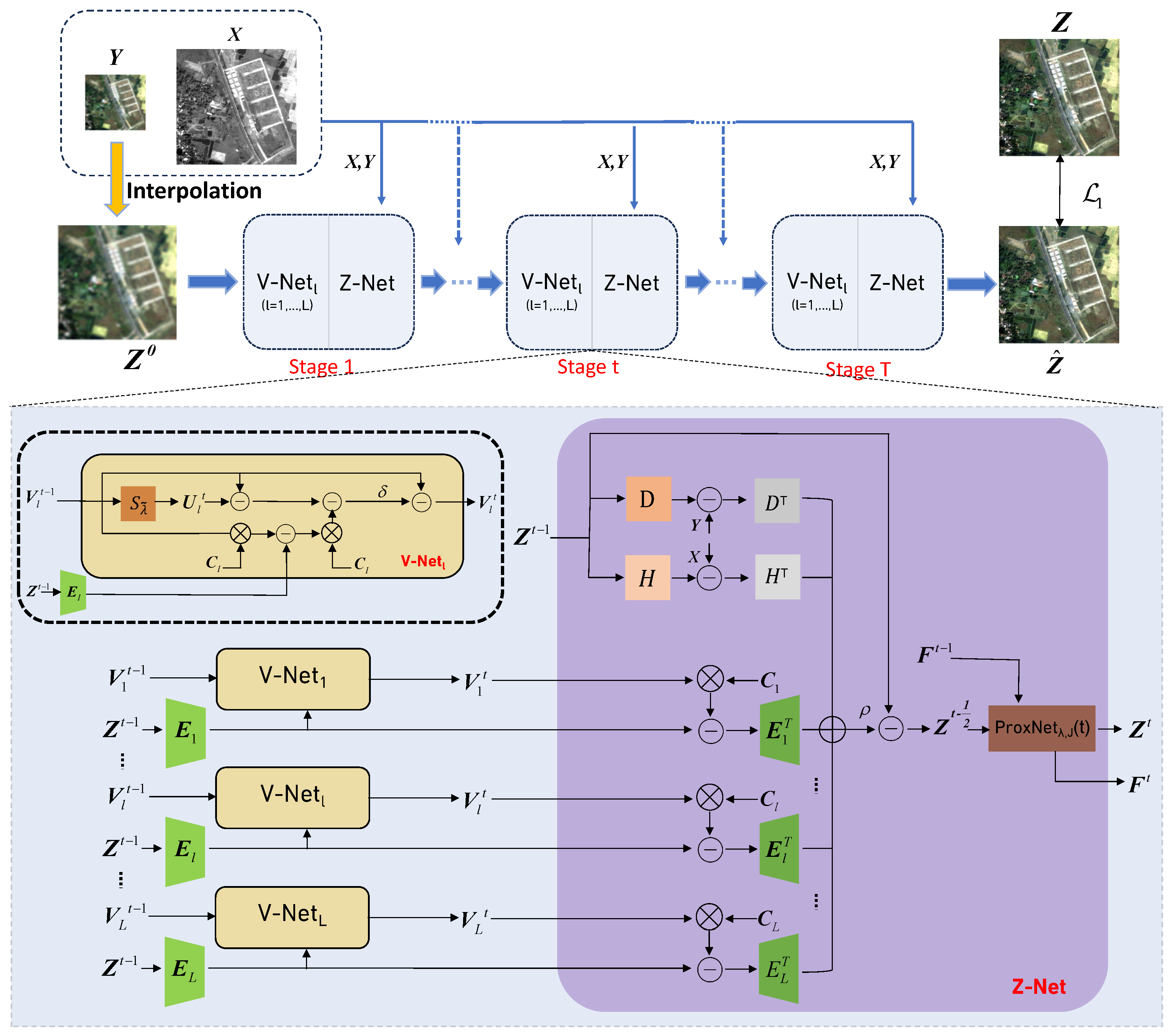
To execute Algorithm 1, massive iterations are necessary, imposing a significant computational burden. Taking advantage of the widespread adoption and rapid development of CNN methods, we deploy our iterative optimization algorithm through deep unrolling neural networks. The overall structure of our proposed DPDU-Net is illustrated in Figure 1, which comprises T stages. Each stage consists of a V-Net and a Z-Net, which will be introduced in detail subsequently. Note that all the modules within each iteration share the same parameters to maintain the physical interpretability of the model. Before the iteration, we interpolate the LRMS image to obtain the initialization of Z . Upon traversing all T stages, the output image Z T will be regarded as the final desired HRMS image.

3.2.1. Network Architecture

We design the V-Net based on the updating rule of the V-subproblem as indicated in Equations (7)–(9). Specifically, the V-Net of t t h iteration takes { V l t 1 } l = 1 L and Z t 1 as inputs and outputs { V l t } l = 1 L . We calculate the auxiliary variable { U l t } l = 1 L through a soft thresholding operation denoted by S λ according to Equation (7). Note that V l t and U l t are the tensor form stacked by { V l k t } k = 1 K and { U l k t } k = 1 K .
Similarly, we implement the Z-Net based on the iteration of the Z-subproblem as indicated in Equations (11)–(13). The Z-Net at the t t h iteration inputs { V l t } l = 1 L , Z t 1 , X , Y and outputs Z t , where { V l t } l = 1 L is the output of the preceding V-Net. The Z-Net involves six CNN modules to simulate the spatial and spectral degradation (i.e., H and D), sparse space transformation (i.e., { E l } l = 1 L ), and corresponding inverse procedures of these processes (i.e., H T , D T and { D l } l = 1 L ). In addition, a ProxNet is used to approximate the proximal operator in traditional optimization methods.
In our implementation, the weight parameters γ , μ , λ , and the step size σ , ρ are learnable and updated through backpropagation during training, while elementary mathematical computations (i.e., add, subtract, ∇, sign ( · ) , and max ( · ) ) are realized directly.

3.2.2. Details of the Degradation and Transformation Modules

We design simple three-layer CNNs to simulate spatial and spectral degradation (i.e., H and D), and the inverse operations of these are implemented using symmetrical structures. The spectral degradation operator H, as outlined in Table 1, carries out a linear operation to decrease the spectral bands from B to a single band. This operation is facilitated by three 3 × 3 convolutional layers. Each of these layers has a stride and padding set to 1, with ReLU activation functions enhancing the first two layers with nonlinearity. Different from the spectral degradation, the spatial degradation operator D involves downsampling followed by blurring. It is achieved by employing three 3 × 3 convolutional layers, with downsampling along the spatial axes performed by the first and last layers through a stride of 2, yielding a total scaling factor of 4.
We show the architecture of the transformation operator { E l } l = 1 L and its inverse operation { E l T } l = 1 L in Figure 2. The transformation operator employs a multi-scale encoder-like architecture, which facilitates the conversion of input images into L-scale feature map space. Each scale within the network comprises a 3 × 3 convolutional layer followed by a residual block. A stride of 2 is employed in every convolutional layer, aside from E 1 , to reduce the spatial resolution of the feature maps. The inverse operation { E l T } l = 1 L mirrors the structure of the transformation operator { E l } l = 1 L , exhibiting a symmetrical multi-scale decoder-like architecture.

3.2.3. ProxNet

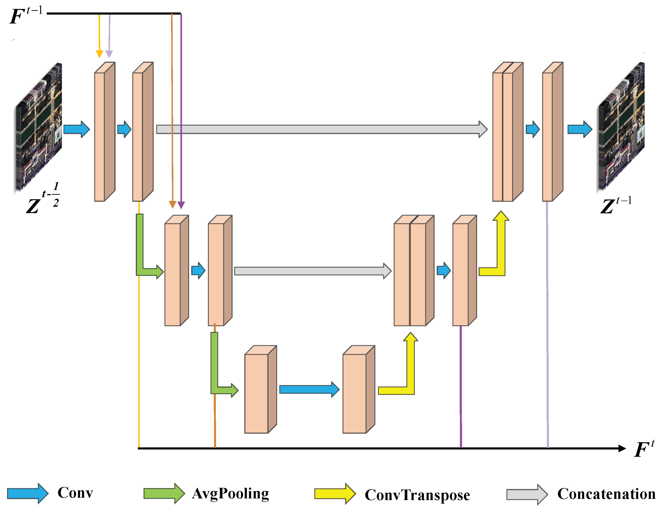
The architecture of the ProxNet is shown in Figure 3. For the t t h iteration, the ProxNet takes Z t 1 2 as input and produces Z t as output. To balance efficiency with performance, we have chosen the widely used U-Net [36] architecture with skip connections as the backbone of ProxNet. The U-Net backbone is structured with an encoder and a decoder that are symmetrical, each consisting of three blocks. Each block integrates two convolutional layers with 3 × 3 kernels and ReLU activation. The encoder uses average pooling to downscale the feature maps, and the decoder uses bilinear interpolation for a two-times upsampling.
This ProxNet enables the learning of features at different resolutions. The feature maps of the same resolution in both the encoder and decoder are concatenated through skip connections, facilitating improved results. Moreover, to enhance the inter-stage information flow, we transmit information from previous stages to the current stage, as depicted by F in Figure 3, where feature maps of the same resolution are connected to achieve effective inter-stage information fusion. This approach ensures the continuity and integrity of information throughout the network.

3.3. Loss Function

Our proposed DPDU-Net is guided by the labeled HRMS images. To achieve the fusion goal, we concentrate on minimizing the mean absolute error (MAE) loss, which is computed using the GT image Z and the generated HRMS image Z ^ . It can be represented as
L l o s s = Z ^ Z 1 .

4. Results

This section encompasses an in-depth evaluation and extensive experimental work to assess the efficacy of the DPDU-Net that we have put forward.

4.1. Experiment Settings

4.1.1. Datasets

Our experiment utilized datasets from two satellites: the GF2 dataset with four MS channels and the WV3 dataset with eight MS channels. The GF2 dataset provided a total of 19,044 groups of images, while the WV3 dataset contributed 10,794 groups. As GT data were unavailable we followed Wald’s protocol and downsampled the PAN and MS images captured at their original resolution by a scale factor of 4 to obtain input image pa. The original MS images served as the GT. Subsequently, we cropped the GT and the downsampled PAN and MS images to sizes of 64 × 64, 64 × 64 and 16 × 16, respectively. The images were subsequently partitioned into training and validation datasets using a 90% to 10% ratio. For testing purposes, we used 20 groups of independently obtained images.

4.1.2. Evaluation Metrics

In addition to the subjective visual comparison, we also used a set of metrics to assess the effectiveness of the proposed DPDU-Net. For the reduced-resolution experiments, we employed five commonly used metrics: spatial correlation coefficient (SCC), spectral angle mapper (SAM), peak signal-to-noise ratio (PSNR), erreur relative globale adimensionnellede synthèse (ERGAS), and the universal image quality index, denoted by Q 2 n , where Q 4 corresponds to MS images with four bands and Q 8 corresponds to MS images with eight bands. For the full-resolution evaluation, in the absence of GT, we utilized the quality with no reference (QNR) metric consisting of D λ for spectral and D s for spatial distortion assessment; both D λ and D s aim for zero, and a QNR index approaches one for better reconstructed image quality.

4.1.3. Implementation Details

In our implementation, we employed the PyTorch 2.1.2 framework and utilized one NVIDIA GeForce RTX 3090 GPU from the United States (Santa Clara, CA, USA) for both training and testing. The network was executed in five stages ( T = 5 ). During training, we employed the Adam optimization algorithm to update the network’s parameters, with a weight decay of 1 × 10 4 and momentum of 0.9. The learning rate was set to 0.001 for the WV3 dataset and to 0.0002 for the GF2 dataset at the beginning. The training involved a total of 500 epochs, during which the learning rate was reduced by half at epochs 100 and 300.

4.2. Comparison Analysis

To comprehensively assess the performance of the proposed model, we compared it with 10 SOTA methods. Specifically, we included five traditional methods, i.e., BDSD [37], PRACS [4], SFIM [38], and MTF-GLP [39], as well as five CNN-based methods, i.e., MSDCNN [9], PanCSC [13], DMDNet [10], MUCNN [11], and LACNet [12]. Furthermore, we also considered the directly upsampled LRMS image, i.e., EXP. We conducted qualitative and quantitative analyses at both reduced resolution and full resolution.
4.2.1. Reduced-Resolution Evaluation

To begin, we performed reduced-resolution evaluations on both the GF2 and WV3 datasets. In the testing phase, we randomly selected 20 pairs of LRMS/PAN images from each dataset. The LRMS images were within dimensions of 64 × 64 , while the PAN images were within dimensions of 256 × 256 .
Quantitative analysis: We show the average value of all five metrics in Table 2 for the GF2 dataset and in Table 3 for the WV3 dataset. As can be seen, EXP, which directly upsampled the LRMS image to the spatial resolution of the HRMS image, achieved the worst results among all the methods. In general, CNN-based approaches outperformed traditional methods, showcasing their superiority, in terms of performance. Among them, the proposed DPDU-Net performed best on all five metrics. Although LACNet achieved the second-best results, its PSNR value was 0.45 dB lower than ours on the WV3 dataset, and the gap was even more significant on the GF2 dataset, reaching 2.06 dB. This highlights the superiority of the DPDU-Net in producing pansharpening results that closely resemble the HRMS reference image in both spectral and spatial characteristics.
Qualitative analysis: Next, we performed a qualitative analysis to assess the performance of the models by visualizing the reconstructed images and their corresponding error images. For the purpose of visualization, we selected the RGB channels to display the result images and the corresponding error maps. As shown in Figure 4 and Figure 5, traditional methods exhibit spectral distortion and a loss of spatial details during image reconstruction. The EXP method generates results with significant ambiguity. Meanwhile, CNN-based methods improve the reconstruction outcomes, making it challenging to distinguish between the reconstructed images and the HRMS reference images. However, upon careful examination of the error images in Figure 6 and Figure 7, we observe that even CNN methods still exhibit discrepancies in preserving spectral and spatial features. In contrast, our proposed method excels in reconstructing both spectral information and spatial details, thereby demonstrating its superiority over other SOTA methods, in terms of visual representation.

4.2.2. Full-Resolution Experiment

We then conducted full-resolution evaluations on the GF2 and WV3 datasets. In the testing phase, we randomly selected 20 pairs of LRMS/PAN images from each dataset. The LRMS images were within dimensions of 64 × 64 , while the PAN images were within dimensions of 256 × 256 .
Quantitative analysis: The results of all three evaluation indicators are shown in Table 4 and Table 5. In general, the CNN-based methods outperformed traditional methods, with the exception of D λ on the WV3 dataset. Among the CNN-based methods, our proposed DPDU-Net demonstrated superior performance, particularly in preserving spectral information on the GF2 dataset and preserving spacial information on the WV3 dataset. Additionally, DPDU-Net achieved the best performance in the comprehensive metric QNR. These results highlight the strength of DPDU-Net in full-resolution experiments. It not only excels in restoring spectral information but also maintains spatial structure without significant distortion.
Qualitative analysis: We visualize the reconstructed images of all models at full resolution in Figure 8 and Figure 9. Since the GT is unavailable, the PAN image serves as a basic image to observe the spatial information. It is evident that traditional methods perform reasonably well in preserving spectral information for WV3 datasets; however, they inevitably introduce substantial spatial distortions. This observation aligns with the findings from our quantitative experiments. Additionally, upon closer examination of the enlarged area, we can observe that the image reconstructed by the CNN-based method exhibits clearer details of the roof, highlighting its superior performance in preserving spatial information compared to traditional methods. In contrast, the proposed DPDU-Net not only effectively recovers spectral information but also maintains spatial information similar to the PAN image. This demonstrates its ability to successfully accomplish the pansharpening task in full-resolution experiments.

4.3. Ablation Experiments

For this section, we performed a series of ablation studies on the GF2 dataset at reduced resolution, to discuss each component of our proposed DPDU-Net. For simplicity, we used the same experimental settings as those in Section 4.2.1.

4.3.1. Analysis on the Double Priors

Our proposed model leverages two complementary priors to enhance performance: an implicit prior combined with a semi-implicit prior. To illustrate the necessity of using double priors, we conducted ablation experiments, and the results are presented in Table 6. Config. I is the model used in our proposed DPDU-Net, incorporating both two priors. In Config. II, only the deep implicit prior is employed, which is a common practice in other deep unrolling methods. Compared to Config. I, the metrics of Config. II showed a slightly better performance, in terms of the ERGAS metric, but the other four metrics were relatively worse. This clearly highlights the importance of incorporating additional semi-implicit priors. In Config. III, only the semi-implicit prior was utilized. Except for the Q4 metric, there was a notable decline in the results of the other four metrics. The reason could be attributed to the fact that deep implicit priors form the foundation of deep unrolling methods, and the absence of such priors hinders the learning of useful information from a large amount of input data. Based on the comprehensive analysis, it can be concluded that using only deep implicit priors already yields relatively good results. However, additional improvement can be achieved by further incorporating semi-implicit priors. Both of these priors complement each other and are essential for achieving optimal performance.

4.3.2. Analysis on the Multi-Scale Implicit Space

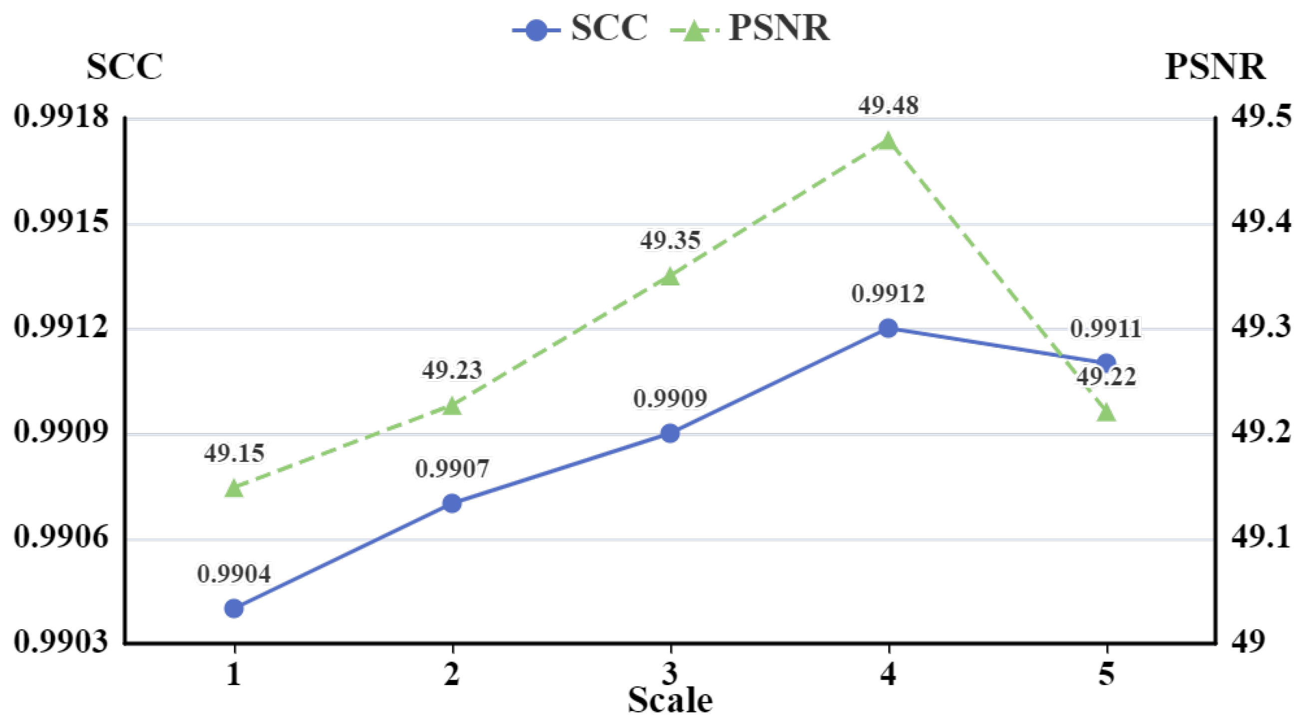
Many existing image reconstruction tasks are accomplished by implementing CSC in the explicit image domain. To obtain a better sparse representation, we introduced a learnable transformation operator to transform the latent HRMS images into implicit spaces and adopt multi-scale convolutions to sparsely encode them separately. To validate the effectiveness of this strategy and determine the optimal number of scales, we conducted comparison experiments with different scales and plotted the line chart of the PSNR/SCC against scale in Figure 10.
As depicted in Figure 10, when the scale was set to 0 (i.e., CSC performed directly in the image domain rather than implicit space) both the PSNR and SCC were at their worst. Introducing the transformation operator and mapping the HRMS image to be reconstructed into a single-scale implicit space for CSC (i.e., 1-scale) resulted in a moderate improvement in PSNR and SCC. This improvement confirms the effectiveness of the semi-implicit prior.
To further enhance the performance of the semi-implicit prior, instead of using a single-scale implicit space, we mapped the HRMS image into a multi-scale implicit space using the encoder-like architecture E l l = 1 L . As observed in Figure 10, increasing the scale beyond 1 led to a gradual improvement in performance, indicating the effectiveness of the multi-scale implicit space. However, when the number of scales exceeded 3, the PSNR and SCC plateaued or even decreased. The reason for the performance drop may lie in the fact that features extracted by deeper networks tend to be highly abstract and complex, which can make them less suitable for sparse representation. Specifically, as the network becomes deeper, the hierarchical layers capture increasingly complex and high-level concepts, resulting in a loss of fine-grained details and local information, which are crucial for accurate sparse representation. This abstraction can lead to challenges in effectively capturing the sparse structure of the data, as the inherent sparsity may not be fully preserved in the deeper feature representations. Consequently, the performance of sparse representation-based methods can be compromised when applied to features extracted from deep networks, as the assumptions underlying the sparse representation model may not hold as strongly. Consequently, we selected a 3-scale implicit sparse space for training the proposed DPDU-Net, i.e., L = 3 , as it achieves the best results.

4.3.3. Analysis on the Number of Stages

Deep unrolling embeds the iterative optimization algorithm into networks, each stage corresponding to an iteration of the algorithm. To select an appropriate number of stages for the proposed DPDU-Net, we conducted comparison experiments with different numbers of stages. The PSNR and SCC values of the different numbers of stages are plotted in Figure 11. It is evident that as the number of stages increased, there was an initial upward trend in the performance. However, after reaching 6 stages, the PSNR and SCC value reach an optimal level and stabilized thereafter. Taking into consideration both performance and efficiency, we determined that 6 stages was the optimal number for the proposed DPDU-Net model, i.e., T = 6 .

4.3.4. Ablation Study about the ProxNet

To further analyze the impact of the inter-stage skip connection of the ProxNet, we conducted an ablation experiment. The results are presented in Table 7, where we compared the performance of the ProxNet with and without the inter-stage information flow (ISIF). It can be observed that introducing ISIF led to an increase in PSNR value, from 48.56 to 49.48. This improvement highlights the effectiveness of the inter-stage skip connection, which enhances overall performance.

5. Discussion

Our proposed DPDU-Net was inspired by PanCSC [13] and SCSC-PNN [15]. Although the two CSC-based unrolling pansharpening (CSC-UP) methods and our method both utilize the CSC theory and are based on the deep unrolling framework, there are two main differences:
  • CSC-UP methods concentrate on modeling input images, specifically the PAN and LRMS images, utilizing CSC to decompose the input images into informative components, and, finally, reconstructing the pansharpened result based on the decomposed features. On the other hand, our method employs CSC to model the sparse representation of the latent HRMS image.
  • CSC-UP methods directly perform sparse coding in the image domain, while our method performs sparse coding on the image features in a latent space.

6. Conclusions

This paper proposed a double prior deep unrolling network (DPDU-Net) for pansharpening. We first introduced a novel pansharpening model that combines an implicit prior and a semi-implicit prior. The semi-implicit prior was achieved by mapping the latent image to a multi-scale implicit space and leveraging convolutional sparse encoding to obtain a more refined sparse representation. We then unrolled the optimization algorithms into a CNN architecture, enabling end-to-end reconstruction. Through extensive experiments conducted on the GF2 and WV3 datasets, our proposed model consistently outperformed other state-of-the-art methods. These results highlight the superiority of the DPDU-Net and affirm its effectiveness in achieving high-quality pansharpening outcomes.
Through the analysis of the experiments, it can be observed that learning-based methods suffer from slightly poor generalization. Specifically, when models trained on reduced-resolution datasets are applied to full-resolution evaluation, their performance tends to degrade to varying degrees. In future work, we plan to investigate this issue further by exploring techniques such as semi-supervised or unsupervised training, to mitigate the generalization problem.

Author Contributions

Conceptualization, Y.L.; methodology, Y.C. (Yingxia Chen); validation, Y.L.; writing—original draft preparation, Y.C. (Yingxia Chen); writing—review and editing, T.W.; supervision, Y.C. (Yan Chen) and F.F.; funding acquisition, Y.C. (Yan Chen) and F.F. All authors have read and agreed to the published version of the manuscript.

Funding

This work was supported by Shanghai Key Laboratory of Multidimensional Information Processing, East China Normal University under Grant MIP20222, in part by the National Natural Science Foundation of China under Grant 62202173, in part by the Fundamental Research Funds for the Central Universities, in part by the China University Industry-University-Research Innovation Fund Project under Grant 2021RYC06002 and in part by the Scientific Research Program of Hubei Provincial Department of Education under Grant B2022040.

Data Availability Statement

Data are contained within the article.

Conflicts of Interest

The authors declare no conflicts of interest. The funders had no role in the design of the study; in the collection, analyses, or interpretation of data; in the writing of the manuscript; or in the decision to publish the results.

References

  1. Laben, C.A.; Brower, B.V. Process for Enhancing the Spatial Resolution of Multispectral Imagery Using Pan-Sharpening. US Patent 6,011,875, 4 January 2000. [Google Scholar]
  2. Ghahremani, M.; Ghassemian, H. Nonlinear IHS: A Promising Method for Pan-Sharpening. IEEE Geosci. Remote Sens. Lett. 2016, 13, 1606–1610. [Google Scholar] [CrossRef]
  3. Duran, J.; Buades, A. Restoration of Pansharpened Images by Conditional Filtering in the PCA Domain. IEEE Geosci. Remote Sens. Lett. 2018, 16, 442–446. [Google Scholar] [CrossRef]
  4. Choi, J.; Yu, K.; Kim, Y. A New Adaptive Component-Substitution-Based Satellite Image Fusion by Using Partial Replacement. IEEE Trans. Geosci. Remote Sens. 2011, 49, 295–309. [Google Scholar] [CrossRef]
  5. Khan, M.M.; Chanussot, J.; Condat, L.; Montanvert, A. Indusion: Fusion of Multispectral and Panchromatic Images Using the Induction Scaling Technique. IEEE Geosci. Remote Sens. Lett. 2008, 5, 98–102. [Google Scholar] [CrossRef]
  6. Li, H.; Liu, F.; Yang, S.; Zhang, K.; Su, X.; Jiao, L. Refined Pan-Sharpening With NSCT and Hierarchical Sparse Autoencoder. IEEE J. Sel. Top. Appl. Earth Obs. Remote Sens. 2016, 9, 5715–5725. [Google Scholar] [CrossRef]
  7. Masi, G.; Cozzolino, D.; Verdoliva, L.; Scarpa, G. Pansharpening by Convolutional Neural Networks. Remote Sens. 2016, 8, 594. [Google Scholar] [CrossRef]
  8. Yang, J.; Fu, X.; Hu, Y.; Huang, Y.; Ding, X.; Paisley, J. PanNet: A Deep Network Architecture for Pan-Sharpening. In Proceedings of the IEEE International Conference on Computer Vision, Venice, Italy, 22–29 October 2017; pp. 5449–5457. [Google Scholar]
  9. Jianwen, H.; Pei, H.; Kang, X.; Zhang, H.; Fan, S. Pan-Sharpening via Multiscale Dynamic Convolutional Neural Network. IEEE Trans. Geosci. Remote Sens. 2021, 59, 2231–2244. [Google Scholar]
  10. Fu, X.; Wang, W.; Huang, Y.; Ding, X.; Paisley, J.W. Deep Multiscale Detail Networks for Multiband Spectral Image Sharpening. IEEE Trans. Neural Netw. Learn. Syst. 2020, 32, 2090–2104. [Google Scholar] [CrossRef] [PubMed]
  11. Wang, Y.; Deng, L.J.; Zhang, T.J.; Wu, X. SSconv: Explicit Spectral-to-Spatial Convolution for Pansharpening. In Proceedings of the 29th ACM International Conference on Multimedia, Virtual Event, 20–24 October 2021. [Google Scholar]
  12. Jin, Z.R.; Zhang, T.J.; Jiang, T.X.; Vivone, G.; Deng, L.J. LAGConv: Local-Context Adaptive Convolution Kernels with Global Harmonic Bias for Pansharpening. In Proceedings of the AAAI Conference on Artificial Intelligence, Online, 22 February–1 March 2022. [Google Scholar]
  13. Cao, X.; Fu, X.; Hong, D.; Xu, Z.; Meng, D. PanCSC-Net: A Model-Driven Deep Unfolding Method for Pansharpening. IEEE Trans. Geosci. Remote Sens. 2021, 60, 1–13. [Google Scholar] [CrossRef]
  14. Yang, G.; Zhou, M.; Yan, K.; Liu, A.; Fu, X.; Wang, F. Memory-augmented Deep Conditional Unfolding Network for Pansharpening. In Proceedings of the IEEE/CVF Conference on Computer Vision and Pattern Recognition, New Orleans, LA, USA, 18–24 June 2022; pp. 1788–1797. [Google Scholar]
  15. Xu, S.; Zhang, J.; Sun, K.; Zhao, Z.; Huang, L.; Liu, J.; Zhang, C. Deep Convolutional Sparse Coding Network for Pansharpening with Guidance of Side Information. In Proceedings of the 2021 IEEE International Conference on Multimedia and Expo, Shenzhen, China, 5–9 July 2021; IEEE: Piscataway, NJ, USA, 2021; pp. 1–6. [Google Scholar]
  16. Wu, Z.C.; Huang, T.; Deng, L.J.; Hu, J.F.; Vivone, G. VO+Net: An Adaptive Approach Using Variational Optimization and Deep Learning for Panchromatic Sharpening. IEEE Trans. Geosci. Remote Sens. 2022, 60, 1–16. [Google Scholar] [CrossRef]
  17. Wang, H.; Gong, M.; Mei, X.; Zhang, H.; Ma, J. Deep Unfolded Network with Intrinsic Supervision for Pan-Sharpening. In Proceedings of the AAAI Conference on Artificial Intelligence, Vancouver, BC, Canada, 20–27 February 2024. [Google Scholar]
  18. Feng, Y.; Liu, J.; Chen, K.; Wang, B.; Zhao, Z. Optimization Algorithm Unfolding Deep Networks of Detail Injection Model for Pansharpening. IEEE Geosci. Remote Sens. Lett. 2021, 19, 1–5. [Google Scholar] [CrossRef]
  19. Tian, X.; Li, K.; Wang, Z.; Ma, J. VP-Net: An Interpretable Deep Network for Variational Pansharpening. IEEE Trans. Geosci. Remote Sens. 2021, 60, 1–16. [Google Scholar] [CrossRef]
  20. Ballester, C.; Caselles, V.; Igual, L.; Verdera, J.; Rougé, B. A Variational Model for P+XS Image Fusion. Int. J. Comput. Vis. 2006, 69, 43–58. [Google Scholar] [CrossRef]
  21. Möller, M.; Wittman, T.; Bertozzi, A.L.; Burger, M. A Variational Approach for Sharpening High Dimensional Images. SIAM J. Imaging Sci. 2012, 5, 150–178. [Google Scholar] [CrossRef]
  22. Fang, F.; Li, F.; Shen, C.; Zhang, G. A Variational Approach for Pan-Sharpening. IEEE Trans. Image Process. 2013, 22, 2822–2834. [Google Scholar] [CrossRef] [PubMed]
  23. Ding, X.; Jiang, Y.; Huang, Y.; Paisley, J. Pan-Sharpening with a Bayesian Nonparametric Dictionary Learning Model. In Proceedings of the Artificial Intelligence and Statistics, Reykjavik, Iceland, 22–25 April 2014; PMLR: New York, NY, USA, 2014; pp. 176–184. [Google Scholar]
  24. Wang, T.; Fang, F.; Li, F.; Zhang, G. High-Quality Bayesian Pansharpening. IEEE Trans. Image Process. 2018, 28, 227–239. [Google Scholar] [CrossRef] [PubMed]
  25. Liu, X.; Liu, Q.; Wang, Y. Remote Sensing Image Fusion Based on Two-Stream Fusion Network. Inf. Fusion 2020, 55, 1–15. [Google Scholar] [CrossRef]
  26. Sun, Q.; Sun, Y.; Pan, C. AIDB-Net: An Attention-Interactive Dual-Branch Convolutional Neural Network for Hyperspectral Pansharpening. Remote Sens. 2024, 16, 1044. [Google Scholar] [CrossRef]
  27. Gao, Y.; Qin, M.; Wu, S.; Zhang, F.; Du, Z. GSA-SiamNet: A Siamese Network with Gradient-Based Spatial Attention for Pan-Sharpening of Multi-Spectral Images. Remote Sens. 2024, 16, 616. [Google Scholar] [CrossRef]
  28. Liu, Q.; Zhou, H.; Xu, Q.; Liu, X.; Wang, Y. PSGAN: A Generative Adversarial Network for Remote Sensing Image Pan-Sharpening. IEEE Trans. Geosci. Remote Sens. 2020, 59, 10227–10242. [Google Scholar] [CrossRef]
  29. Ma, J.; Yu, W.; Chen, C.; Liang, P.; Guo, X.; Jiang, J. Pan-GAN: An Unsupervised Pan-Sharpening Method for Remote Sensing Image Fusion. Inf. Fusion 2020, 62, 110–120. [Google Scholar] [CrossRef]
  30. Zeiler, M.D.; Krishnan, D.; Taylor, G.W.; Fergus, R. Deconvolutional Networks. In Proceedings of the 2010 IEEE Computer Society Conference on Computer Vision and Pattern Recognition, San Francisco, CA, USA, 13–18 June 2010; pp. 2528–2535. [Google Scholar]
  31. Zeiler, M.D.; Taylor, G.W.; Fergus, R. Adaptive Deconvolutional Networks for Mid and High Level Feature Learning. In Proceedings of the International Conference on Computer Vision, Barcelona, Spain, 6–13 November 2011; pp. 2018–2025. [Google Scholar]
  32. Li, M.; Xie, Q.; Zhao, Q.; Wei, W.; Gu, S.; Tao, J.; Meng, D. Video Rain Streak Removal by Multiscale Convolutional Sparse Coding. In Proceedings of the IEEE/CVF Conference on Computer Vision and Pattern Recognition, Salt Lake, UT, USA, 18–23 June 2018; pp. 6644–6653. [Google Scholar]
  33. Deng, X.; Liu, E.; Li, S.; Duan, Y.; Xu, M. Interpretable Multi-Modal Image Registration Network Based on Disentangled Convolutional Sparse Coding. IEEE Trans. Image Process. 2023, 32, 1078–1091. [Google Scholar] [CrossRef] [PubMed]
  34. Wang, H.; Xie, Q.; Zhao, Q.; Meng, D. A Model-Driven Deep Neural Network for Single Image Rain Removal. In Proceedings of the 2020 IEEE/CVF Conference on Computer Vision and Pattern Recognition, Seattle, WA, USA, 13–19 June 2020; pp. 3100–3109. [Google Scholar]
  35. Wang, H.; Xie, Q.; Li, Y.; Huang, Y.; Meng, D.; Zheng, Y. Orientation-Shared Convolution Representation for CT Metal Artifact Learning. In Proceedings of the International Conference on Medical Image Computing and Computer-Assisted Intervention, Vancouver, BC, Canada, 8–12 October 2022. [Google Scholar]
  36. Ronneberger, O.; Fischer, P.; Brox, T. U-Net: Convolutional Networks for Biomedical Image Segmentation. In Proceedings of the International Conference on Medical Image Computing and Computer-Assisted Intervention, Toronto, ON, Canada, 18–22 September 2015; Springer: Berlin/Heidelberg, Germany, 2015; pp. 234–241. [Google Scholar]
  37. Garzelli, A.; Nencini, F.; Capobianco, L. Optimal MMSE Pan Sharpening of Very High Resolution Multispectral Images. IEEE Trans. Geosci. Remote Sens. 2008, 46, 228–236. [Google Scholar] [CrossRef]
  38. Schowengerdt, R.A. Remote Sensing, Models, and Methods for Image Processing; Elsevier: Amsterdam, The Netherlands, 1997. [Google Scholar]
  39. Aiazzi, B.; Alparone, L.; Baronti, S.; Garzelli, A.; Selva, M. MTF-tailored Multiscale Fusion of High-resolution MS and Pan Imagery. Photogramm. Eng. Remote Sens. 2006, 72, 591–596. [Google Scholar] [CrossRef]
Figure 1. The overall framework of the proposed DPDU-Net. It iterates T stages, each consisting of a V-Net and a Z-Net.
Remotesensing 16 02141 g001
Figure 2. The detailed architecture of the transformation operator { E l } l = 1 L and its inverse operation { E l T } l = 1 L .
Remotesensing 16 02141 g002
Figure 3. The detailed architecture of the proposed ProxNet. For the t t h iteration, the ProxNet takes Z t 1 2 as input and produces Z t as output.
Remotesensing 16 02141 g003
Figure 4. Visual results of qualitative comparisons on the reduced-resolution GF2 dataset. The regions of interest in the image, which were framed, have been enlarged and displayed in the lower left and lower right corners, respectively.
Remotesensing 16 02141 g004
Figure 5. Visual results of qualitative comparisons on the reduced-resolution WV3 dataset. The regions of interest in the image, which were framed, have been enlarged and displayed in the lower left and lower right corners, respectively.
Remotesensing 16 02141 g005
Figure 6. Error maps of qualitative comparisons on the reduced-resolution GF2 dataset.
Remotesensing 16 02141 g006
Figure 7. Error maps of qualitative comparisons on the reduced-resolution WV3 dataset.
Remotesensing 16 02141 g007
Figure 8. Visual results of qualitative comparisons on the full-resolution GF2 dataset. The regions of interest in the image, which were framed, have been enlarged and displayed in the lower left and lower right corners, respectively.
Remotesensing 16 02141 g008
Figure 9. Visual results of qualitative comparisons on the full-resolution WV3 dataset. The regions of interest in the image, which were framed, have been enlarged and displayed in the lower left and lower right corners, respectively.
Remotesensing 16 02141 g009
Figure 10. The line chart of the PSNR/SCC against scale. The vertical axis represents the evaluation indicators PSNR and SCC, with higher values indicating better performance, and the horizontal axis indicates the number of scales used in the CSC methods (0-scales indicates that the CSC method was performed directly in the image domain).
Remotesensing 16 02141 g010
Figure 11. The line chart of the PSNR/SCC against stage. The vertical axis represents the evaluation indicators PSNR and SCC, with higher values indicating better performance, and the horizontal axis indicates the number of stages in the deep unrolling network.
Remotesensing 16 02141 g011
Table 1. The detailed architecture of the H , H T , D , D T . All convolutional filter sizes are set to 3 × 3 .
OperationResamplein_Channelout_ChannelNonlinearity
HConv Layerstride-1B32ReLU
Conv Layerstride-13232ReLU
Conv Layerstride-1321-
H T Conv Layerstride-1132ReLU
Conv Layerstride-13232ReLU
Conv Layerstride-132B-
DConv Layerstride-2B32ReLU
Conv Layerstride-13232ReLU
Conv Layerstride-232B-
D T ConvTransposestride-2B32ReLU
Conv Layerstride-13232ReLU
ConvTransposestride-232B-
Table 2. Quantitative indices on the reduced-resolution GF2 dataset. The best indicator is highlighted in bold, while the second-best indicator is underlined.
MethodGF-2 Dataset
Q4 ↑ERGAS ↓SAM ↓PSNR ↑SCC ↑
EXP0.79712.40631.852137.960.7896
BDSD0.88421.68831.734540.990.9175
PRACS0.89751.64611.712641.250.913
SFIM0.88491.6971.669240.920.9044
MTF-GLP0.89081.57361.653241.500.9136
PanCSC0.93271.31971.354243.090.9587
MSDCNN0.95571.11091.08844.610.9714
DMDNet0.94291.24931.157343.600.9665
MUCNN0.96540.91781.008246.170.9819
LACNet0.97390.79750.891147.420.9856
Ours0.98240.62820.707649.480.9912
Table 3. Quantitative indices on the reduced-resolution WV3 dataset. The best indicator is highlighted in bold, while the second best indicator is underlined.
MethodWV-3 Dataset
Q4 ↑ERGAS ↓SAM ↓PSNR ↑SCC ↑
EXP0.60277.12895.838127.070.5499
BDSD0.79094.87585.833430.530.8563
PRACS0.77215.21065.614829.940.8165
SFIM0.78225.07745.373230.050.8559
MTF-GLP0.81084.78995.308330.590.8542
PanCSC0.87782.78933.829835.250.9721
MSDCNN0.89012.61073.520235.870.9765
DMDNet0.85273.11984.176034.300.9660
MUCNN0.86282.93574.078434.880.9705
LACNet0.90442.26523.067437.110.9839
Ours0.91512.13622.907737.560.9863
Table 4. Quantitative indices on the full-resolution GF2 dataset. The best indicator is highlighted in bold, while the second best indicator is underlined.
MethodGF2 Dataset
D λ D s QNR ↑
EXP00.15250.8475
BDSD0.03720.05740.9077
PRACS0.06600.06760.8712
MTF-GLP0.09380.08890.8265
SFIM0.06880.04360.8911
PanCSC0.02860.03680.9358
MSDCNN0.02430.03100.9455
DMDNet0.02650.01090.9629
MUCNN0.02360.01270.9640
LACNet0.02710.02510.9485
Ours0.01720.01430.9687
Table 5. Quantitative indices on the full-resolution WV3 dataset. The best indicator is highlighted in bold, while the second best indicator is underlined.
MethodWV3 Dataset
D λ D s QNR ↑
EXP00.09810.9019
BDSD0.04010.09490.8688
PRACS0.02070.06960.9114
MTF-GLP0.03580.05380.9128
SFIM0.02630.04710.9281
PanCSC0.02860.02550.9468
MSDCNN0.03090.03070.9395
DMDNet0.03270.02090.9473
MUCNN0.04310.03550.9232
LACNet0.03140.02330.9461
Ours0.02980.02030.9505
Table 6. Ablation study about the implicit prior (IP) and the semi-implicit prior (SIP). The best indicator is highlighted in bold, while the second-best indicator is underlined.
Config.IPSIPQ4 ↑SAM ↓ERGAS ↓SCC ↑PSNR ↑
I0.98240.62820.70760.991249.48
II×0.98130.75530.66370.990249.03
III×0.98240.97530.84800.986147.32
Table 7. The performance comparison of the ProxNet with or without the inter-stage information flow (ISIF).
ProxNetQ4 ↑SAM ↓ERGAS ↓SCC ↑PSNR ↑
w/o ISIF0.97940.78190.70040.989148.56
with ISIF0.98240.70760.62820.991249.48
Disclaimer/Publisher’s Note: The statements, opinions and data contained in all publications are solely those of the individual author(s) and contributor(s) and not of MDPI and/or the editor(s). MDPI and/or the editor(s) disclaim responsibility for any injury to people or property resulting from any ideas, methods, instructions or products referred to in the content.