Abstract
Cross-domain scene classification requires the transfer of knowledge from labeled source domains to unlabeled target domain data to improve its classification performance. This task can reduce the labeling cost of remote sensing images and improve the generalization ability of models. However, the huge distributional gap between labeled source domains and unlabeled target domains acquired by different scenes and different sensors is a core challenge. Existing cross-domain scene classification methods focus on designing better distributional alignment constraints, but are under-explored for fine-grained features. We propose a cross-domain scene classification method called the Frequency Component Adaptation Network (FCAN), which considers low-frequency features and high-frequency features separately for more comprehensive adaptation. Specifically, the features are refined and aligned separately through a high-frequency feature enhancement module (HFE) and a low-frequency feature extraction module (LFE). We conducted extensive transfer experiments on 12 cross-scene tasks between the AID, CLRS, MLRSN, and RSSCN7 datasets, as well as two cross-sensor tasks between the NWPU-RESISC45 and NaSC-TG2 datasets, and the results show that the FCAN can effectively improve the model’s performance for scene classification on unlabeled target domains compared to other methods.
1. Introduction
Remote sensing (RS) image scene classification [1,2,3,4] aims to infer the semantic labels of a scene, e.g., airports, forests, etc., from a given remote sensing image. It is a challenging task for remote sensing images and has a wide range of real-world applications such as land use [5] and urban planning [6]. Therefore, it has turned into a popular research direction in recent years.
With advances in technology, different types of sensors have greatly enriched the variety and quantity of remote sensing satellite images. In addition, the deep learning method represented by convolutional neural networks (CNNs), which are data-driven, overcomes the difficulties of traditional machine learning methods that require hand-designed features, all of which bring great opportunities for intelligent remote sensing image analysis.
Deep neural networks have enormously improved the performance of remote sensing image scene classification [3,7,8]. However, in practical applications, deep learning algorithms still have several problems. First, their success is due to a large number of high-quality labeled samples. The reliance on professionals for the labeling of remote sensing images, as well as the big data characteristics of remote sensing images, makes the labeling cost higher. Second, supervised learning methods all make the basic assumption that the training data and test data used for the model come from the same distribution. However, in practical applications, this assumption is not always true. In the context of the remote sensing discipline, this further exacerbates the problem of domain shifting [9], where the difference in distribution between two remote sensing images comes from several aspects [10]:
- Differences in the types of sensors and differences in parameters: Due to the differences in the types of sensors, heterogeneous data are produced with huge differences in data modalities, e.g., optical, hyperspectral, infrared, etc. Even sensors of the same modality, such as Gaofen-2 and WorldView satellites, have different resolutions and produce different spectra of images due to parameter differences.
- Differences in imaging conditions: even for the same sensor platform, for the same region, two images collected at different moments have large differences due to the influence of external conditions such as atmospheric conditions, platform attitude, and illumination.
- Scene differences: For the same sensor platform, due to the impact of history, geography and other factors, the same category of scenes contains differences. For example, China and the United States have very different architectural styles.
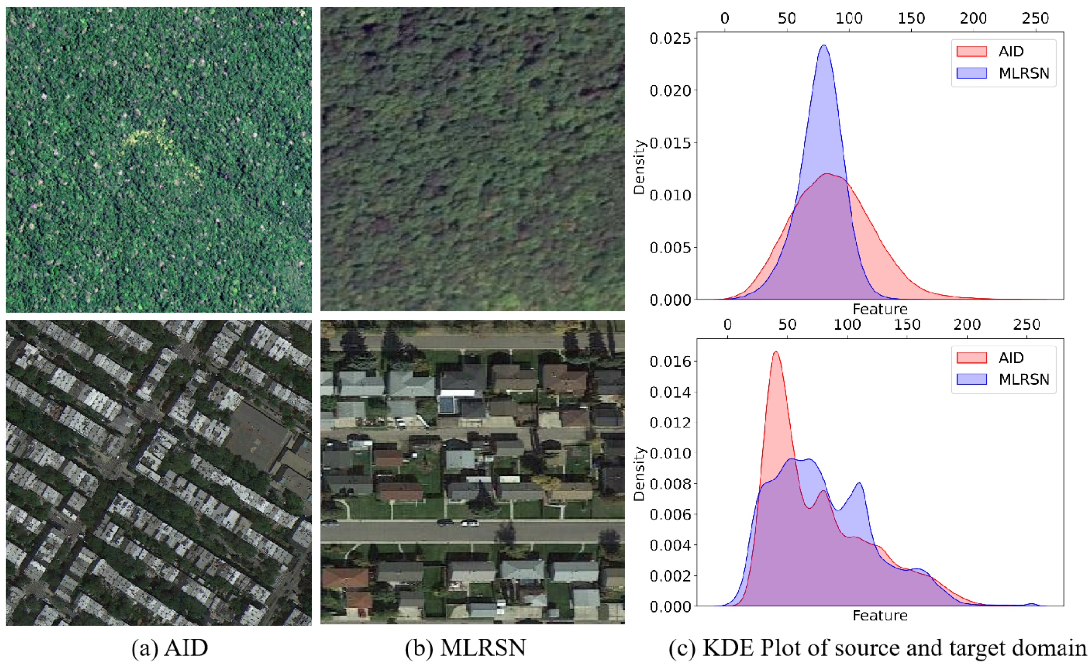
As shown in Figure 1a,b, for images of the same category in the AID and MLRSN datasets, they have different colors, viewpoints and styles, and as shown in Figure 1c, these differences manifest themselves as inconsistencies in the data distribution.
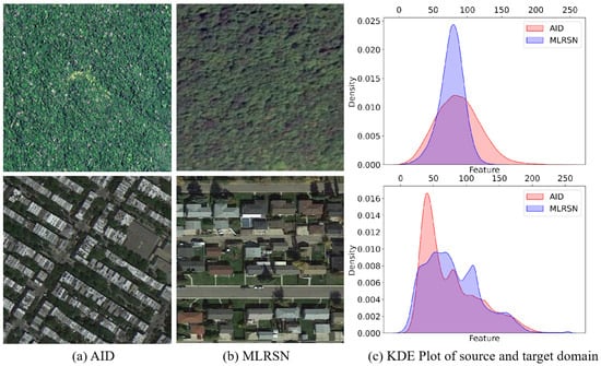
Figure 1.
Examples and intensity distributions of the AID and MLRSN datasets via KDE plots, with “forest” in the first row and “residential area” in the second row.
One feasible technique to solve the above contradiction between big data and less annotations is transfer learning. Works such as [11] introduced transfer learning into the field of remote sensing. As an important research direction in machine learning, transfer learning mines the similarity between the new problem and the original problem to realize the transfer of knowledge. Based on this, researchers proposed a cross-domain scene classification task. Distinguished from the ordinary scene classification task, the cross-domain scene classification task focuses on the model and knowledge transfer between multiple datasets, bridging the gap between data distributions in different domains. It is gratifying to see that some works [12,13] tried to solve the cross-domain scene classification problem with domain adaptation techniques and achieved good results. Domain adaptation (DA) has been a popular approach in transfer learning in recent years, which enabled studies of how to migrate the knowledge learned from a large number of labeled samples to unlabeled samples when sharing the same feature and category space and when the feature distribution changes. Existing cross-domain scene classification methods based on domain adaptation can be mainly categorized into methods based on distribution difference metrics [13,14,15,16,17] and methods based on adversarial learning [18,19,20,21].
However, there are still some problems with the current methods. On the one hand, most DA methods focus on natural images; remote sensing images are more complex and contain more information. Traditional single-feature representation cannot completely describe all the information in the image. On the other hand, existing alignment methods may not be able to completely solve the distributional gap problem; both methods based on distributional difference metrics and methods based on adversarial training focus only on marginal distributional alignment, which reduces the model’s classification performance on the unlabeled target domain. Therefore, characterizing the information in remote sensing images in a more detailed way to alleviate the negative transfer problem due to the complexity of the scene and constructing better distribution-aligned regular terms are the focus of our research.
Article [22] proves that, in the human recognition process, only low-frequency semantic information such as shapes can be utilized for recognition, whereas CNNs simultaneously have the ability to capture high-frequency components that humans cannot perceive. This discovery explains to a certain extent the generalization ability and the anti-sample robustness of CNNs, and also simultaneously explains why the recognition rate of CNNs is higher than that of human beings. For example, it is difficult for human annotators to distinguish between roads and rivers in remote sensing images based only on low-frequency components such as shape features, and they can be further recognized with the help of high-frequency features such as texture and edges.
Inspired by the above phenomenon, in this paper, we propose the Frequency Component Adaptation Network (FCAN) for cross-domain scene classification for remote sensing, which refines the feature representation and separates the low-frequency feature components and high-frequency feature components. Specifically, our proposed method consists of a high-frequency feature branch, a low-frequency feature branch and a classification branch. For the high-frequency branch, a high-frequency feature enhancement module (HFE) is first used for the source and target domains, and the source domain’s high-frequency features are supervised with category labeling information, while the high-frequency features of the source and target domains, both of which are trained adversarially, are supervised with domain labeling information. For the low-frequency branch, a dynamic maximum mean discrepancy (DMMD) loss is used for the distribution alignment of the source domain’s low-frequency features and the target domain’s low-frequency features extracted by the low-frequency feature extraction module (LFE).
In this paper, we can summarize our contributions as follows:
- A novel framework is proposed to decompose the features into low-frequency feature components and high-frequency feature components to be processed separately during the adaptation process, and the two dominant domain adaptation methods, namely, distribution-based and adversarial-based alignment, are organically integrated.
- In order to enhance the intra-domain discriminative ability of the network, we propose a high-frequency feature enhancement module. To enhance the inter-domain generalization ability of the network, better inter-domain invariant features are mined using dynamic MMD loss improved with low-frequency semantic information.
- Extensive transfer experiments on the merged cross-scene dataset and cross-sensor dataset validate the effectiveness of the method. Both our methods outperform several existing cross-domain classification methods.
The rest of the paper is organized as described below. Section 2 describes the literature associated with cross-domain scene classification of remote sensing images. Section 3 describes the architecture of the FCAN and its components in more detail. Section 4 presents the designed experiments and the corresponding experimental results. At last, we conclude this study in Section 5.
2. Related Work
2.1. Domain Adaption
There are two major classes of classical adaptation methods: one based on distributional differences and the other based on adversarial training [23].
Methods based on distribution difference metrics learn the transformation relationship between the source domain features and the target domain features by minimizing the distribution difference between the two domain features, and distribution alignment is realized between the source domain and the target domain. Some common distribution difference metrics have been widely used in the literature and are described in the following. The maximum mean discrepancy (MMD) achieves domain alignment by aligning the sample means of the source and target domain in the regenerated kernel Hilbert space. Based on ordinary classification networks, DDC [24] contains an extra adaptation layer and the MMD-based domain error loss. Considering that DDC only consists of a single-layer network, DAN [25] was introduced to compute the domain error loss for the last three layers of AlexNet, which improved the transfer ability of the network and improved the single kernel function used by DDC in MMD computation to multi-core MMD with a better characterization ability. Unlike marginal distribution alignment methods such as DDC and DAN, JAN [26] further considers the bias of conditional distributions by proposing joint MMD; it was generalized from data adaptation to category adaptation. Considering the fact that category prior distributions in the source and target domains are different, Yan et al. [27] proposed the weighted MMD method. CORAL achieved alignment by approximating the distance between the second-order statistics of the source and target domain distributions, and DeepCORAL [28] introduced CORAL to deep neural networks, which was able to achieve a superior performance over DDC.
Based on the method of adversarial training, the idea of generative adversarial networks (GANs) [29] was borrowed for domain adaptation. Specifically, the process of adversarial learning of the generative and discriminative networks in GANs playing against each other was converted into a game process between the feature extraction network and the domain discriminator network. The domain discriminator was used to discriminate between the source and target domain distributions, enabling the feature extraction network to extract domain-invariant features of a higher quality. DANN [30] includes a gradient reversal layer (GRL) between the feature extractor and the domain discriminator, which is a module that automatically inverts the direction of the gradient during backpropagation. The final domain alignment was achieved to minimize the classification loss and maximize the domain classification loss. CDAN [31] is a conditional distribution adaptation method that uses a multilinear mapping approach to better utilize the results of classification. In contrast, our approach integrates both paradigms in the same framework, fully utilizing the advantages of both.
2.2. Cross-Domain Scene Classification
In recent years, research on the task of RS image scene classification has gradually shifted from a purely supervised learning paradigm to a domain adaptation paradigm. Zhu et al. [13] introduced a method to align both the marginal and conditional distributions simultaneously, and combined an attention mechanism and a multiscale strategy to obtain more robust and complete features. Tao et al. [32] explored the cross-optical sensor task and proposed a transfer transfer learning framework based on multiple intermediate domain transitions. Yang et al. [14] achieved better distributional alignment by dynamically adjusting the comparative importance of the marginal and conditional distributions during the domain alignment process. Zhao et al. [33] focused on the mining of intrinsic associations in the scene by conveying the knowledge of semantic relationships between the source and target domains to effectively boost the model’s performance in the target domain. Focusing on the semi-supervised domain adaptation task, ref. [34] established two regularization constraints, unsupervised comparison and supervised comparison, to achieve a better cross-domain classification performance. Considering the limitations of a single representation, a module capable of obtaining better domain invariant features, through which the sample can be mapped to multiple representations, was proposed [35]. The features were mapped to a Grassmann manifold space for metrics to alleviate the feature degradation problem during the adaptive process [36]. Chen et al. [37] proposed a spatial generalization neural network search framework to solve the cross-domain scene classification problem to bridge the domain gap. Xu et al. [38] mapped the samples to the Lie group manifold space, fusing features of different levels and scales to obtain better domain-invariant features. Meanwhile, an attention mechanism based on dynamic feature fusion alignment was introduced, which effectively enhances the weight of key regions. Zhang et al. [39] used a self-supervised masked image modeling mechanism to improve the discriminative properties of target domain features and used a cluster-centered correction strategy to correct unreliable pseudo-labels, improve the quality of pseudo-labels, and enhance the cross-scene classification performance of target domain classifiers. Unlike the above work, our method considers more refined features in order to cope with complex remote sensing images and achieves more detailed adaptation.
3. Materials and Methods
This section first introduces some definitions and notation for domain adaptation and then describes the proposed FCAN in detail, as well as the internal low-frequency and high-frequency branches, including the corresponding modules and loss functions. Finally, the overall optimization objective is provided.
3.1. Preliminary
We begin by introducing some of the symbols and notation used in this paper. We follow the formulation of [23], where the domain consists of a feature space and a marginal probability distribution , , i.e., . Consider a labeled source domain of samples of , where , and is the label corresponding to the sample , and an unlabeled target domain of samples of , where . The goal of DA is to learn a function such that it minimizes the prediction error on the target domain using data from the source domain, with the same feature space and category space and different joint probability distributions, i.e., , and .
3.2. Overview
In this work, a domain adaptive framework based on feature frequency decomposition is proposed, which is processed separately from two perspectives, the alignment of low-frequency features and the adversarial training of high-frequency features, to achieve better alignment of features in the source and target domains.
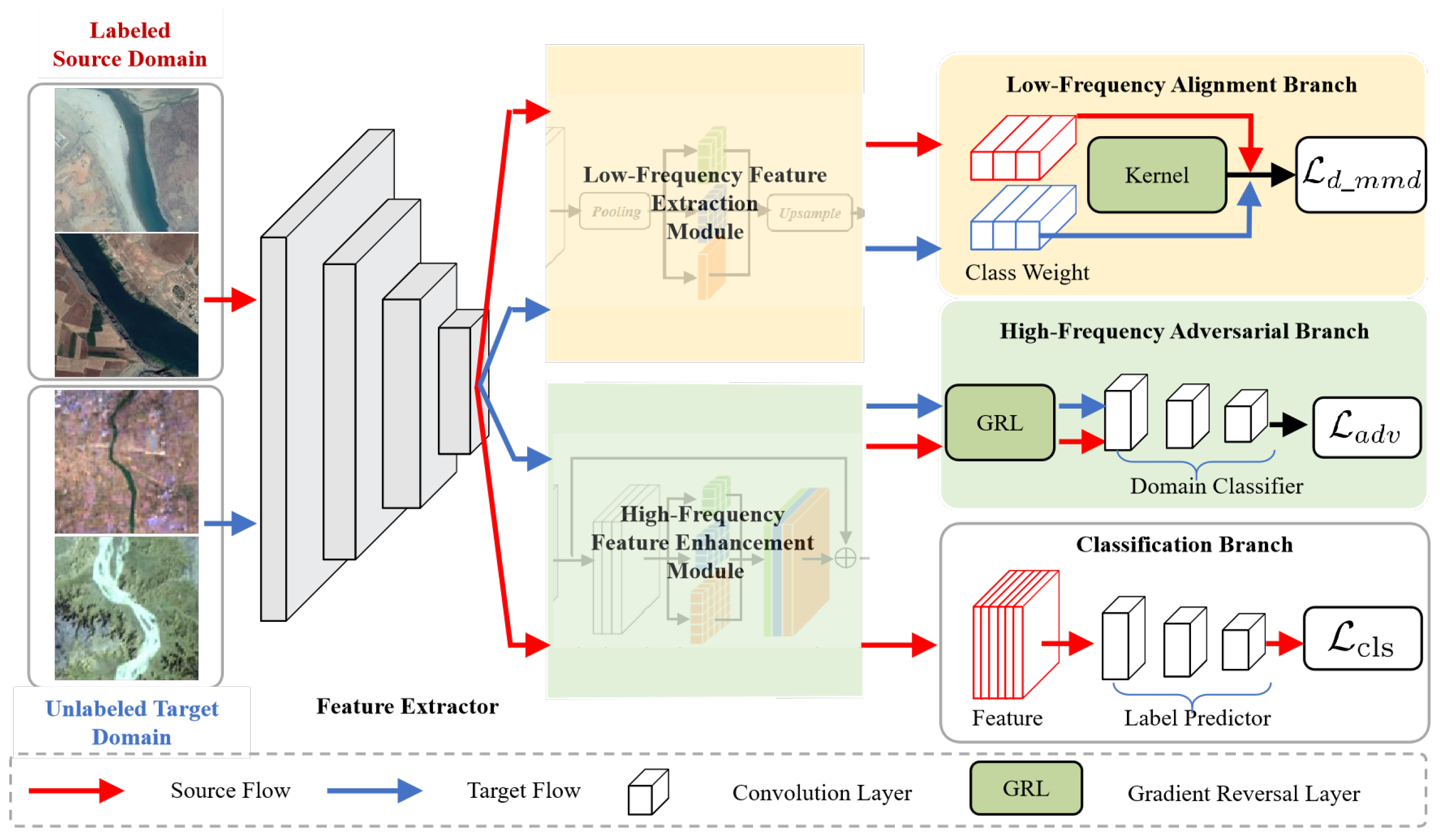
An overview of our proposed method is shown in Figure 2. In the FCAN, the labeled source domain data as well as the unlabeled target domain, respectively, are put through the feature extractor to obtain the initial features. For the high-frequency branch, as shown at the bottom of Figure 2, the high-frequency feature enhancement module (HFE), is first used to enhance the features of the source and target domains, and the high-frequency features of the source domain are supervised with category labeling information. At the same time, the high-frequency features of both the source and target domains are input into the GRL module, which is supervised with domain labeling information. For the low-frequency branch, as shown at the top of Figure 2, the low-frequency features are first extracted using the low-frequency feature extraction module (LFE). Dynamic MMD loss is used for the distribution alignment of the source domain’s low-frequency features and the target domain’s low-frequency features. The red arrows in the figure indicate the labeled source domain data stream and the blue arrows indicate the unlabeled target domain data stream. In the following, we describe the design of the different branches in detail.
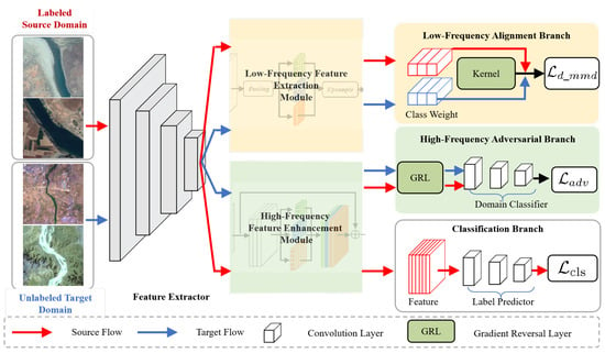
Figure 2.
The proposed FCAN framework. HFE and LFE map the original features into high-frequency components and low-frequency components and adapt them separately, allowing the model to learn more robust domain-invariant features. The high-frequency component features of the source and target domains are constrained using adversarial loss, and the low-frequency component features of the source and target domains are constrained using dynamic maximum mean difference loss.
3.3. High-Frequency Branch
3.3.1. High-Frequency Feature Enhancement Module
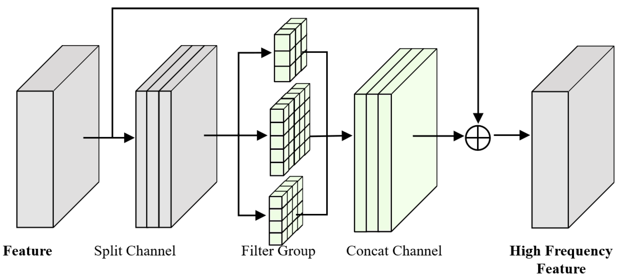
As mentioned earlier, the high-frequency components contain information about the characteristics of the distribution of the data, and utilizing the high-frequency components can boost the CNN’s performance. In order to extract different frequency features, previous work [40] proposed a method based on the Fourier transform and the inverse Fourier transform. However, this approach imposed an additional computational overhead, limiting its use on hardware. We refer to article [41] for a purely convolutional design that avoids the introduction of the Fourier transform. We propose a high-frequency feature enhancement module, and the structure of the HFE module is shown in Figure 3.
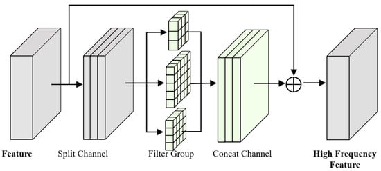
Figure 3.
The proposed HFE module splits the original features in the channel dimension, applies convolutional layers with different kernel sizes for each feature component, and finally concatenates them in the channel dimension.
Considering that each image has a different high-pass cutoff frequency, we perform channel dimensional partitioning of the input features F into n groups to obtain . For each group of features, a convolutional layer with varied kernel sizes is used to mimic the cutoff frequencies of different high-pass filters.
where represents the convolutional layer with kernel size . We splice the resulting sub-features into channel dimensions to obtain enhanced features with the same dimensions as the original input feature space F. Also, to address the problem of vanishing gradients and training difficulties, we introduce a residual structure of shortcut connections. The final high-frequency feature is represented as:
3.3.2. Domain Adversarial Loss
We reduce domain shifting through adversarial learning by introducing a discriminator , which is used to discriminate whether features are from the source or target domains. The discriminator is optimized using cross-entropy of binary classification, as shown in Equation (3).
where q is the domain label , indicating that the feature is from the source or target domain. Adversarial feature alignment is executed by applying a gradient reversal layer (GRL) [30] to the source and target , in which a gradient’s sign is inverted as it is passed through the GRL to optimize the feature extractor. In fact, the GRL, as a kind of optimization solution in the model training process, is essentially the same as the alternating optimization in GANs to achieve the adversarial generation of unbiased representations of the domain. Specifically, in forward propagation, there is , and in back propagation, it has the value , where I is the identity matrix and is a hyperparameter.
We use a dynamic GRL, considering the pre-training period and that the model’s ability to distinguish between different domain data is weak; specifically, the parameter in the GRL is set to gradually increase to ensure a proper balance between competing tasks.
3.4. Classification Branch
We use only labeled source domain data for classification header optimization, and the optimization objective used is the traditional cross-entropy loss.
Here, is the category predictor, is the number of categories in the dataset and is the one-hot encoding of the corresponding label of the image.
3.5. Low-Frequency Branch
3.5.1. Low-Frequency Feature Extraction Filter
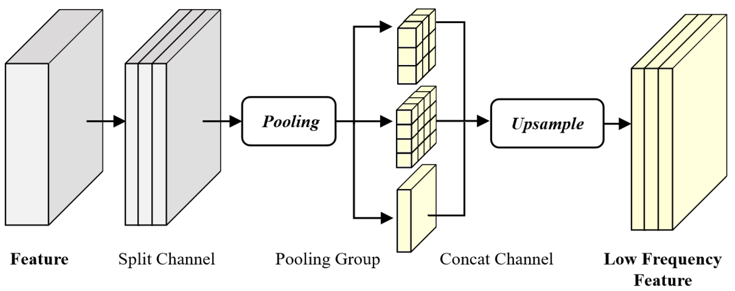
Low-frequency components contain most of the semantic information in an image and are crucial for scene recognition tasks, so we propose a low-frequency feature extraction module (LFE) to capture the low-frequency components in features. For computational convenience, we use the classical average pooling layer as a low-pass filter. Considering that different images have different cutoff frequencies, we refer to the multiscale structure of Inception [42] and expand the single pooling layer, using multiple pooling layers with different kernels, to form a low-pass filter module. In summary, our proposed LFE module is shown in Figure 4.
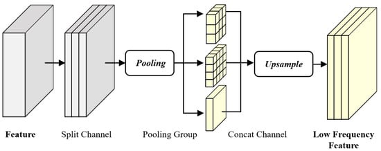
Figure 4.
The proposed LFE module splits the original features in the channel dimension, applies an adaptive pooling layer with different kernel sizes for each feature component, and up-samples them to be consistent with the original feature size, respectively, and then finally concatenates them in the channel dimension.
Considering that each image has a different low-pass cutoff frequency, we perform channel dimensional partitioning of the input features F into m groups to obtain .
where is the bilinear interpolation upsampling layer and is the adaptive average pooling layer with kernel size . After obtaining the low-pass filtering results for the m feature components, we splice them together in the feature dimension to form our final low-frequency feature .
In practice, we set m to 4 and the kernel size to .
3.5.2. DMMD Loss
The low-frequency components of an image, such as information about shape contours, are often directly related to the semantic categories of the image. For remote sensing images obtained under different imaging conditions, we believe that the distribution of their low-frequency components should be as close as possible. LMMD [43] introduces category information on the basis of MMD; i.e., it adds the probability that each sample belongs to each category. We have improved the above losses by imposing a dynamic distributional alignment loss on the low-frequency features of the source domain image and the target domain image.
The weights of the source domain samples are computed from the labels of the source domain samples, and the weights of the target domain samples are computed from the pseudo-labels predicted by the network. In addition, considering the low quality of pseudo-labels at the beginning of training, we introduce dynamic weights .
3.6. Overall Loss
Our model consists of a feature extraction network, a classifier, and a discriminator. The overall optimization objectives include classification loss, adversarial loss for high-frequency components, and alignment loss for low-frequency components. The overall loss formula is:
Among them, the classification loss utilizes the labels in the source domain for supervised learning. The adversarial loss for high-frequency components supervises the high-frequency features in the source and target domains, and the alignment loss for low-frequency components supervises the low-frequency features in the source and target domains. is a weight parameter used to adjust the alignment loss for low-frequency components. In our experiments, we set to 1.0.
4. Experiments
In this section, the two combined datasets for evaluating the effectiveness of the model are first presented, along with the experimental setup. Based on this, a large number of transfer experiments are conducted to validate the effectiveness of the FCAN.
4.1. Description of Cross-Scene Datasets
AID dataset [44]: A large scene classification dataset of remote sensing imagery covering 30 typical scene categories, collected from Google Earth, ranging from 220 to 420 images per category, totaling 10,000 images. Each image is processed to while its pixel resolution is 0.5–8 m.
CLRS dataset [45]: 25 typical scene categories are covered, with 600 images per category, totaling 15,000. Each image is processed to , while its pixel resolution is 0.26–8.85 m.
MLRSN dataset [46]: A large scene classification dataset of remote sensing imagery covering 46 typical scene categories ranging from 1500 to 3000 images for each category, totaling 109,161 images. Each image is processed to while its pixel resolution is 0.1–10 m.
RSSCN7 dataset [47]: Covering seven typical scene categories, captured from Google Earth, each category has 400 remote sensing images, totaling 2800 images. Each image is processed to while its pixel resolution was 0.5–8 m. The dataset is divided into four different scales with 100 images per scale.
We followed [48], and based on the above descriptions of the four remote sensing datasets, we reintegrated the experimental data with the seven public categories of farmland, forest, industry, grassland, parking lot, residential, and river. As a result, the cross-scene dataset has 2500 samples from AID (A), 4200 samples from CLRS (C), 3483 samples from MLRSN (M), and 2800 samples from RSSCN7 (R). We show the combined cross-scene dataset in Figure 5.
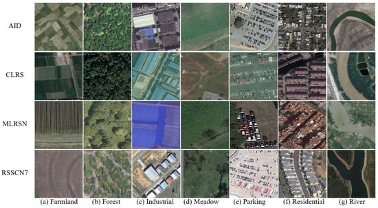
Figure 5.
Sample data from the composite cross-scene dataset used in the experiments. Each column shows the corresponding category for these four datasets, which are farmland, forest, industrial, meadow, parking lot, residential, and river.
4.2. Description of Cross-Sensor Datasets
NWPU-RESISC45 dataset [1]: A large scene classification dataset of remotely sensed imagery covering 45 typical scene categories, collected from Google Earth, with 700 images per category, totaling 31,500 images. Each image is processed to while its pixel resolution is 0.2–30 m.
NaSC-TG2 dataset [49]: It covers 10 typical scene categories, including beach, circular farmland, cloud, desert, forest, mountain range, rectangular farmland, residential area, river and iceberg. Different from other scene classification datasets, this dataset is collected from the imaging spectrometer on board China’s Tiangong-2 space laboratory, totaling 20,000 images. Each image is processed as while its pixel resolution is 100 m.
Based on the above descriptions of the two remote sensing datasets, we take the 10 categories in NaSC-TG2 dataset as the standard, and select the 10 categories common to both in NWPU-RESISC45 as the experimental data. As a result, the composite cross-sensor categorization dataset has 27,000 images, of which NWPU-RESISC45 (N) has a total of 7000 and NaSC-TG2 (T) has 20,000 images. Compared with the composite cross-scene classification dataset, the images in this dataset come from two sensors with large differences in imaging parameters and spectral ranges, and the huge difference in spatial resolution (30 m and 100 m) poses a greater challenge to the cross-domain scene classification algorithm.
4.3. Implementation Details
For all methods compared in the experiments, we use the ResNet-50 model [50] pre-trained on ImageNet [51] as the feature extractor. We use the open-source PyTorch [52] framework for the implementation of all methods, and train and test them on an GeForce RTX 2080Ti GPU equipped with 11 GB of RAM, (Manufactured by ASUS in Taipei, Taiwan). We trained all networks using the SGD optimizer with a batch size of 32 over 20 epochs, with 500 iterations per epoch. The learning rate is initially set to , the momentum is set to 0.9, and the weight decay is set to . Each dataset image was scaled and cropped to a size of 224 × 224 for model training. The data augmentation process employed included random horizontal flipping to improve the generalization performance of the model. Our code is available at https://github.com/MoonExplorer95/FCAN (acessed on 20 May 2024).
We use overall accuracy (OA) as an evaluation criterion for each adaptation task. It is formulated as:
4.4. Baselines
In order to validate the advantages of the FCAN in remote sensing cross-domain scene classification tasks, we compared it with the following methods.
- ERM: The ordinary classification network that trains the model using the labels of the source domain and tests it on the target domain without any adaptation operations. This is our baseline.
- DAN [24] uses MMD loss in CNNs to reduce the distributional difference between source and target domains.
- DANN [30] introduces the idea of adversarial learning for domain confusion.
- DeepCoral [28] uses CORAL losses for distributional difference measures.
- DAAN [53] uses dynamic adversarial factors to regulate the extent to which global distributions and local subdomain distributions contribute to the model and to better learn domain-invariant representations.
- BNM [54] introduces the Batch Nuclear-norm Maximization (BNM) technique for target domain features to improve feature differentiation and diversity.
- DSAN [43] uses the local maximum mean difference to align the distribution of subregions in the source and target domains to facilitate the transfer of domain knowledge.
- AMRAN [13] improves the quality of feature representation using the attention mechanism and aligns the marginal and conditional distributions.
- MRDAN [35] maps samples to multiple representations and fuses them to obtain a broader domain-invariant feature space, adjusting the relative importance of local and global adaptation losses during domain adaptation.
- APA [55] proposes a UDA framework based on penultimate activations for adversarial training to improve the confidence of the model on unlabeled target domain data.
4.5. Comparison with State-of-the-Art Methods
We report the cross-scene classification results in Table 1. Our method achieves the highest average accuracy on the 12 transfer tasks, at 11.5% higher than the baseline ERM method, improving from 74.81% to 86.31%.

Table 1.
Accuracy (%) of a domain adaptation approach in each cross-scene classification task. The best results are bolded.
In terms of individual tasks, the biggest improvement is on the R→M task, with an improvement of 25.87%. The smallest improvement is M→A, which is only improved by 0.92%. As far as the source domain is concerned, using AID, CLRS, MLRSN4 and RSSCN7 as the source domain, the average accuracy improvement is 8.48%, 8.68%, 10.43% and 18.41%, respectively, and RSSCN7 has the largest improvement, which is explained by the fact that RSSCN7 contains four sizes of data, which contain more variations compared to the other three datasets, and the diversity of the sample sizes is more helpful in realizing knowledge transfer. As far as the target domain is concerned, the average accuracy improvement with AID, CLRS, MLRSN and RSSCN7 as the target domain is 6.03%, 12.08%, 14.82% and 13.07%, respectively. AID has the smallest improvement, which is believed to be due to the fact that AID has a single source of data, and also since the sample size of AID is much smaller compared to several other datasets, other data may contain patterns from AID, making transfer easier to achieve.
In comparison with other adaptation methods, we achieve the best performance on the A→C, C→R, M→C, R→A, R→C and R→M tasks. The accuracy of our method is 0.64% higher than the sub-optimal DSAN method.
For the more challenging cross-sensor tasks, as shown in Table 2, our method delivers even greater improvements. We achieved an average accuracy of 94.76% on two tasks. Compared to the baseline method, our method is 32.53% higher. These results on different transfer tasks demonstrate the ability of our method to abbreviate domain gaps and achieve a better classification performance.

Table 2.
Accuracy (%) of a domain adaptation approach in each cross-sensor classification task. The best results are bolded.
4.6. Ablation Study
To further validate our contribution, we performed ablation experiments on the cross-scene dataset.
Effectiveness of Each Module. Our FCAN model is divided into a high-frequency branch and a low-frequency branch, and the overall objective function consists of three components: a supervised classification loss for source domain data, a domain classification loss for improving domain discrimination, and a distributional difference metric loss for aligning low-frequency features. In order to investigate the effectiveness of different module designs in our proposed FCAN, ResNet-50 is adopted as the backbone of the CNN; we perform FCAN ablation experiments on all 12 adaptation tasks on a cross-scene dataset. Table 3 reports the experimental results.

Table 3.
Ablation experiment results on each module of the FCAN. ✔ and ✘ represent the use and non-use of the component, respectively.
When using only the supervised classification loss , which is the ERM algorithm, only a 74.81% average classification accuracy is obtained across all 12 adaptation tasks. After the introduction of the adversarial learning strategy, also known as the classical DANN algorithm, the average classification accuracy significantly improved to 83.46%. Similarly, with the introduction of MMD loss, which is the classical DAN algorithm, on top of ERM, the average classification accuracy was improved to 81.03%, indicating that both the adversarial learning strategy and the distributional difference metric strategy are able to confuse the distributions of the source and target domains effectively, also proving that the domain adaptation method based on the adversarial learning strategy is more advantageous than the one based on the distributional difference metric strategy.
By embedding our proposed high-frequency feature enhancement module into the DANN framework, the average accuracy is further improved to 83.90%, which indicates that the high-frequency features have a better generalization performance than the original features. After the introduction of the low-frequency feature branch, the average accuracy of classification is improved to 84.31% using the original MMD alignment loss, which indicates that aligning the low-frequency features can further bridge the distributional differences between the source and target domains. After replacing the original MMD loss with DMMD loss, the average classification accuracy finally reaches 86.31%, which is 11.5% higher than the baseline of ERM, 2.85% higher than the pure adversarial learning method, and 5.28% higher than the pure distributional discrepancy metric alignment method.
Figure 6 shows the confusion matrix of the three methods of ERM, ERM with the introduction of high-frequency feature-enhanced branching, and the full FCAN on the R→A task. It can be observed that the diagonal elements of the confusion matrix are gradually concentrated and deepen in color, which further validates the effectiveness of our algorithm. For the categories “Farmland” and “Meadow”, which are visually very similar, ERM has difficulty distinguishing between these two categories. Our high-frequency feature branch can effectively reduce the confusion between the two categories and achieve more accurate cross-scene classification.

Figure 6.
The confusion matrices of the methods of ERM, ERM+HFE, and the proposed FCAN in the R→A adaptation task.
Parameter sensitivity analysis. is a hyperparameter used to regulate the degree of contribution of low-frequency alignment loss. We analyzed five values of {0.0, 0.25, 0.50, 0.75, 1.0}. The final results on the 12 tasks are shown in Figure 7. The red dashed line represents the mean value for each task. When is equal to 1.0, the best results can be achieved on the three source domain tasks, AID, CLRS and RSSCN7. When is equal to 0.5, the best results can be achieved on the source domain task of MLRSN.
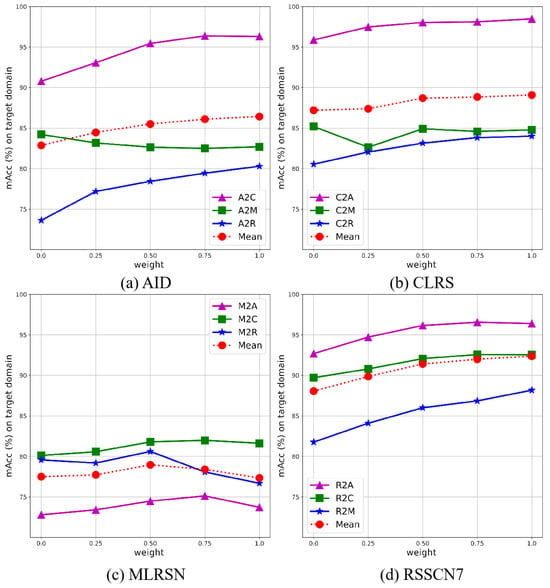
Figure 7.
Classification accuracy of the proposed FCAN with different weights for the low-frequency feature alignment loss.
Efficiency and Complexity. To evaluate the operational efficiency, we compare the training time of different methods. The criterion is the average time spent per iteration for different models. For a fair comparison, we set the batchsize to 32 uniformly and performed an efficiency evaluation of various methods on GeForce GTX 2080 Ti GPUs, (manufactured by ASUS in Taipei, Taiwan). The results are shown in the rightmost column of Table 4. ERM without the domain adaptation module and the APA model with direct fine-tuning took the least amount of time. Our model requires the same amount of time as most of the methods that incorporate the domain adaptation module. To assess the complexity, we compared the computational complexity and the number of parameters of the different methods. Since the low-frequency and high-frequency modules used in our method are lightweight, they do not add too many model parameters. The introduction of multiple cutoff frequencies, on the other hand, caused a rise in computational overhead. However, it is worthwhile adding a small amount of computational resources to further improve the performance.

Table 4.
Model efficiency and complexity comparison.
Distribution Discrepancy. We also analyze the ability of different models to reduce the domain gap. -Distance [56] is a metric that estimates the variability between different distributions. It is calculated as , which additionally defines a classifier for binary classification of source and target domain data, and is the generalization error of this classifier. Specifically, after training the model, we obtain the source domain features and the target domain features and then use them as samples to train a single-layer linear classifier, and the classification error rate is taken as . A large means a large generalization error. Figure 8 shows the -Distance results of the four methods, ERM, DAN, DANN and FCAN, on the four tasks. As can be seen, our proposed FCAN method has the smallest a-distance on multiple tasks, which means that FCAN is more capable of bridging domain differences compared to other methods.
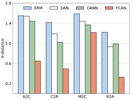
Figure 8.
Results of the a-distance of the proposed FCAN on four different transfer learning tasks.
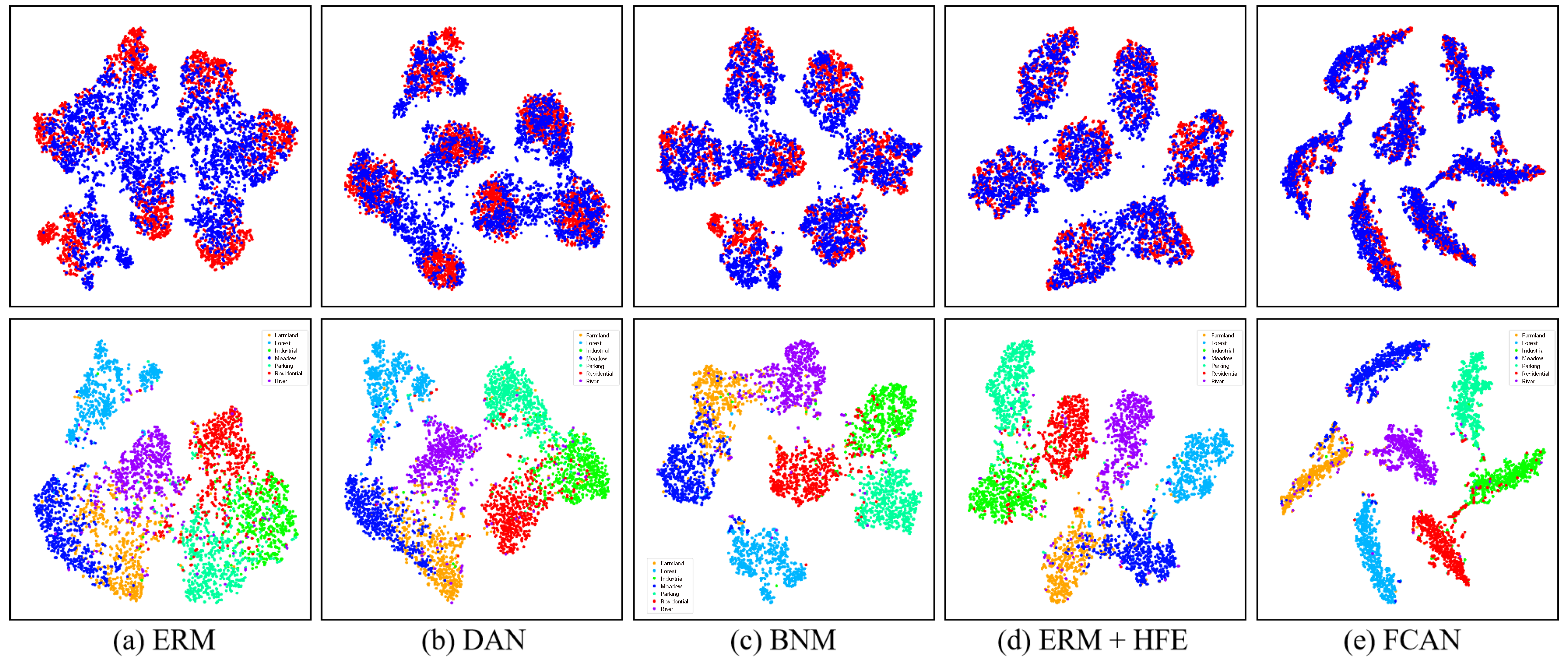
Visualization of feature distribution. To further demonstrate the effectiveness of the FCAN, we visualize the features learned by different models before the classifiers using the T-SNE method [57] for the task R→C. These comparisons include longitudinal comparison methods such as DAN and BNM, as well as horizontal comparison methods such as ERM, the ERM with added high-frequency branches, and our full FCAN. Notably, we performed two different feature visualization comparisons, as shown in Figure 9, where the first row shows domain-wise comparisons, with blue scatters representing the features of the source domain samples and red scatters representing the features of the target domain samples. This assesses the generalization ability of different methods. The second row shows class-wise comparisons, with different colors representing the features of different classes of samples. This assesses the discriminative ability of different methods.
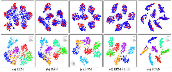
Figure 9.
The t-SNE visualization plots of the feature distributions of the FCAN and other methods in an R→C adaptation task.
As shown in Figure 9a–c, the distribution of features in the target domain and the distribution of features in the source domain are more variable in methods such as ERM, and there is more overlap between the clusters of features of different sample classes in the target domain. As shown in Figure 9d, the difference between the target domain feature distributions and source domain feature distributions is further reduced after the addition of high-frequency branches. As shown in Figure 9e, after adding the dynamic maximum mean difference constraint, our proposed FCAN maps the sample features into a shuttle shape, which is different from the circular region of other methods and separates the features of different sample categories to a greater extent.
As shown in Figure 10, we further visualize the spectrum of the features of different branches. Compared with ERM, the spectrogram energy of the low-frequency branch is more concentrated in the center, indicating that the low-frequency module is indeed able to extract low-frequency information from the image. The energy of the spectrograms of the high-frequency branch is dispersed in the four corners, indicating that the high-frequency module can indeed extract high-frequency information from the image. The above results show that our method can meet the aims of this article.

Figure 10.
Fourier spectrum of ERM, HFE and LFE.
5. Conclusions
A method based on frequency component decomposition is designed for the remote sensing cross-domain scene classification problem. This method includes two adaptation mechanisms: alignment of low-frequency features and adversarial training of high-frequency features. Using a high-frequency feature enhancement module and a low-frequency feature extraction module, the original features are mapped into high-frequency features and low-frequency features. Then, adversarial constraints are applied to the high-frequency features in the source and target domains, and dynamic maximum mean difference constraints are applied to the low-frequency features in the source and target domains, which together enhance the generalization of the model. The experimental results demonstrate the ability of this method to improve the performance in the transfer task. In future work, we will carry out research on the source-free adaptation task, considering the storage cost and privacy issues of source-domain samples.
Author Contributions
Conceptualization, X.Z. and P.Z.; funding acquisition, X.Z. and J.G.; methodology, P.Z., X.Z. and X.H.; software, P.Z., J.G. and P.C.; supervision, X.Z., P.Z. and L.J.; writing—original draft, P.Z.; writing—review and editing, X.Z., X.C. and P.C. All authors have read and agreed to the published version of the manuscript.
Funding
This work was supported in part by the National Natural Science Foundation of China under Grant 62276197, Grant 62006178, and Grant 62171332, and in part by the Key Research and Development Program in the Shaanxi Province Innovation Capability Support Plan under Grant 2023-CX-TD-09.
Data Availability Statement
AID, CLRS, MLRSN, RSSCN7, NWPU-RESISC45, and NaSC-TG2 can be found at: https://captain-whu.github.io/AID/, https://github.com/lehaifeng/CLRS, https://github.com/cugbrs/MLRSNet, https://github.com/palewithout/RSSCN7, http://pan.baidu.com/s/1mifR6tU, https://captain-whu.github.io/BED4RS/ accessed on 1 May 2024.
Conflicts of Interest
The authors declare no conflicts of interest.
Abbreviations
The following abbreviations are used in this manuscript:
| DA | Domain Adaptation |
| HFE | High-frequency Feature Enhancement Module |
| LFE | Low-frequency Feature Extraction Module |
| FCAN | Frequency Component Adaptation Network |
| GRL | Gradient Reversal Layer |
| MMD | Maximum Mean Discrepancy |
| OA | Overall Accuracy |
References
- Cheng, G.; Li, Z.; Yao, X.; Guo, L.; Wei, Z. Remote sensing image scene classification using bag of convolutional features. IEEE Geosci. Remote Sens. Lett. 2017, 14, 1735–1739. [Google Scholar] [CrossRef]
- Wang, Q.; Liu, S.; Chanussot, J.; Li, X. Scene classification with recurrent attention of VHR remote sensing images. IEEE Trans. Geosci. Remote Sens. 2018, 57, 1155–1167. [Google Scholar] [CrossRef]
- Lu, X.; Sun, H.; Zheng, X. A feature aggregation convolutional neural network for remote sensing scene classification. IEEE Trans. Geosci. Remote Sens. 2019, 57, 7894–7906. [Google Scholar] [CrossRef]
- Cheng, G.; Xie, X.; Han, J.; Guo, L.; Xia, G.S. Remote sensing image scene classification meets deep learning: Challenges, methods, benchmarks, and opportunities. IEEE J. Sel. Top. Appl. Earth Obs. Remote Sens. 2020, 13, 3735–3756. [Google Scholar] [CrossRef]
- Ma, L.; Li, M.; Ma, X.; Cheng, L.; Du, P.; Liu, Y. A review of supervised object-based land-cover image classification. ISPRS J. Photogramm. Remote Sens. 2017, 130, 277–293. [Google Scholar] [CrossRef]
- Ma, L.; Liu, Y.; Zhang, X.; Ye, Y.; Yin, G.; Johnson, B.A. Deep learning in remote sensing applications: A meta-analysis and review. ISPRS J. Photogramm. Remote Sens. 2019, 152, 166–177. [Google Scholar] [CrossRef]
- Cheng, G.; Yang, C.; Yao, X.; Guo, L.; Han, J. When deep learning meets metric learning: Remote sensing image scene classification via learning discriminative CNNs. IEEE Trans. Geosci. Remote Sens. 2018, 56, 2811–2821. [Google Scholar] [CrossRef]
- Xie, J.; He, N.; Fang, L.; Plaza, A. Scale-free convolutional neural network for remote sensing scene classification. IEEE Trans. Geosci. Remote Sens. 2019, 57, 6916–6928. [Google Scholar] [CrossRef]
- Xu, M.; Wu, M.; Chen, K.; Zhang, C.; Guo, J. The eyes of the gods: A survey of unsupervised domain adaptation methods based on remote sensing data. Remote Sens. 2022, 14, 4380. [Google Scholar] [CrossRef]
- Peng, J.; Huang, Y.; Sun, W.; Chen, N.; Ning, Y.; Du, Q. Domain adaptation in remote sensing image classification: A survey. IEEE J. Sel. Top. Appl. Earth Obs. Remote Sens. 2022, 15, 9842–9859. [Google Scholar] [CrossRef]
- Tong, X.Y.; Xia, G.S.; Lu, Q.; Shen, H.; Li, S.; You, S.; Zhang, L. Land-cover classification with high-resolution remote sensing images using transferable deep models. Remote Sens. Environ. 2020, 237, 111322. [Google Scholar] [CrossRef]
- Othman, E.; Bazi, Y.; Melgani, F.; Alhichri, H.; Alajlan, N.; Zuair, M. Domain adaptation network for cross-scene classification. IEEE Trans. Geosci. Remote Sens. 2017, 55, 4441–4456. [Google Scholar] [CrossRef]
- Zhu, S.; Du, B.; Zhang, L.; Li, X. Attention-based multiscale residual adaptation network for cross-scene classification. IEEE Trans. Geosci. Remote Sens. 2021, 60, 5400715. [Google Scholar] [CrossRef]
- Yang, C.; Dong, Y.; Du, B.; Zhang, L. Attention-based dynamic alignment and dynamic distribution adaptation for remote sensing cross-domain scene classification. IEEE Trans. Geosci. Remote Sens. 2022, 60, 5634713. [Google Scholar] [CrossRef]
- Wei, H.; Ma, L.; Liu, Y.; Du, Q. Combining multiple classifiers for domain adaptation of remote sensing image classification. IEEE J. Sel. Top. Appl. Earth Obs. Remote Sens. 2021, 14, 1832–1847. [Google Scholar] [CrossRef]
- Zhang, J.; Liu, J.; Pan, B.; Shi, Z. Domain adaptation based on correlation subspace dynamic distribution alignment for remote sensing image scene classification. IEEE Trans. Geosci. Remote Sens. 2020, 58, 7920–7930. [Google Scholar] [CrossRef]
- Yan, L.; Zhu, R.; Mo, N.; Liu, Y. Cross-domain distance metric learning framework with limited target samples for scene classification of aerial images. IEEE Trans. Geosci. Remote Sens. 2019, 57, 3840–3857. [Google Scholar] [CrossRef]
- Teng, W.; Wang, N.; Shi, H.; Liu, Y.; Wang, J. Classifier-constrained deep adversarial domain adaptation for cross-domain semisupervised classification in remote sensing images. IEEE Geosci. Remote Sens. Lett. 2019, 17, 789–793. [Google Scholar] [CrossRef]
- Zhu, S.; Wu, C.; Du, B.; Zhang, L. Adversarial Divergence Training for Universal Cross-scene Classification. IEEE Trans. Geosci. Remote Sens. 2023. [Google Scholar] [CrossRef]
- Zheng, Z.; Zhong, Y.; Su, Y.; Ma, A. Domain adaptation via a task-specific classifier framework for remote sensing cross-scene classification. IEEE Trans. Geosci. Remote Sens. 2022, 60, 5620513. [Google Scholar] [CrossRef]
- Zhang, X.; Yao, X.; Feng, X.; Cheng, G.; Han, J. DFENet for domain adaptation-based remote sensing scene classification. IEEE Trans. Geosci. Remote Sens. 2021, 60, 5611611. [Google Scholar] [CrossRef]
- Wang, H.; Wu, X.; Huang, Z.; Xing, E.P. High-frequency component helps explain the generalization of convolutional neural networks. In Proceedings of the IEEE/CVF Conference on Computer Vision and Pattern Recognition, Seattle, WA, USA, 14–19 June 2020; pp. 8684–8694. [Google Scholar]
- Wang, M.; Deng, W. Deep visual domain adaptation: A survey. Neurocomputing 2018, 312, 135–153. [Google Scholar] [CrossRef]
- Tzeng, E.; Hoffman, J.; Zhang, N.; Saenko, K.; Darrell, T. Deep domain confusion: Maximizing for domain invariance. arXiv 2014, arXiv:1412.3474. [Google Scholar]
- Long, M.; Cao, Y.; Wang, J.; Jordan, M. Learning transferable features with deep adaptation networks. In Proceedings of the International Conference on Machine Learning, Lille, France, 7–9 July 2015; pp. 97–105. [Google Scholar]
- Long, M.; Zhu, H.; Wang, J.; Jordan, M.I. Deep transfer learning with joint adaptation networks. In Proceedings of the International Conference on Machine Learning, Sydney, Australia, 6–11 August 2017; pp. 2208–2217. [Google Scholar]
- Yan, H.; Ding, Y.; Li, P.; Wang, Q.; Xu, Y.; Zuo, W. Mind the class weight bias: Weighted maximum mean discrepancy for unsupervised domain adaptation. In Proceedings of the IEEE Conference on Computer Vision and Pattern Recognition, Honolulu, HI, USA, 21–26 July 2017; pp. 2272–2281. [Google Scholar]
- Sun, B.; Saenko, K. Deep coral: Correlation alignment for deep domain adaptation. In Proceedings of the Computer Vision–ECCV 2016 Workshops, Amsterdam, The Netherlands, 8–10 October 2016; Proceedings, Part III 14. Springer: Berlin/Heidelberg, Germany, 2016; pp. 443–450. [Google Scholar]
- Goodfellow, I.; Pouget-Abadie, J.; Mirza, M.; Xu, B.; Warde-Farley, D.; Ozair, S.; Courville, A.; Bengio, Y. Generative adversarial nets. Adv. Neural Inf. Process. Syst. 2014, 27, 139–144. [Google Scholar] [CrossRef]
- Ganin, Y.; Lempitsky, V. Unsupervised domain adaptation by backpropagation. In Proceedings of the International Conference on Machine Learning, Lille, France, 7–9 July 2015; pp. 1180–1189. [Google Scholar]
- Long, M.; Cao, Z.; Wang, J.; Jordan, M.I. Conditional adversarial domain adaptation. Adv. Neural Inf. Process. Syst. 2018, 31, 1647–1657. [Google Scholar]
- Tao, C.; Xiao, R.; Wang, Y.; Qi, J.; Li, H. A General Transitive Transfer Learning Framework for Cross-Optical Sensor Remote Sensing Image Scene Understanding. IEEE J. Sel. Top. Appl. Earth Obs. Remote Sens. 2023, 16, 4248–4260. [Google Scholar] [CrossRef]
- Zhao, Y.; Li, S.; Liu, C.H.; Han, Y.; Shi, H.; Li, W. Domain adaptive remote sensing scene recognition via semantic relationship knowledge transfer. IEEE Trans. Geosci. Remote Sens. 2023, 61, 2001013. [Google Scholar] [CrossRef]
- Huang, W.; Shi, Y.; Xiong, Z.; Wang, Q.; Zhu, X.X. Semi-supervised bidirectional alignment for remote sensing cross-domain scene classification. ISPRS J. Photogramm. Remote Sens. 2023, 195, 192–203. [Google Scholar] [CrossRef]
- Niu, B.; Pan, Z.; Wu, J.; Hu, Y.; Lei, B. Multi-representation dynamic adaptation network for remote sensing scene classification. IEEE Trans. Geosci. Remote Sens. 2022, 60, 5633119. [Google Scholar] [CrossRef]
- Dong, Y.; Qin, X.; Li, X.; Xu, L. Multilevel Spatial Features-Based Manifold Metric Learning for Domain Adaptation in Remote Sensing Image Classification. IEEE Trans. Geosci. Remote Sens. 2023, 61, 5527414. [Google Scholar] [CrossRef]
- Chen, Y.; Teng, W.; Li, Z.; Zhu, Q.; Guan, Q. Cross-domain scene classification based on a spatial generalized neural architecture search for high spatial resolution remote sensing images. Remote Sens. 2021, 13, 3460. [Google Scholar] [CrossRef]
- Xu, C.; Shu, J.; Zhu, G. Multi-Feature Dynamic Fusion Cross-Domain Scene Classification Model Based on Lie Group Space. Remote Sens. 2023, 15, 4790. [Google Scholar] [CrossRef]
- Zhang, X.; Zhuang, Y.; Zhang, T.; Li, C.; Chen, H. Masked Image Modeling Auxiliary Pseudo-Label Propagation with a Clustering Central Rectification Strategy for Cross-Scene Classification. Remote Sens. 2024, 16, 1983. [Google Scholar] [CrossRef]
- Rao, Y.; Zhao, W.; Zhu, Z.; Lu, J.; Zhou, J. Global filter networks for image classification. Adv. Neural Inf. Process. Syst. 2021, 34, 980–993. [Google Scholar]
- Dong, B.; Wang, P.; Wang, F. Head-free lightweight semantic segmentation with linear transformer. In Proceedings of the AAAI Conference on Artificial Intelligence, Washiongton, DC, USA, 7–14 February 2023; Volume 37, pp. 516–524. [Google Scholar]
- Szegedy, C.; Vanhoucke, V.; Ioffe, S.; Shlens, J.; Wojna, Z. Rethinking the inception architecture for computer vision. In Proceedings of the IEEE Conference on Computer Vision and Pattern Recognition, Las Vegas, NV, USA, 27–30 June 2016; pp. 2818–2826. [Google Scholar]
- Zhu, Y.; Zhuang, F.; Wang, J.; Ke, G.; Chen, J.; Bian, J.; Xiong, H.; He, Q. Deep subdomain adaptation network for image classification. IEEE Trans. Neural Netw. Learn. Syst. 2020, 32, 1713–1722. [Google Scholar] [CrossRef] [PubMed]
- Xia, G.S.; Hu, J.; Hu, F.; Shi, B.; Bai, X.; Zhong, Y.; Zhang, L.; Lu, X. AID: A benchmark data set for performance evaluation of aerial scene classification. IEEE Trans. Geosci. Remote Sens. 2017, 55, 3965–3981. [Google Scholar] [CrossRef]
- Li, H.; Jiang, H.; Gu, X.; Peng, J.; Li, W.; Hong, L.; Tao, C. CLRS: Continual learning benchmark for remote sensing image scene classification. Sensors 2020, 20, 1226. [Google Scholar] [CrossRef] [PubMed]
- Qi, X.; Zhu, P.; Wang, Y.; Zhang, L.; Peng, J.; Wu, M.; Chen, J.; Zhao, X.; Zang, N.; Mathiopoulos, P.T. MLRSNet: A multi-label high spatial resolution remote sensing dataset for semantic scene understanding. ISPRS J. Photogramm. Remote Sens. 2020, 169, 337–350. [Google Scholar] [CrossRef]
- Zou, Q.; Ni, L.; Zhang, T.; Wang, Q. Deep learning based feature selection for remote sensing scene classification. IEEE Geosci. Remote Sens. Lett. 2015, 12, 2321–2325. [Google Scholar] [CrossRef]
- Zhu, S.; Wu, C.; Du, B.; Zhang, L. Style and content separation network for remote sensing image cross-scene generalization. ISPRS J. Photogramm. Remote Sens. 2023, 201, 1–11. [Google Scholar] [CrossRef]
- Zhou, Z.; Li, S.; Wu, W.; Guo, W.; Li, X.; Xia, G.; Zhao, Z. NaSC-TG2: Natural scene classification with Tiangong-2 remotely sensed imagery. IEEE J. Sel. Top. Appl. Earth Obs. Remote Sens. 2021, 14, 3228–3242. [Google Scholar] [CrossRef]
- He, K.; Zhang, X.; Ren, S.; Sun, J. Deep residual learning for image recognition. In Proceedings of the IEEE Conference on Computer Vision and Pattern Recognition, Las Vegas, NV, USA, 26 June–1 July 2016; pp. 770–778. [Google Scholar]
- Deng, J.; Dong, W.; Socher, R.; Li, L.J.; Li, K.; Fei-Fei, L. Imagenet: A large-scale hierarchical image database. In Proceedings of the 2009 IEEE Conference on Computer Vision and Pattern Recognition, Miami, FL, USA, 20–25 June 2009; pp. 248–255. [Google Scholar]
- Paszke, A.; Gross, S.; Massa, F.; Lerer, A.; Bradbury, J.; Chanan, G.; Killeen, T.; Lin, Z.; Gimelshein, N.; Antiga, L.; et al. Pytorch: An imperative style, high-performance deep learning library. Adv. Neural Inf. Process. Syst. 2019, 32, 8026–8037. [Google Scholar]
- Yu, C.; Wang, J.; Chen, Y.; Huang, M. Transfer learning with dynamic adversarial adaptation network. In Proceedings of the 2019 IEEE International Conference on Data Mining (ICDM), Beijing, China, 8–11 November 2019; pp. 778–786. [Google Scholar]
- Cui, S.; Wang, S.; Zhuo, J.; Li, L.; Huang, Q.; Tian, Q. Towards discriminability and diversity: Batch nuclear-norm maximization under label insufficient situations. In Proceedings of the IEEE/CVF Conference on Computer Vision and Pattern Recognition, Seattle, WA, USA, 13–19 June 2020; pp. 3941–3950. [Google Scholar]
- Sun, T.; Lu, C.; Ling, H. Domain adaptation with adversarial training on penultimate activations. In Proceedings of the AAAI Conference on Artificial Intelligence, Washington, DC, USA, 7–14 February 2023; Volume 37, pp. 9935–9943. [Google Scholar]
- Ben-David, S.; Blitzer, J.; Crammer, K.; Kulesza, A.; Pereira, F.; Vaughan, J.W. A theory of learning from different domains. Mach. Learn. 2010, 79, 151–175. [Google Scholar] [CrossRef]
- Van der Maaten, L.; Hinton, G. Visualizing data using t-SNE. J. Mach. Learn. Res. 2008, 9, 2579–2605. [Google Scholar]
Disclaimer/Publisher’s Note: The statements, opinions and data contained in all publications are solely those of the individual author(s) and contributor(s) and not of MDPI and/or the editor(s). MDPI and/or the editor(s) disclaim responsibility for any injury to people or property resulting from any ideas, methods, instructions or products referred to in the content. |
© 2024 by the authors. Licensee MDPI, Basel, Switzerland. This article is an open access article distributed under the terms and conditions of the Creative Commons Attribution (CC BY) license (https://creativecommons.org/licenses/by/4.0/).

