Technical Note

Integration of Handheld and Airborne Lidar Data for Dicranopteris Dichotoma Biomass Estimation in a Subtropical Region of Fujian Province, China

1
Institute of Geography, Fujian Normal University, Fuzhou 350117, China
2
Key Laboratory for Humid Subtropical Eco-Geographical Processes of the Ministry of Education, Fujian Normal University, Fuzhou 350117, China
3
Fujian Soil and Water Conservation Experimental Station, Fuzhou 350003, China
*
Author to whom correspondence should be addressed.
Remote Sens. 2024, 16(12), 2088; https://doi.org/10.3390/rs16122088
Submission received: 21 April 2024 / Revised: 1 June 2024 / Accepted: 6 June 2024 / Published: 9 June 2024

Abstract

:
Dicranopteris dichotoma is a pioneer herbaceous plant species that is tolerant to barrenness and drought. Mapping its biomass spatial distribution is valuable for understanding its important role in reducing soil erosion and restoring ecosystems. This research selected Luodihe watershed in Changting County, Fujian Province, China, where soil erosion has been a severe problem for a long time, as a case study to explore the method to estimate biomass, including total and aboveground biomass, through the integration of field measurements, handheld laser scanning (HLS), and airborne laser scanning (ALS) data. A stepwise regression model and an allometric equation form model were used to develop biomass estimation models based on Lidar-derived variables at typical areas and at a regional scale. The results indicate that at typical areas, both total and aboveground biomass were best estimated using an allometric equation form model when HLS-derived height and density variables were extracted from a window size of 6 m × 6 m, with the coefficients of determination (R2) of 0.64 and 0.58 and relative root mean square error (rRMSE) of 28.2% and 35.8%, respectively. When connecting HLS-estimated biomass with ALS-derived variables at a regional scale, total and aboveground biomass were effectively predicted with rRMSE values of 17.68% and 17.91%, respectively. The HLS data played an important role in linking field measurements and ALS data. This research provides a valuable method to map Dicranopteris biomass distribution using ALS data when other remotely sensed data cannot effectively estimate the understory vegetation biomass. The estimated biomass spatial pattern will be helpful to understand the role of Dicranopteris in reducing soil erosion and improving the degraded ecosystem.

1. Introduction

Dicranopteris dichotoma is a type of fern that is extensively distributed in red-soil hills or under Masson pine forests in subtropical regions [1,2,3]. It is a pioneer herbaceous species that can grow in poor site conditions, with a strong survival ability in infertile soils, forming a dominant plant community for the restoration of degraded ecosystems due to severe soil erosion in subtropical regions [4]. The Dicranopteris roots can stabilize the soil structure and provide necessary habitat and nutrient sources for belowground microbes [5]. Thus, Dicranopteris plays an important role in carbon fixation, soil moisture regulation, nutrient cycling [5,6], and in maintaining biodiversity and ecosystem sustainability [7,8]. Therefore, mapping the spatial distribution of Dicranopteris biomass is valuable for assessing the effectiveness of implementing conservation measures on the restoration of degraded ecosystems.
Traditional studies related to Dicranopteris are often focused on the nutrient cycling, photosynthesis, and improvement in soil characteristics, which are relevant to the biological structures and functions and physical–chemical properties [9,10,11,12]. The biomass-related studies are mainly based on field measurements, which is based on leaf spread size and height for aboveground biomass, or uses rhizome length to establish the root biomass estimation model [2]. These methods are only suitable for plot level because of the labor intensity and cost, and cannot provide spatial distribution of Dicranopteris biomass. Another way to calculate Dicranopteris biomass is through plot survey, that is, harvesting and measuring the aboveground fern biomass and belowground roots. This method can accurately collect biomass that is required for establishing the allometric equations based on coverage and/or height. However, collection of sufficient plot data is a challenge because of the difficulty and cost of field surveys.
The advance in remote sensing technologies makes it possible to estimate biomass in a large area [13]. In the past four decades, many studies have been conducted to map forest or grass biomass at different scales using optical sensor or SAR data [13,14]. However, the signal saturation and radiometric data uncertainty caused by external environmental conditions resulted in poor biomass estimation using optical or SAR data alone [15,16]. Because optical or SAR data mainly capture the canopy surface features, it is difficult to use them to estimate understory biomass. The Lidar technology, due to its ability in accurately capturing three-dimensional forest stand features, becomes an important data source for biomass estimation [17], especially for the understory vegetation.
Lidar data can be obtained by Lidar systems that are mounted on different platforms such as ground, aircraft, and satellite. In the application of forestry, ground-based instruments, including terrestrial-, handheld-, and backpack-laser scanning devices, are often used for collection of point clouds at small areas, capturing three-dimensional forest stand structure, particularly vegetation of lower layers [18,19,20]. Thus, they are often used to extract individual tree parameters such as diameter at breast height (DBH), tree height, and crown size. Other common Lidar data sources are airborne Lidar, especially the unmanned aerial vehicle (UAV), which obtain high density of point clouds valuable for extraction of tree or canopy height in a relatively large area [17]. To take advantages of terrestrial laser scanning (TLS) and UAV Lidar data, Panagiotidis et al. [21] fused them together and improved extraction accuracies of tree metrics, such as DBH, tree height, crown projection area, crown width/length, 3D crown surface, and 3D crown volume.
In recent years, many studies have been conducted to accurately estimate forest biomass, mostly aboveground biomass in different climate regions [22], but the estimation of understory vegetation biomass using Lidar data has rarely been examined. The possible reasons may be the lack of ground truth data and the small proportion accounting for total biomass. However, the important role of understory vegetation in reducing soil erosion problems and in improving ecosystem functions make it valuable for accurately mapping the spatial distribution of Dicranopteris biomass.
While aboveground biomass (AGB) can be directly related to the variables derived from remote sensing data (Lidar data in this study) and modeled using different algorithms, the belowground biomass (BGB) estimation based on remote sensing techniques is much less common than aboveground biomass because BGB cannot be readily observed by satellites or airborne sensors [23,24]. Moreover, BGB samples are difficult to measure and collect, and models are hard to develop and validate. Therefore, BGB is often inferred using region-, climate-, or vegetation-specific ‘root-to-shoot ratio’. In recent years, more advanced methods have been developed to predict ‘root-to-shoot ratio’ for land covers, and vegetation types [25,26,27]. Particularly, Ma et al. [27] created a database of ‘root-mass fractions’, an index of plant BGB vs. AGB and generated global maps of ‘root-mass fractions’ in trees, shrubs, and grasses, which can be used to estimate BGB based on existing global or regional AGB maps.
Handheld laser scanning (HLS) devices can capture understory vegetation features through bottom-up scanning way, but are mainly suitable at plot level due to large data volume and field operation, while airborne laser scanning (ALS) devices can provide three-dimensional forest features in a relatively large area through top-down scanning but it is difficult to obtain detailed understory vegetation features. In the light of the complementary merits of HLS and ALS, how to make full use of their advantages for accurate estimation of Dicranopteris biomass is poorly understood. This research selects Luodihe watershed in Changting County, Fujian Province, China as a case study to explore the potential of using field measurements, and HLS and ALS data to estimate Dicranopteris aboveground and total biomass, respectively. This research is valuable for applying proper Lidar data to the accurate estimation of grass biomass in a large area. The results will be helpful for local government to make scientific decisions for improving the degraded ecosystem due to soil erosion problems.

2. Study Area

The study area is located in the southwestern part of Fujian Province, once one of the regions most afflicted by severe soil and water erosion in China, but is now an example for its success in water and soil erosion control. This research selected the Luodihe watershed (see Figure 1), a typical area of implementing conservation measures during the past three decades, as a case study to explore the possible methods to estimate understory biomass using Lidar data. This watershed has an area of 26.23 km2 with relatively complex topographic conditions, which are mainly composed of hills and low mountains with elevation of less than 630 m. The region belongs to a central subtropical monsoon humid climate with warm and humid spring and summer seasons and cold and dry fall and winter seasons. The annual average temperature is 18.8 °C and the annual average precipitation is 1700 mm, with high annual variation. The rainfall is mainly in April–June, accounting for 51.8%, and in July–September, the typhoon season [8]. The dominant soil type is red soil with strong acidity, a thin soil layer, poor capability of preserving water and nutrients, and weak soil erosion resistance, resulting in severe water and soil erosion. Because of long-term severe soil erosion, an original evergreen broadleaf forest did not exist, and instead is currently dominated by Masson pine with simple tree species and stand structure [28]. Because of the poor soil fertility conditions, Dicranopteris dichotoma is the dominant vegetation under pine forests due to both species having the ability to tolerate poor soil conditions.

3. Materials and Methods

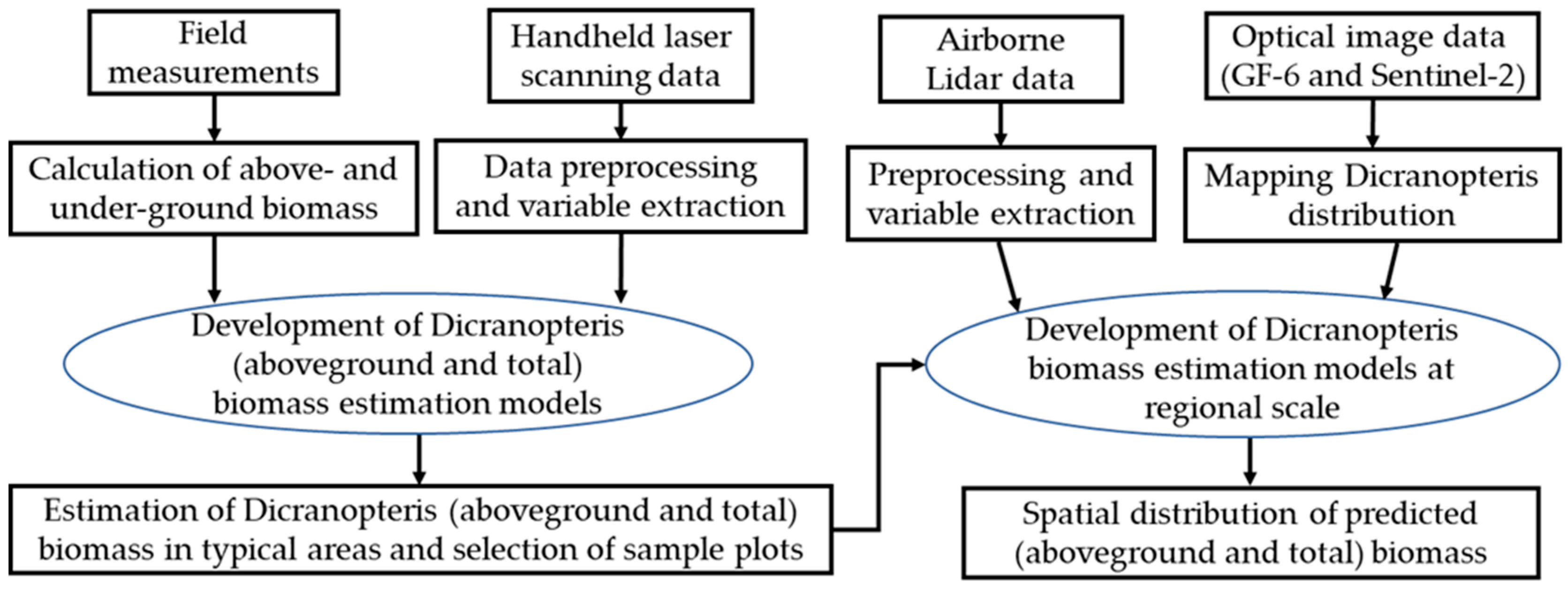
Figure 2 illustrates the framework for mapping Dicranopteris biomass distribution through a combination of field measurement, HLS, and ALS data. The major steps include (1) collection of aboveground and belowground biomass; (2) collection of HLS data at typical areas, covering the field survey plots, and the development of biomass estimation models based on the integration of field measurements and HLS data; (3) collection of ALS data covering the entire study area and development of biomass estimation models based on the integration of HLS-derived biomass data and ALS-derived variables; and (4) examination of spatial distribution of predicted aboveground and total biomass, and comparison of biomass difference between conservation and non-conservation regions.

3.1. Data Collection and Preprocessing

The datasets used in this research included field survey data, handheld and airborne laser scanning data, and other ancillary data, as summarized in Table 1. As indicated in this table, there was a few months difference between field measurements and Lidar data. However, considering the drought season and poor soil condition (due to long-term soil erosion) in this study area, the grass growth in this time period was very slow, thus, this short time difference between field measurement and Lidar data cannot significantly affect this research work.

3.1.1. Field Data Collection and Processing

The biomass harvesting method was used to collect Dicranopteris aboveground and belowground biomass during the field work [29]. According to Dicranopteris distribution and topographic conditions in this study area, 19 sample plots with a size of 1 m × 1 m were first allocated in August 2022 for collecting aboveground biomass. All Dicranopteris grasses above the ground within each sample plot were gleaned by cutting close to the ground and put into a labeled and sealed bag. To collect belowground biomass, Dicranopteris roots need to be dug out, which is a time-consuming and labor-intensive process for large plot sizes. Thus, a subplot with a size of 25 cm × 25 cm was set up at the center of each sample plot. All belowground Dicranopteris roots within each subplot were excavated by digging down to the rootless part of the Dicranopteris. The collected roots were cleaned with water to remove the dirt, and dried naturally, then put into a labeled and sealed bag. All sealed bags were brought into the lab, and put into a baking oven at 105 °C for 30 min, then lowered to 80 °C until reaching a constant weight. The dried grasses of each plot and the dried roots of each subplot were weighed and regarded as aboveground biomass (g/m2) and belowground biomass (g/0.0625 m2), respectively. Then, the biomass weight units were uniformly converted into t/ha. The total biomass of a sample plot was the sum of aboveground and belowground biomass. After initial examination of biomass distribution of 19 sample plots, 4 outliers were identified and removed from the sample dataset; thus, only 15 sample plots were used in model development (Section 3.2). Table 2 shows the statistics of biomass based on these samples.

3.1.2. Collection and Preprocessing of Airborne Laser Scanning (ALS) and Handheld Laser Scanning (HLS) Data

The ALS data covering the entire study area were collected in October 2022 using a Riegl VUX-240 Lidar system mounted on Trike AEROS-912 aircraft with flight height of 600 m, maximum scanning angle 75 degree, near-infrared band, and maximum scanning frequency of 1800 kHz. The ALS data had point density of over 50 pt/m2. The preprocessing of ALS data was conducted using LiDAR360 software, including mosaicking of point clouds, denoising, filtering, and normalizing [17]. The point cloud filtering was used to classify the Lidar point clouds into ground and non-ground points, the denoising tool was used to remove low points, air noise, and isolated points, and others like power lines that were identified visually and then removed. The ground points were used to produce digital elevation model (DEM) data with the inverse distance weighted interpolation method. The normalized point clouds were obtained through subtracting the DEM from object point elevation, thus removing the impacts of terrain features.
HLS data were collected using a LiGrip V100 laser sensor in November 2022. A total of 19 typical areas, each containing one sample plot, were collected within the ALS-covered area. The device used a laser with 903 nm spectral band, measured 300,000 pts/s, and had a scanning range of 100 m. To ensure all vegetation within the typical area were completely scanned, the field surveyor walked within the region with a zigzag way and multiple loops. The real-time kinematic (RTK) global positioning system receiver was used to collect control points for registering HLS data to the WGS 84-UTM zone 50 N coordinate system. The HLS data were preprocessed using LiFuser-BP software for inputting point cloud data, coordinate registration, denoising, filtering, and normalizing. Then, similar processing as used ALS was used for HLS data in Lidar360.

3.1.3. Mapping of Dicranopteris Distribution

Field survey on land-cover types were conducted in January and August 2022. A total of 212 samples with land-cover types including tree species and location information were collected. According to the landscape characteristics of this study area, the classification system includes Dicranopteris (Masson pine), agricultural lands, water body, impervious surface area, and others.
The GaoFen-6 (GF-6) panchromatic band with 2 m spatial resolution and Sentinel-2 data with 10 spectral bands, both of which were acquired on 15 February 2021, were used for land-use/cover classification. The GF-6 panchromatic band was orthorectified and then converted to surface reflectance using the dark-subtraction atmospheric calibration [30]. The Sentinel-2 L1C product was atmospherically calibrated using the Sen2Cor tool [31], producing a new dataset consisting of 10 spectral bands with 10 m spatial resolution. The Gram–Schmidt fusion method [32,33] was used to integrate the GF-6 panchromatic band and Sentinel-2 multispectral data to generate a new dataset of 10 spectral bands with 2 m spatial resolution.
Previous research has indicated that an object-based classification approach can provide better accuracy than pixel-based classifiers when high spatial resolution images are used [34]. Thus, this research used a multi-scale segmentation approach to convert spectral bands into segments [35]. Based on iterated experiments of segmentation, the scale parameter of 120, shape weight of 0.1, and compactness weight of 0.5 were finally selected. Based on the segment image, the fused images with 10 spectral bands and 2 m spatial resolution were used to extract the spectral images using the mean algorithm and the textural images using the gray-level co-occurrence matrix (GLCM, including entropy, homogeneity, contrast, second moment, mean, standard deviation, and dissimilarity) [36]. The modified hierarchy-based classifier [37] was then used to conduct the land-cover classification. The classification result was evaluated using confusion metrics [38]. Overall accuracy and kappa coefficient were used to evaluate the classification result, and user’s and producer’s accuracies were used to evaluate individual classes [39].
Because of the relatively simple stand structure and high separability of Masson pine with other land-cover types in this study area, the Masson pine was accurately classified with an accuracy of almost 100%. Considering that Dicranopteris was distributed under Masson pine forest, the classified result for Masson pine in this study was regarded as the same spatial distribution of Dicranopteris.

3.2. Dicranopteris Biomass Estimation with Handheld Laser Scanning (HLS) Data

Based on our field survey and the characteristics of Dicranopteris in height, we removed the Lidar points with height values greater than 1.2 m; thus, the remaining points belong to Dicranopteris. With the central point of the sample plot as the center, we created square windows with different sizes, from 1 m × 1 m to 8 m × 8 m, with an interval of 1 m, and extracted height percentile variables and density variables from the point clouds for each window size. Both height percentile variables and density variables depict the vertical structure of vegetation [40]. The height percentiles indicate the height values of Lidar points below which a certain percentage of the points are accounted for. To calculate height percentiles, all normalized Lidar point clouds within a given window size are sorted by the height from the lowest to the highest. Then, the height at i% (Hi) was calculated using a formula n = Hi × N, where N is the total number of Lidar points within the window, and n is the ordinal rank of a given value i. In this study, we calculated 19 height percentiles, from H10 to H95 at 5-intervals, and H99. To calculate the density variables, the point clouds were divided into 10 equal layers between the minimum and maximum heights within a given window size first, then, the density of the layer j (Dj) is the ratio of the number of points falling into the layer j (Aj) to the total number of points within the window (Aall), while j represents the layer number from 0 to 9, corresponding to the lowest to the highest layer [41].
Considering the number of extracted variables from point cloud data was larger than the number of samples, Pearson’s correlation coefficient was used to analyze the relationships between biomass and the extracted variables (i.e., percentile and density) for the removal of the variables with very weak relationships with biomass while having very high coefficients between the variables. After that, the stepwise regression method was used to develop estimation models for aboveground and total biomass. Except for linear regression models, we also created models similar to the allometric equations using Dj and Hi, which were identified in the best-fit regression models. The results were then evaluated using the leave-one-out cross-validation method. The coefficient of determination (R2), root mean square error (RMSE), and relative root mean square error (rRMSE) were calculated and used to evaluate the modeling results [42]. Through comprehensive evaluation among these modeling results based on different window sizes, the best model was finally selected for predicting aboveground and total biomass for the typical areas based on the HLS data.

3.3. Dicranopteris Biomass Estimation with Airborne Lidar Data

The research focus of this study was to estimate Dicranopteris biomass; thus, there was a need to remove any trees within the ALS data. The point clouds that had height values of greater than 1.2 m were deleted. Another concern was the selection of mapping size. Usually, the sample size of field measurements for trees is 20 m × 20 m. Therefore, the size with 20 m by 20 m was used to extract modeling variables from the ALS point clouds. Like the variables generated from the HLS data, the percentile and density variables were extracted from ALS data, too. The same methods used in HLS-based biomass modeling and result evaluation were used for ALS data for developing Dicranopteris biomass estimation models and evaluating the results.

4. Results

4.1. Analysis of Dicranopteris Biomass Estimation at Plot Level Using HLS Data

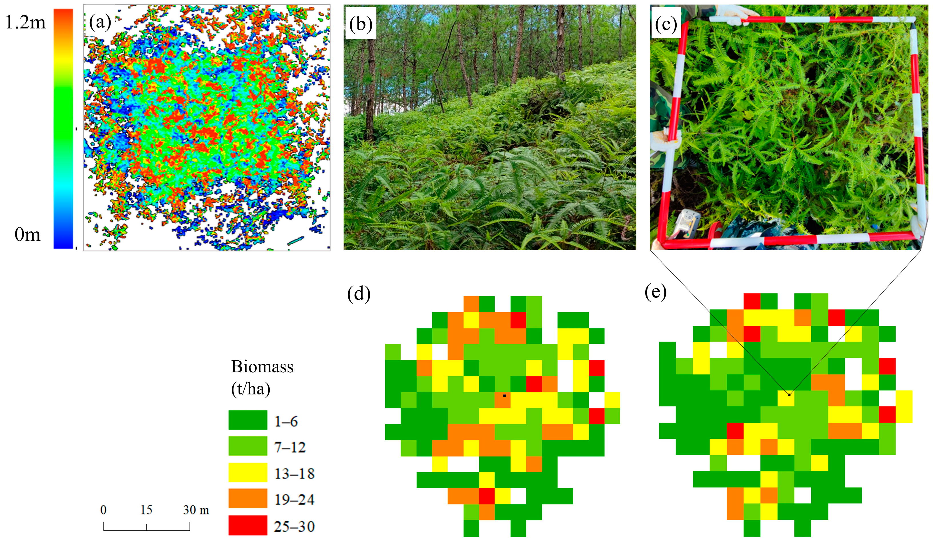
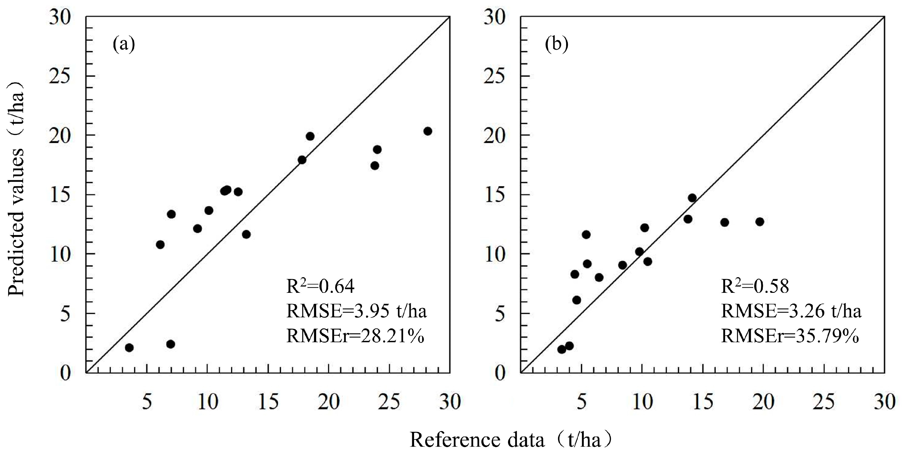
After a comparison of the estimation models and evaluation results, the best model for each window size was chosen, summarized in Table 3, indicating that modeling performance improved as window size increased until it reached its best size of 6 m by 6 m for both aboveground and total biomass modeling. One interesting thing in Table 3 implies that the combined use of both height percentile and density provides better modeling performance than the use of a single variable alone. In particular, the multiplicative combinations of density and height percentile had better performance than separate use of variables. The best models were applied to estimate total biomass and aboveground biomass for all HLS typical areas. As shown in Figure 3, the biomass distribution within the HLS region appears heterogeneous, and the high biomass variation indicates the important role of the HLS data in capturing the complex Dicranopteris spatial features. The scatter plots as shown in Figure 4 indicate good modeling performance, but the underestimation problem is obvious when biomass is relatively high, such as larger than 15 t/ha for aboveground biomass or 20 t/ha for total biomass.
Based on the predicted biomass using the selected models for the HLS data, a total of 19 samples were extracted from the HLS-estimated biomass, at the locations of the field sample plots, and used to connect ALS-derived variables. The statistics of selected samples are summarized in Table 4. Comparing with the statistical results of field measurements in Table 2, the results in Table 4 have a slightly larger range, but the mean and standard deviation are similar, indicating the good predicting results based on HLS data. These samples were used as modeling samples for developing total and aboveground biomass estimation models using ALS data from the entire study area.

4.2. Analysis of Dicranopteris Biomass Estimation with ALS Data

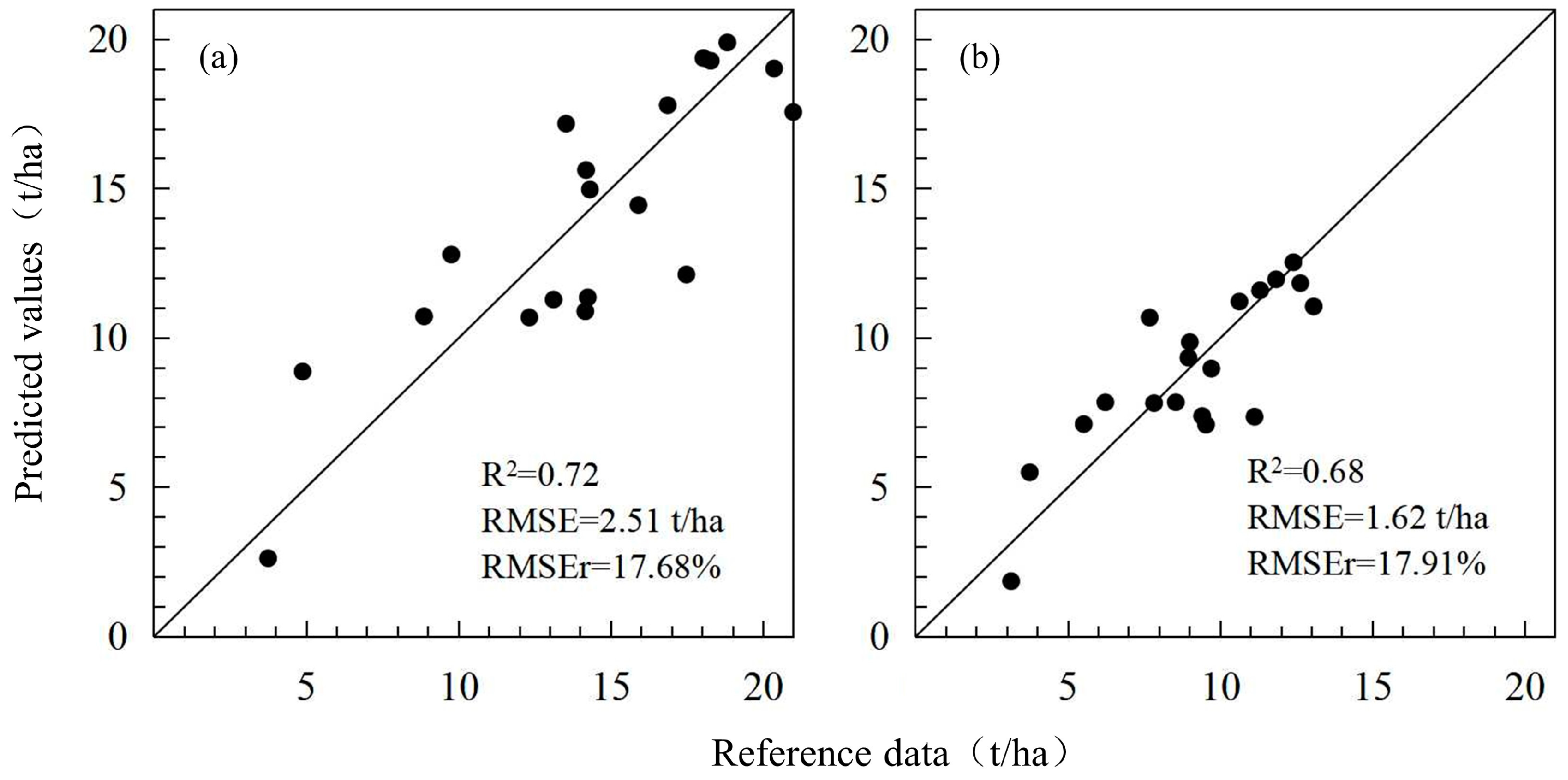
The modeling results based on ALS data show good prediction performance using both density and height percentile variables (Table 5). The rRMSE for both total and aboveground biomass prediction were less than 18%. The scatter plots (See Figure 5) show no obvious over- or under-estimation problems based on ALS data. A comparison of modeling results based on HLS (Table 3) and on ALS (Table 5) shows the importance of combining both height percentile and density in Dicranopteris biomass estimation modeling.
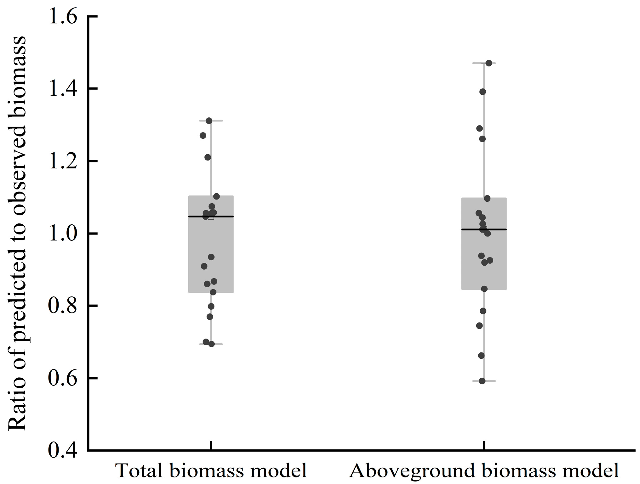
Figure 6 provides a visual comparison showing the distribution of the ratio of modelled biomass to observed biomass. For both models, the mean and median of ratios were basically around 1.0. However, for the total biomass model, ratio values were more centralized, while for the aboveground biomass model, the ratio values were much dispersed. This implied the total biomass model performed better than the aboveground biomass model.
The best models (Table 5) were used to predict total and aboveground biomass distribution for the entire study area (Figure 7), showing that total or aboveground biomass were mainly located in southwestern and eastern areas of the study area, while the northwestern and northern regions had relatively low biomass distribution. The total biomass amounts were mainly in 16–25 t/ha and aboveground biomass in 8–16 t/ha.

5. Discussion

5.1. Impacts of Plot Sizes on Biomass Modeling Performance

The design of a suitable plot size for field measurement needs to consider the representative and workload during the field survey. In general, a plot size of 20 m by 20 m or 1 mu (a unit of area of 0.0667 hectares) is often used in China’s forest inventory considering tree density and field survey conditions in mountainous regions. In this case, the surveyors mainly measure DBH for calculation of aboveground biomass using existing allometric equations [13]. However, for grass biomass calculation, the common variables are grass density (or coverage) and height if the specific allometric equation is available. Otherwise, a plot size of 1 m × 1 m is often used during field measurement for collection of aboveground or belowground biomass. In this study, we do not have allometric equations to directly calculate Dicranopteris biomass, thus, we used the harvesting method based on a small plot size such as 1 m by 1 m to collect aboveground biomass, and a nested subplot to collect belowground biomass. However, this small plot size may be not big enough to represent the Dicranopteris spatial patterns considering the complex spatial patterns of the understory vegetation, as showing in Figure 3 with the high heterogeneity of Dicranopteris coverage and height. This generates a problem on how to relate the variables based on a small plot size to remotely sensed data. The extracted variables based on different window sizes may have different values, thus, they may have various relationships with biomass. There is a need to identify a suitable size to relate the extracted variables to biomass so that the best relationship between the variables and biomass can be developed. In this research, we found that a window size of 6 m × 6 m was best for relating biomass to extracted variables for Dicranopteris when HLS data were used. However, caution should be taken when other data sources such as ALS or high-resolution optical sensor data are used. More research is needed to identify the best window size for a specific data source considering the complexity of understory vegetation and the spatial resolution of used remotely sensed data, or point density of the Lidar data.

5.2. The Important Role of HLS Data as a Bridge for Regional Biomass Estimation Modeling

Use of sample plots for biomass estimation modeling often faces two challenges: the sufficient number of samples and spatially good representativeness, which is often difficult for collection of sample plots in field work. In general, sample plots from field measurements are directly used as modeling samples for developing biomass estimation models based on remote sensing data, even Lidar data [13,17]. However, the limited number of sample plots for modeling often results in relatively poor performance, especially when the model is used for prediction in the study area due to the fact that sample plots lack representation. As UAVs are easily available for the collection of high-density point clouds, this makes it possible to produce many sample plots from the Lidar-derived biomass estimates. The Lidar-derived results provide new opportunities to develop robust models in a large area [43] through the collection of a sufficient number of samples that cannot be found in previous research. Previous research has shown the effectiveness of using ALS data for relating field sample plots to other remotely sensed data for forest biomass modeling in a large area [43]. However, ALS data cannot effectively capture understory vegetation features for directly modeling its biomass. This research explored the use of HLS data as a bridge to relate between field measurement and ALS data for estimation of Dicranopteris biomass, which creates new ways to estimate the understory biomass. More research is needed to further improve the modeling performance by incorporating ancillary data such as DEM and soil conditions, considering the fact that soil erosion in this study area seriously affects the restoration of understory vegetation.

6. Conclusions

This research selected the Luodihe watershed in Changting County as a case study to examine the method to estimate the understory, total, and aboveground Dicranopteris biomass in a subtropical region, using the integration of field measurements, and HLS and ALS data. This research found that a small plot size of 1 m by 1 m may be suitable for collection of aboveground and belowground biomass during field survey, but this small size has relatively poor representation in spatial scale, resulting in poor modeling performance. A window size of 6 m by 6 m is suitable for relating HLS data with sample plots for developing the total and aboveground biomass model using a linear regression approach based on the extracted height percentile and density variables. The HLS data play an important role in relating sample plots and ALS data for accurately developing regional biomass estimation models. This research provides a new way to map the spatial distribution of Dicranopteris biomass through a combination of limited field measurement, and HLS and ALS data. The results from this research will be valuable for evaluating the effects of implementing conservation measures on improving the degraded ecosystem functions and services and provides important data sources for local government to make proper decisions for managing and protecting the ecosystem.

Author Contributions

Conceptualization, D.L. (Dengsheng Lu), J.W. and S.L.; methodology, D.L. (Dengsheng Lu), D.L. (Dengqiu Li), X.L., J.W. and S.L.; software, X.L.; validation, D.L. (Dengqiu Li) and X.L.; formal analysis, X.L.; investigation, D.L. (Dengqiu Li), S.L. and X.L.; resources, D.L. (Dengsheng Lu), D.L. (Dengqiu Li), J.W. and S.L.; data curation, D.L. (Dengqiu Li) and X.L.; writing—original draft preparation, X.L. and D.L. (Dengsheng Lu); writing—review and editing, D.L. (Dengsheng Lu), J.W., S.L. and D.L. (Dengqiu Li); visualization, D.L. (Dengsheng Lu) and D.L. (Dengqiu Li); supervision, D.L. (Dengsheng Lu); project administration, D.L. (Dengsheng Lu) and D.L. (Dengqiu Li); funding acquisition, D.L. (Dengsheng Lu), J.W., S.L. and D.L. (Dengqiu Li). All authors have read and agreed to the published version of the manuscript.

Funding

This research was funded by Fujian Provincial Science and Technology Department, grant number 2021R1002008, the Department of Water Resources of Fujian Province, grant numbers MSK202207 and MSK202311, and the Ministry of Water Resources, grant number SKS-2022083.

Data Availability Statement

Data sources such as field surveys can be obtained from Dengsheng Lu at Fujian Normal University upon request.

Acknowledgments

The authors would like to thank Ruoqi Wang, Yunhe Li, and Shitao Li for their support during the collection of field measurements and handheld scanning data.

Conflicts of Interest

The authors declare no conflicts of interest. The funders had no role in the design of the study; in the collection, analyses, or interpretation of data; in the writing of the manuscript; or in the decision to publish the results.

References

  1. Deng, H.; Lin, Q.; Teng, H.; Zhao, Y.; Deng, Y. Analysis on the Growth Regularity of Dicranopteris Dichotoma in Areas of Intensive Soil Erosion. J. Fujian For. Coll. 2004, 24, 262–264. [Google Scholar]
  2. Liu, Y.; Liu, Q.; Wang, H.; Ma, Z.; Xu, W. Distribution Characteristics of Dicranopteris Dichotoma Biomass. J. Ecol. 2008, 5, 705–711. [Google Scholar]
  3. Chen, N.; Zhang, Q.; Chen, T.; Yang, Y.; Xie, J. Stoichiometric Characteristics of Nitrogen and Phosphorus in Dicranopreris dichotoma During Ecosystem Restoration of Eroded Red-Soil. For. Res. 2016, 29, 735. [Google Scholar]
  4. Hou, X.; Han, H.; Tigabu, M.; Cai, L.; Meng, F.; Liu, A.; Ma, X. Changes in Soil Physico-Chemical Properties Following Vegetation Restoration Mediate Bacterial Community Composition and Diversity in Changting, China. Ecol. Eng. 2019, 138, 171–179. [Google Scholar] [CrossRef]
  5. Li, Q.; Zhu, C.; Yu, J.; Wu, X.; Huang, S.; Yang, F.; Tigabu, M.; Hou, X. Response of Soil Bacteria of Dicranopteris Dichotoma Populations to Vegetation Restoration in Red Soil Region of China. J. Soil Sci. Plant Nutr. 2023, 23, 456–468. [Google Scholar] [CrossRef]
  6. Chen, Y.; Liu, Z.; Rao, X.; Wang, X.; Liang, C.; Lin, Y.; Zhou, L.; Cai, X.; Fu, S. Carbon Storage and Allocation Pattern in Plant Biomass among Different Forest Plantation Stands in Guangdong, China. Forests 2015, 6, 794–808. [Google Scholar] [CrossRef]
  7. Wan, S.; Zhang, C.; Chen, Y.; Zhao, J.; Wang, X.; Wu, J.; Zhou, L.; Lin, Y.; Liu, Z.; Fu, S. The Understory Fern Dicranopteris Dichotoma Facilitates the Overstory Eucalyptus Trees in Subtropical Plantations. Ecosphere 2014, 5, art51. [Google Scholar] [CrossRef]
  8. Chen, W.; Su, F.; Pang, Z.; Mao, Q.; Zhong, B.; Xiong, Y.; Mo, J.; Lu, X. The Removal of Understory Vegetation Can Rapidly Alter the Soil Microbial Community Structure without Altering the Community Assembly in a Primary Tropical Forest. Geoderma 2023, 429, 116180. [Google Scholar] [CrossRef]
  9. Ren, Y.; Lü, M.; Jiang, J.; Xie, J. Effects of Dicranopteris Dichotoma on Soil Dissolved Organic Carbon in Severely Eroded Red Soil. Acta Ecol. Sin. 2018, 38, 2288–2298. [Google Scholar]
  10. Deng, C.; Chen, Z.; Chen, H.; Chen, Z. Hyperspectral Estimation Model of Chlorophyll Content of Dicranopteris Dichotoma under Different Ecological Restoration Years in Changting County in the Red Soil Erosion Area of Southern China. ISPRS Int. J. Geo-Inf. 2019, 21, 948–957. [Google Scholar]
  11. Yang, L.; Huang, Y.; Lima, L.V.; Sun, Z.; Liu, M.; Wang, J.; Liu, N.; Ren, H. Rethinking The Ecosystem Functions of Dicranopteris, A Widespread Genus of Ferns. Front. Plant Sci. 2021, 11, 581513. [Google Scholar] [CrossRef] [PubMed]
  12. Wang, J.; Zhang, M.; Yi, L.; Zhang, R.; He, Y. Effects of Light and Nitrogen on Clonal Reproduction Characteristics and Biomass Allocation of Dicranopteris dichotoma. J. Zhejiang A F Univ. 2021, 38, 74–83. [Google Scholar]
  13. Lu, D.; Chen, Q.; Wang, G.; Liu, L.; Li, G.; Moran, E. A Survey of Remote Sensing-Based Aboveground Biomass Estimation Methods In Forest Ecosystems. Int. J. Digit. Earth 2016, 9, 63–105. [Google Scholar] [CrossRef]
  14. Ma, T.; Zhang, C.; Ji, L.; Zuo, Z.; Beckline, M.; Hu, Y.; Li, X.; Xiao, X. Development of Forest Aboveground Biomass Estimation, Its Problems and Future Solutions: A Review. Ecol. Indic. 2024, 159, 111653. [Google Scholar] [CrossRef]
  15. Sinha, S.; Jeganathan, C.; Sharma, L.K.; Nathawat, M.S. A Review of Radar Remote Sensing for Biomass Estimation. Int. J. Environ. Sci. Technol. 2015, 12, 1779–1792. [Google Scholar] [CrossRef]
  16. Alappat, V.O.; Joshi, A.K.; Krishnamurthy, Y.V.N. Tropical Dry Deciduous Forest Stand Variable Estimation Using SAR data. J. Indian. Soc. Remote Sens. 2011, 39, 583–589. [Google Scholar] [CrossRef]
  17. Lu, D.; Jiang, X. A brief overview and perspective of using airborne lidar data for forest biomass estimation. Int. J. Image Data Fus. 2024, 15, 1–24. [Google Scholar] [CrossRef]
  18. Akay, A.E.; Oğuz, H.; Karas, I.R.; Aruga, K. Using LiDAR Technology in Forestry Activities. Environ. Monit. Assess. 2009, 151, 117–125. [Google Scholar] [CrossRef] [PubMed]
  19. Guan, H.; Su, Y.; Sun, X.; Xu, G.; Li, W.; Ma, Q.; Wu, X.; Wu, J.; Liu, L.; Guo, Q. A Marker-Free Method for Registering Multi-Scan Terrestrial Laser Scanning Data in Forest Environments. ISPRS J. Photogramm. Remote Sens. 2020, 166, 82–94. [Google Scholar] [CrossRef]
  20. Reich, K.F.; Kunz, M.; Von Oheimb, G. A New Index of Forest Structural Heterogeneity Using Tree Architectural Attributes Measured by Terrestrial Laser Scanning. Ecol. Indic. 2021, 133, 108412. [Google Scholar] [CrossRef]
  21. Panagiotidis, D.; Abdollahnejad, A.; Slavík, M. 3D Point Cloud Fusion from UAV and TLS to Assess Temperate Managed Forest Structures. Int. J. Appl. Earth Obs. 2022, 112, 102917. [Google Scholar] [CrossRef]
  22. Guo, Q.; Su, Y.; Hu, T. Lidar Principles, Processing and Applications in Forest Ecology; Higher Education Press: Beijing, China, 2018; (In Chinese). ISBN 9787040493016. [Google Scholar]
  23. Mokany, K.; Raison, R.J.; Prokushkin, A.S. Critical Analysis of Root: Shoot Ratios in Terrestrial Biomes. Glob. Chang. Biol. 2006, 12, 84–96. [Google Scholar] [CrossRef]
  24. IPCC. 2019 Refinement to the 2006 IPCC Guidlines for National Greenhouse Gas Inventories; IPCC National Greenhouse Gas Inventories Programme: Hayama, Japan, 2019; Volume 4. [Google Scholar]
  25. Reich, P.B.; Luo, Y.; Bradford, J.B.; Poorter, H.; Perry, C.H.; Oleksyn, J. Temperature Drives Global Patterns in Forest Biomass Distribution in Leaves, Stems, and Roots. Proc. Natl. Acad. Sci. USA 2014, 111, 13721–13726. [Google Scholar] [CrossRef] [PubMed]
  26. Wang, P.; Heijmans, M.M.P.D.; Mommer, L.; Van Ruijven, J.; Maximov, T.C.; Berendse, F. Belowground Plant Biomass Allocation in Tundra Ecosystems and Its Relationship with Temperature. Environ. Res. Lett. 2016, 11, 055003. [Google Scholar] [CrossRef]
  27. Ma, H.; Mo, L.; Crowther, T.W.; Maynard, D.S.; Van Den Hoogen, J.; Stocker, B.D.; Terrer, C.; Zohner, C.M. The Global Distribution and Environmental Drivers of Aboveground versus Belowground Plant Biomass. Nat. Ecol. Evol. 2021, 5, 1110–1122. [Google Scholar] [CrossRef]
  28. Li, Z.; Li, Q.; Hou, X.; Huang, Z.; Liu, Q.; Chen, S.; Zhao, Y. Characteristics of Soil and Water Loss in Pinus Massoniana Forest with Different Canopy Density under Different Natural Rainfall Levels. J. Soil. Water Conserv 2020, 34, 27–33+40. [Google Scholar]
  29. Kato-Noguchi, H. Involvement of Allelopathy in the Formation of Monospecific Colonies of Ferns. Nat. Prod. Commun. 2015, 10, 1934578X1501000. [Google Scholar] [CrossRef]
  30. Lu, D.; Batistella, M.; Moran, E. Multitemporal Spectral Mixture Analysis for Amazonian Land-Cover Change Detection. Can. J. Remote Sens. 2004, 30, 87–100. [Google Scholar] [CrossRef]
  31. Louis, J.; Debaecker, V.; Pflug, B.; Main-Knorn, M.; Bieniarz, J.; Mueller-Wilm, U.; Cadau, E.; Gascon, F. Sentinel-2 SEN2COR: L2A Processor for Users. In Proceedings of the Living Planet Symposium, Prague, Czech Republic, 9–13 May 2016. [Google Scholar]
  32. Karathanassi, V.; Kolokousis, P.; Ioannidou, S. A Comparison Study on Fusion Methods Using Evaluation Indicators. Int. J. Remote Sens. 2007, 28, 2309–2341. [Google Scholar] [CrossRef]
  33. Brodu, N. Super-Resolving Multiresolution Images with Band-Independent Geometry of Multispectral Pixels. IEEE Trans. Geosci. Remote Sens. 2017, 55, 4610–4617. [Google Scholar] [CrossRef]
  34. Lu, D.; Hetrick, S.; Moran, E. Land Cover Classification in a Complex Urban-Rural Landscape with QuickBird Imagery. Photogramm. Eng. Remote Sens. 2010, 76, 1159–1168. [Google Scholar] [CrossRef] [PubMed]
  35. Xie, Z.; Chen, Y.; Lu, D.; Li, G.; Chen, E. Classification of Land Cover, Forest, and Tree Species Classes with ZiYuan-3 Multispectral and Stereo Data. Remote Sens. 2019, 11, 164. [Google Scholar] [CrossRef]
  36. Yu, X.; Lu, D.; Jiang, X.; Li, G.; Chen, Y.; Li, D.; Chen, E. Examining the Roles of Spectral, Spatial, and Topographic Features in Improving Land-Cover and Forest Classifications in a Subtropical Region. Remote Sens. 2020, 12, 2907. [Google Scholar] [CrossRef]
  37. Jiang, X.; Zhao, S.; Chen, Y.; Lu, D. Exploring Tree Species Classification in Subtropical Regions with a Modified Hierarchy-Based Classifier Using High Spatial Resolution Multisensor Data. J. Remote Sens. 2022, 2022, 9847835. [Google Scholar] [CrossRef]
  38. Congalton, R.G.; Green, K. Assessing the Accuracy of Remotely Sensed Data: Principles and Practices, 2nd ed.; CRC Press: Boca Raton, FL, USA, 2008; ISBN 978-0-429-14397-7. [Google Scholar]
  39. Lu, D.; Weng, Q. A Survey of Image Classification Methods and Techniques for Improving Classification Performance. Int. J. Remote Sens. 2007, 28, 823–870. [Google Scholar] [CrossRef]
  40. Georgopoulos, N.; Gitas, I.Z.; Korhonen, L.; Antoniadis, K.; Stefanidou, A. Estimating Crown Biomass in a Multilayered Fir Forest Using Airborne LiDAR Data. Remote Sens. 2023, 15, 2919. [Google Scholar] [CrossRef]
  41. Wang, R.; Li, G.; Lu, Y.; Lu, D. A Comparative analysis of Grid-Based and Object-Based Modeling Approaches for Poplar Forest Growing Stock Volume Estimation in Plain Regions Using Airborne Lidar Data. Geo-Spat. Inf. Sci 2023, 1–19. [Google Scholar] [CrossRef]
  42. Cao, L.; Xu, T.; Shen, X.; She, G. Mapping Biomass by Integrating Landsat OLI and Airborne Lidar Transect Data in Subtropical Forests. J. Remote Sens. 2016, 20, 665–678. [Google Scholar]
  43. Jiang, X.; Li, G.; Lu, D.; Chen, E.; Wei, X. Stratification-Based Forest Aboveground Biomass Estimation in a Subtropical Region Using Airborne Lidar data. Remote Sens. 2020, 12, 1101. [Google Scholar] [CrossRef]
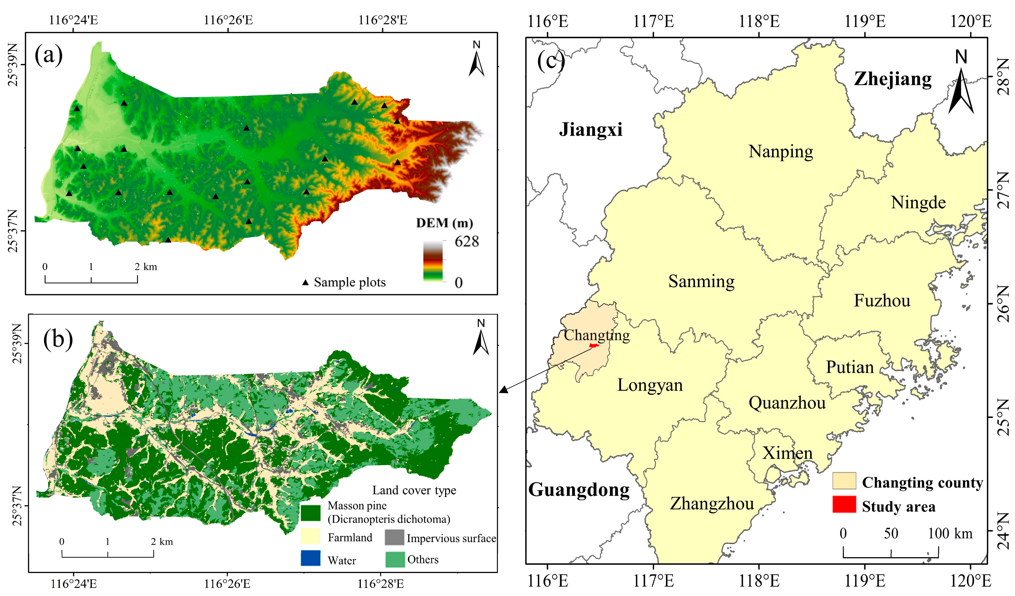
Figure 1. Study area (a): Elevation distribution of the Luodihe watershed with overlaid sample plots; (b): distribution of major land cover types, including Dicranopteris dichotoma under Masson pine forest; (c): the highlighted study area in red color, in Changting County, Fujian Province, China.
Remotesensing 16 02088 g001
Figure 2. Framework of mapping Dicranopteris biomass distribution through integration of field measurements, handheld laser scanning, and airborne laser scanning data.
Remotesensing 16 02088 g002
Figure 3. The spatial distributions of predicted biomass within the HLS region (a): point clouds within the HLS area showing the height heterogeneity of Dicranopteris distribution; (b): the picture showing Dicranopteris distribution under Masson pine for the HLS area; (c): an example to show the collection of aboveground biomass within the plot size of 1 m × 1 m; (d): the predicted total biomass distribution at a window size of 6 m × 6 m; (e): the predicted aboveground biomass distribution at a window size of 6 m × 6 m.
Remotesensing 16 02088 g003
Figure 4. The scatter plots between the modeling results from HLS and field measurements based on total biomass (a) and aboveground biomass (b), showing the underestimation problem when biomass was relatively high.
Remotesensing 16 02088 g004
Figure 5. The relationship between the predicted biomass values and corresponding reference data (a): total biomass; (b): aboveground biomass.
Remotesensing 16 02088 g005
Figure 6. Distribution of the ratio of predicted biomass using developed models to observed biomass for total and aboveground biomass.
Remotesensing 16 02088 g006
Figure 7. Spatial distribution of the Dicranopteris dichotoma biomass (a): total biomass distribution, (b): aboveground biomass.
Remotesensing 16 02088 g007
Table 1. Datasets used in research.
DatasetsDescription
Field survey of land-cover typesLand-cover types, including Masson pine forest with understory vegetation of Dicranopteris, farmland, water, impervious surfaces, and others were collected in January and August 2022.
Field measurement at plot level19 sample plots with a size of 1 m × 1 m for collection of Dicranopteris aboveground biomass, and 19 subplots with a size of 25 cm × 25 cm at the center of each 1 m × 1 m plot for collection of root biomass were collected in August 2022. The unit of belowground, aboveground, and total biomass with g/m2 for each sample was then converted to t/ha.
Handheld laser scanning data19 typical areas containing the sample plots were collected in November 2022 using the handheld laser scanning device.
Airborne laser scanning dataAirborne Lidar data covering the entire Luodihe Watershed were collected in October 2022.
Optical sensor dataRemote sensing images including GaoFen-6 (GF-6) panchromatic band with 2 m spatial resolution and Sentinel-2 multispectral bands with 10 m spatial resolution were collected; both images were acquired in February 2021.
Table 2. Biomass statistics of sample plots (t/ha).
Category Range (t/ha)Mean (t/ha) Standard Deviation (t/ha)
Aboveground biomass4.0–19. 709.204.97
Belowground biomass 1.50–14.034.823.67
Total biomass6.11–28.1614.036.87
Table 3. Comparison of modeling results using HLS data based on different window sizes.
Biomass (g/m2)Window Size
(m2)
Estimation ModelsModeling
R2m
Evaluation
Validation
R2v
RMSE
(t/ha)
rRMSE
(%)
Total biomass1 × 128.48 − 3.97H75 − 73.88 D20.270.076.7147.85
3 × 3−7.31 + 12.07 H99 + 98.60 D50.140.068.0957.70
4 × 423.26 − 22.65 H95 + 178.02 D50.500.216.1443.84
5 × 512.73 − 26.27 H80 + 275.81 D50.760.614.3030.63
6 × 60.88 + 1410 D52H99 0.850.643.9528.21
7 × 70.46 + 1450 D52H99 0.780.584.2029.97
8 × 8−6.13 − 26.54 H10 + 318.92 D50.720.474.6433.14
Above-ground biomass1 × 113.69 + 3.87 H80 − 40.71 D20.340.194.3647.39
3 × 30.47 + 7.98 H50 + 54.83 D50.210.056.0665.86
4 × 4−2.25 + 8.63 H10 + 115.02 D50.430.154.3246.89
5 × 51.41 − 8.50 H80 + 174.49 D50.570.323.9642.98
6 × 62.15 + 3250 D52H10 0.840.583.2635.79
7 × 72.39 + 3090 D52H10 0.800.344.9053.28
8 × 81.45 + 3730 D52H10 0.790.214.7851.92
Note: Dj represents density of the jth layer and Hn represents the nth height percentile, R2m and R2v represent coefficient of determination based on model and evaluation, respectively.
Table 4. Statistics of sample data extracted from modeling results using the handheld laser scanning data based on the plot size of 20 m × 20 m.
Biomass CategoryRange (t/ha)Mean (t/ha)Standard Deviation (t/ha)
Aboveground biomass1.15–24.208.685.62
Total biomass1.89–25.4214.146.82
Table 5. Modelling results based on ALS data and sampling plot data.
Estimation ModelsModeling
R2m
Evaluation Results
Validation
R2v
RMSE
(t/ha)
rRMSE
(%)
Total biomass −1.38 + 11.43H75 + 131.12D40.8240.722.5117.68
Aboveground biomass−0.95 + 5.49H90 + 82.58D40.7840.681.6217.91
Note: Dj represents density of the jth layer and Hn represents the nth height percentile, R2m and R2v represent coefficient of determination based on model and evaluation, respectively.
Disclaimer/Publisher’s Note: The statements, opinions and data contained in all publications are solely those of the individual author(s) and contributor(s) and not of MDPI and/or the editor(s). MDPI and/or the editor(s) disclaim responsibility for any injury to people or property resulting from any ideas, methods, instructions or products referred to in the content.