Reconstruction of Hourly FY-4A AGRI Land Surface Temperature under Cloud-Covered Conditions Using a Hybrid Method Combining Spatial and Temporal Information

Abstract

Land Surface Temperature (LST) products obtained by thermal infrared (TIR) remote sensing contain considerable blank areas due to the frequent occurrence of cloud coverage. The studies on the all-time reconstruction of the cloud-covered LST of geostationary meteorological satellite LST products are relatively few. To accurately fill the blank area, a hybrid method for reconstructing hourly FY-4A AGRI LST under cloud-covered conditions was proposed using a random forest (RF) regression algorithm and Savitzky-Golay (S-G) filtering. The ERA5-Land surface cumulative net radiation flux (SNR) reanalysis data was first introduced to represent the change in surface energy arising from cloud coverage. The RF regression method was used to estimate the LST correlation model based on clear-sky LST and the corresponding predictor variables, including the normalized difference vegetation index (NDVI), the normalized difference water index (NDWI), surface elevation and slope. The fitted model was then applied to reconstruct the cloud-covered LST. The S–G filtering method was used to smooth the outliers of reconstructed LST in the temporal dimension. The accuracy evaluation was performed using the measured LST of the representative meteorological stations after scale correction. The coefficients of determination derived with the reference LST were all above 0.73 on the three examined days, with a bias of −1.13–0.39 K, mean absolute errors (MAE) of 1.46–2.4 K, and root mean square errors (RMSE) of 1.77–3.2 K. These results indicate that the proposed method has strong potential for accurately restoring the spatial and temporal continuity of LST and can provide a solution for the production and research of gap-free LST products with high temporal resolution.

1. Introduction

Land Surface Temperature (LST) is one of the most important parameters for regional and global energy exchange, and the radiative balance of the surface–atmosphere system. The temporal and spatial information of Land Surface Temperature has not only been widely used to study the urban heat island effect, detect geothermal resources, and monitor fire points, but it also directly affects important parameters like soil moisture and surface evapotranspiration [1,2,3,4,5]. Satellite-based thermal infrared (TIR) remote sensing plays an important role in quickly obtaining large-scale LST, due to its direct relationship with the thermal remote sensing signal [6,7,8]. Many thermal infrared sensors can provide high-precision LST datasets. However, due to the inability of thermal radiation to penetrate clouds, many LST products contain considerable blank areas due to the frequent occurrence of cloud coverage, which seriously destroys the spatial and temporal continuity of LST and limits the application of LST products. Given the importance of LST, it is essential to accurately estimate the LST of cloud-covered pixels and restore the spatial and temporal continuity of LST products.

Currently, three main methods have been developed to fill the missing values of LST resulting from cloud coverage [9]. Spatial information-based methods are based on the high correlation between the cloud-covered LST and the adjacent clear-sky LST, or the predictor variables of LST. Neteler (2010) used Kriging interpolation to interpolate and fill the gap in MODIS LST datasets considering the gradient relationship of clear-sky LST [10]. Ke et al. (2013) used the Regression Kriging (RK) to interpolate and reconstruct the cloud-covered LST in large-scale mountainous areas [11]. Simple statistical approaches can interpolate the missing values of LST datasets. Nevertheless, these approaches fail to consider the physical relationships of environmental variables between surface and atmosphere. Therefore, interpolated results tend to be hypothetical clear-sky LST instead of actual cloudy-sky LST [12]. Considering the disadvantages of the simple statistical methods, Jin and Dickinson (2000) proposed a physical algorithm to reconstruct cloud-covered skin temperature based on the surface energy balance (SEB) equation [13]. The equation was constructed through land surface energy terms, including sensible heat flux, latent heat flux, canopy and soil energy, surface net solar radiation and surface net longwave radiation. Each term of the SEB was first expressed as a function of skin temperature, then the SEB was solved to derive cloud-covered skin temperature from neighboring clear-sky skin temperature. This algorithm is suitable for LST reconstruction at night and high latitudes. However, the values of the energy terms in SEB are difficult to obtain, and the accuracy of the algorithm depends on the accuracy of the clear-sky skin temperature and the input parameters. With the rapid development of artificial intelligence, machine learning has recently shown a tremendous ability to capture the spatial relationship of variables and reconstruct missing data in remote sensing [14,15]. Considering the advantages of the random forest (RF) in finding the nonlinear relationship between LST and its predictor variables, Zhao and Duan (2020) proposed a method to estimate the actual daytime cloud-covered MODIS LST by using RF regression algorithm [16]. The method estimated a cumulative downward surface solar radiation flux (DSSF) to represent the impact from cloud cover on incident solar radiation. Results indicated that RF has strong potential for reconstructing LST under cloud-covered conditions. Nevertheless, this method is only suitable for reconstructing a daytime LST image of a polar-orbiting satellite due to the lack of solar radiation in the nighttime. Moreover, when the spatial resolution is lower, the spatial correlation between LST and prediction variables is weakened, which makes it harder to accurately estimate cloud-covered LST with relatively low spatial resolution but high temporal resolution, such as geostationary meteorological satellite LST products. Therefore, further research is required in reconstructing the actual cloud-covered LST products of a geostationary meteorological satellite.

Multi-temporal information-based methods are based on the LST variation of target pixels in a time series to reconstruct cloud-covered LST. At the daily scale, the diurnal temperature cycle (DTC) model was first proposed by Parton and Logan (1981) and was further studied by Jin and Dickinson (1999) and Jin (2000) [17,18,19]. This model applied a daily scale interpolation to obtain diurnal LST cycles, thus recovering the cloudy-sky LST. At the annual scale, the annual temperature cycle (ATC) was proposed and applied to fill the missing values of Landsat long-term LST products [20]. The multi-temporal information-based methods have made extraordinary progress [21]. Nevertheless, the accuracy of the methods is closely related to factors such as surface conditions, model fitting ability, and optimal parameter selection, which may introduce additional errors in LST reconstruction and accuracy verification.

Hybrid methods were developed to fill the missing values, combining the spatial and temporal information of LST. Wang et al. (2021) proposed an algorithm that considered the spatial and temporal characteristics [22]. Firstly, using the similar characteristics of the adjacent time LST, the partial reconstruction of the FY-4A LST product was performed in the temporal dimension. Secondly, the normalized difference vegetation index (NDVI) was used to find similar pixels to the target pixels, and interpolation was performed to fill the gap. Finally, the preliminary reconstructed LST was denoised using a Savitzky–Golay (S–G) filter, thus realizing the reconstruction of the cloud-covered pixels of geostationary meteorological satellite LST products. However, this method did not consider the physical relationship between the surface and the atmosphere either; thus, the reconstruction results were hypothetical clear-sky LST. Wu et al. (2019) proposed a multiscale feature connection model using a convolutional neural network (CNN) [9]. This model achieves a high-accuracy reconstruction of high missing rate regions. However, the reconstruction method requires a lot of computing resources, and difficulties in batch data processing make this model less practical. Ding et al. (2022) proposed an RTG method integrating China Land Surface Data Assimilation System (CLDAS) reanalysis data and FY-4A TIR data for reconstructing hourly all-weather LST based on RF regression, the DTC model and the ATC model [23]. The method was applied to the Tibetan Plateau and the validation results indicated that the accuracy of the reconstructed all-weather LST was better than the CLDAS LST and FY-4A LST under clear-sky, cloudy-sky, and all-weather conditions.

In general, great progress has been achieved in this field. Nevertheless, there are some limitations of the proposed reconstruction methods that deserve to be noted, which can be listed as follows: (1) Due to the relatively low spatial resolution of geostationary meteorological satellite LST products and the negative effects of mixed pixels and the scale effect, it is quite difficult to verify the accuracy of the results by simply using ground measured LST. Therefore, studies on the reconstruction of geostationary meteorological satellite LST products under cloud-covered conditions are relatively few. (2) Because of the lack of consideration regarding the physical relationships of the environmental variables between the surface and atmosphere, the reconstruction results of cloud-covered LST in some methods were hypothetical clear-sky LST instead of actual cloudy-sky LST. (3) Due to the radiation balance and energy transfer mechanism of the surface being different at night than in the daytime, some methods are only applicable in the daytime rather than nighttime. In response to these challenges, this study aims to develop an all-time reconstruction method by combining the spatial and temporal information of LST and the surface energy balance theory, ensuring the recovery of the actual cloudy-sky LST of a geostationary meteorological satellite is attainable with reliable accuracy.

Based on the above considerations, the study proposed a hybrid method for reconstructing the Fengyun-4A (FY-4A) AGRI LST under cloud-covered conditions by combining the spatial and temporal information of LST. The ERA5-Land surface cumulative net radiation flux (SNR) reanalysis data was first introduced to represent the change in surface energy arising from cloud coverage. The RF regression method was used to estimate the LST correlation model based on clear-sky LST and the corresponding predictor variables, including the normalized difference vegetation index (NDVI), the normalized difference water index (NDWI), surface elevation and slope. The fitted model was then applied to reconstruct cloud-covered LST. The S–G filtering method was used to smooth the outliers of reconstructed LST in the temporal dimension. The proposed method was applied to Heilongjiang Province, Northeast China and the results of the validation were presented to verify its accuracy.

2. Materials and Methods

2.1. Study Area

Heilongjiang Province, China, shown in Figure 1, was selected as the study area. Heilongjiang Province is located in Northeast China (43°26′–53°33′N,121°11′–135°05′E). The terrain of this region is complex, including plains, mountains, etc. The altitude difference of the whole area can reach over 1600 m. As is shown in Figure 1, the land cover types of this region include cropland, forest, shrubbery, grassland, impervious, etc. The 30 m land cover data can be obtained from the website of China National Cryosphere Desert Data Center (http://www.ncdc.ac.cn/, accessed on 13 September 2023) [24]. Heilongjiang Province has an obvious temperate continental monsoon climate. In summer, it is warm and rainy due to the influence of the southeast monsoon. In winter, it is cold and dry due to the influence of the northwest monsoon. The diversity of terrain, land cover types and climate types in this region make the LST change greatly, and the spatial and temporal distribution has strong uncertainty. Therefore, the variability of the land thermal characteristics and their complex influencing factors make this region an ideal area for studying LST reconstruction methods.

2.2. Data

2.2.1. FY-4A AGRI L2 LST

The Fengyun-4A (FY-4A) satellite is a new generation of geostationary meteorological satellite launched in China on 11 December 2016. The sensor of an Advanced Geostationary Radiation Imager (AGRI) can perform full-disk detection every 15 min. AGRI has a total of 14 bands, including four long-wave infrared bands, and band 12 (10.3–11.3 μm) and band 13 (11.5–12.5 μm) are mainly to retrieve LST products by using the split-window algorithm. The LST products provided by the FY-4A AGRI have the characteristics of high temporal resolution and high accuracy. The AGRI LST has a spatial resolution of 4 km in NetCDF format, which can be downloaded for free from the Feng Yun Satellite Remote Sensing Data Network (https://satellite.nsmc.org.cn/, accessed on 10 April 2023). The study selects three days from different seasons (5 April 2021, 15 July 2021, 22 October 2021) as the research period, and downloads the hourly FY-4A AGRI L2 LST of these days from the website.

According to statistics, the average vacancy rate of LST on 5 April 2021 is 47.81%, of which the average vacancy rate during the day is 58.71%, and 34.74% at night; on 15 July 2021, the average vacancy rate of LST in the whole day was 79.60%, of which the average vacancy rate in the daytime was 87.13%, and 72.06% at night. The average vacancy rate of LST for the whole day on 22 October 2021 is 23.92%, of which the average vacancy rate during the day is 24.21%, and 23.63% at night.

2.2.2. Predictor Variables of LST

Land Surface Temperature is the product of land surface–atmosphere energy balance, which contains abundant geological information and represents the energy change in the interaction between land surface and atmosphere. The diurnal variation and spatial distribution of LST are affected by many factors, including atmospheric condition, surface albedo, land cover types, topographic condition, etc. [25]. These factors affect the balance of surface absorbing and emitting energy, thus affecting the value of LST. In the surface–atmosphere system, the direct driving force of the LST diurnal variation comes from the surface cumulative net radiation flux. The surface cumulative net radiation flux refers to the cumulative net radiation energy absorbed and emitted by the surface, which is an important part of the surface energy balance. In the temporal dimension, the surface mainly absorbs solar shortwave radiation during the day, making surface net radiation flux increase to a positive value. Therefore, daytime LST tends to show an upward trend. At night, the surface is dominated by upward long-wave radiation and the surface net radiation flux decreases to a negative value, which makes nighttime LST show a downward trend. In the spatial dimension, the main energy source of LST in the daytime is solar radiation. The presence of clouds blocking the solar radiation affects the change in the surface net radiation flux, resulting in the clear-sky LST being generally higher than cloudy-sky LST. Moreover, the surface is dominated by upward long-wave radiation at night. As for cloudy-sky pixels, clouds prevent the surface long-wave radiation from dissipating into space and retain the heat of the surface to a certain extent. In contrast, the long-wave radiation from the clear-sky pixels will be directly lost to space, resulting in a quicker decrease in LST. Therefore, the cloudy-sky LST at night will generally be higher than the clear-sky LST. In conclusion, the surface cumulative net radiation flux takes into account the shielding effect of clouds and the reflection and thermal radiation of clouds, and can accurately represent the change in actual cloudy-sky LST. The study first introduced the surface cumulative net radiation into the LST reconstruction model, as the lead impact factor in recovering the actual cloud-covered LST.

In addition to the surface cumulative net radiation flux, different land cover types also have different effects on LST. In general, areas with more vegetation cover usually have a lower LST, because vegetation can absorb solar radiation and release heat through transpiration. Conversely, bare land or urban areas usually have a higher LST because they can absorb more solar radiation and store heat. Moreover, water bodies can also affect LST. Water bodies have a high heat capacity, which can absorb and release a large amount of heat, thereby reducing the LST of the surrounding area. Therefore, the study selects the normalized difference vegetation index (NDVI) and the normalized difference water index (NDWI) to quantitatively describe the impact of different land cover types on LST.

Moreover, LST has a close relationship with the terrain. The LST in high altitude areas is relatively low, because higher altitudes can lead to changes in atmospheric pressure and humidity, thus resulting in low atmospheric temperature and weak solar radiation, which in turn affect LST. Additionally, the surface slope also affects LST. Surface slope greatly controls the amount of direct solar radiation received by the land surface through the angle between the normal surface slope and the solar beam [26]. To quantify the terrain effect on LST, the study selects surface elevation (ELV) and surface slope (SLP) as the predictor variables. The selected remote sensing datasets are shown in

Table 1. Introduction of the remote sensing data in this study.

Data	Spatial Resolution	Usage
FY-4A AGRI L2 LST	4 km	As the target of this study
ERA5-Land reanalysis data (SNSR, SNLR, DSSR)	0.1°	As the radiation factor of LST
MOD09A1 8-day synthetic reflectance data	500 m	As the spectral factor of LST
MOD13A2 16-day synthetic NDVI data	1 km
ASTER GDEM V3 surface elevation data	30 m	As the topographic factor of LST
Measured LST of meteorological stations	/	As the reference LST for accuracy validation
Land cover data	30 m	As the reference data to select representative meteorological stations

.

• ERA5-Land Reanalysis Data

Compared with polar-orbiting satellite products, reanalysis data has the advantage of spatio-temporal continuity [27]. The reanalysis of global land surface (ERA5-Land) products, carried out by the fifth-generation European center for medium-range weather forecasts (ECMWF), is simulated by the modified land surface model HTESSEL [28]. Compared with previous generations, ERA5-Land reanalysis datasets have higher accuracy and resolution. ERA5-Land provides global hourly surface data from 1950 to the present, which can be downloaded for free on the European Copernicus Meteorological Data website (https://cds.climate.coprnicus.eu/, accessed on 15 April 2023). In this study, the hourly data of ERA5-Land surface cumulative net short-wave radiation (SNSR), surface cumulative net long-wave radiation (SNLR), and downward cumulative surface solar radiance (DSSR), covering the study area at the corresponding time of AGRI LST, were selected as the radiation influencing factors of LST, the spatial resolution of which is 0.1° × 0.1°. Moreover, in this study, the surface cumulative net short-wave radiation and the surface cumulative net long-wave radiation value are added together as the surface cumulative net radiation (SNR), which acts as the actual radiation influence factor of LST.

• MODIS Data

The Moderate-Resolution Imaging Spectroradiometer (MODIS) is a sensor mounted on both Aqua and Terra satellites. It has 36 visible and infrared wavebands with a wide spectral range of 0.4–14.4 μm. In this study, MOD09A1 500 m 8-day synthetic reflectance data was used to calculate the NDWI of the study area, and MOD13A2 1 km 16-day synthetic NDVI data was used as the surface spectral influence factor of the study area. The MODIS data can be downloaded from the NASA LAADS DAAC website for free (https://ladsweb.modaps.osdis.nasa.gov/, accessed on 15 April 2023).

• ASTER GDEM Data

Terrain has a great influence on the spatial distribution and variation of LST. The height, slope, aspect, and topography of the terrain all affect the reception and reflection of solar radiation, resulting in large differences in LST on different terrains. Therefore, it is necessary to obtain high-precision terrain data to describe the influence of terrain on LST. This study selected the ASTER global digital elevation model (GDEM) Version 3 dataset, which can be downloaded from the NASA Earthdata website (https://urs.earthdata.nasa.gov/, accessed on 15 April 2023) for free, with a spatial resolution of 30 m. The DEM data are used to calculate the slope, and the surface elevation and slope are used as the terrain influence factors of LST.

2.2.3. LST Measurements of Meteorological Stations

To evaluate the accuracy of the proposed LST reconstruction model, this study obtained hourly measured LST observation data from 82 meteorological stations in Heilongjiang Province to verify the accuracy of cloud-covered pixel reconstruction LST. The LST data are measured on the flat and loose bare land surface in the observation field of the meteorological stations, and have undergone strict quality control, which has good representativeness and reliability.

2.3. Methods

2.3.1. Flowchart Description

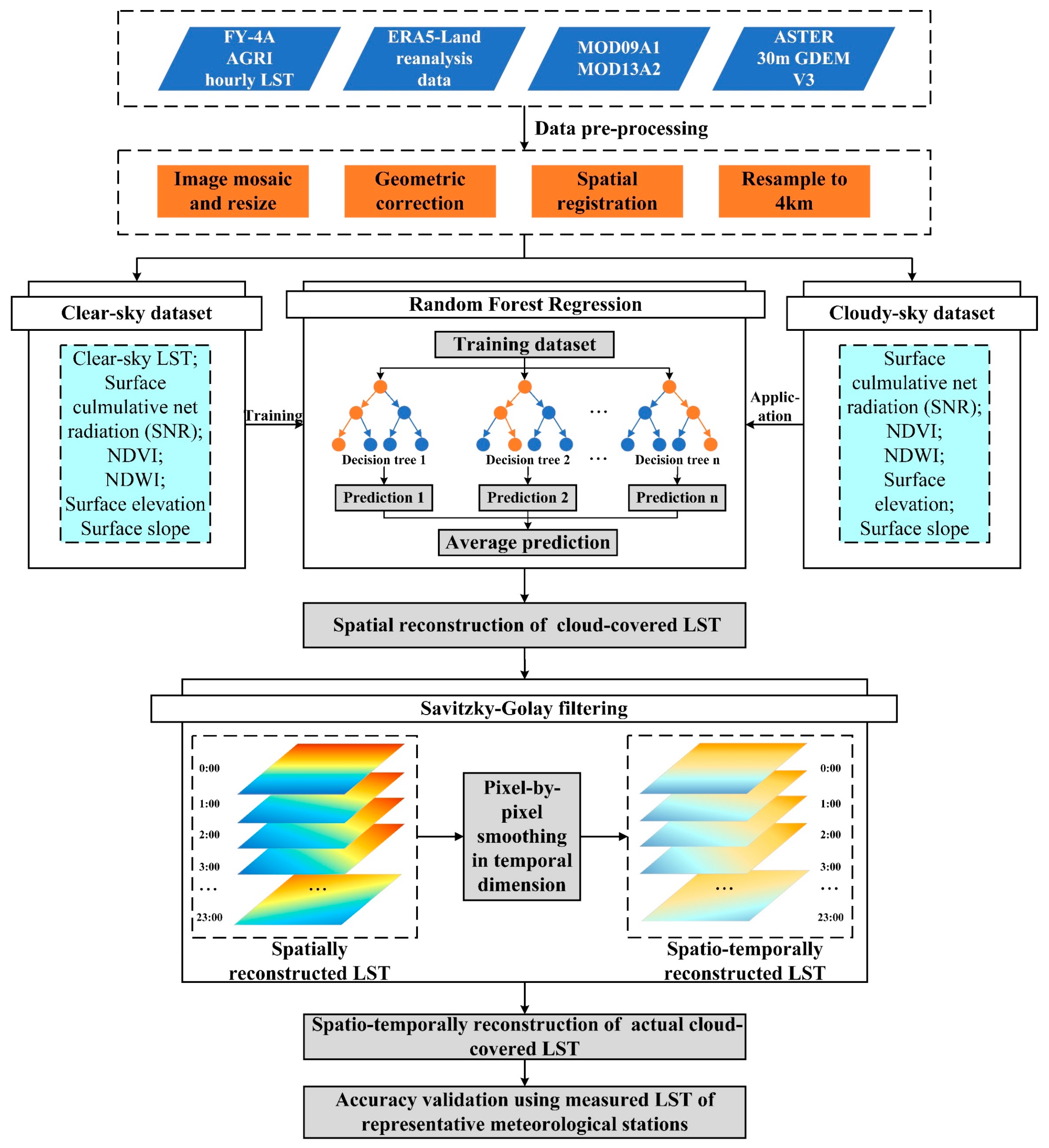
The flowchart of the hybrid reconstruction method for FY-4A AGRI LST under cloud-covered conditions is shown in Figure 2. The main steps include: (1) Data preprocessing: including geometric correction of AGRI LST, spatial registration of LST predictor variables, and resampling to 4 km spatial resolution using bilinear interpolation. (2) LST correlation model: The clear-sky LST is used as the target variable, and the corresponding predictor variables (SNR, NDVI, NDWI, ELV, SLP) are used as the predictors of LST to train the random forest correlation model. Then the trained random forest correlation model is applied to cloudy-sky pixels to recover LST. (3) Temporal smoothing: For each pixel, the Savitzky–Golay filtering is used to smooth the temporal dimension to remove the LST outliers. (4) Accuracy assessment: This involves using the representative meteorological station measured LST after spatial scale correction as the reference LST to evaluate the accuracy of LST reconstruction results, so as to explore the reliability of the LST reconstruction model proposed in this study.

2.3.2. LST Correlation Model Based on Random Forest Regression

Land Surface Temperature is the result of surface energy balance, which is affected by atmospheric environment, land cover types, terrain conditions and other factors. The cumulative net surface radiation flux is a direct manifestation of the surface energy budget, including the absorption and reflection of short-wave radiation, and the absorption and emission of long-wave radiation, which plays a decisive role in the change in LST. The coverage of clouds significantly changes the surface energy balance, blocking the surface to receive short-wave radiation from the sun and long-wave radiation emitted from the surface. Meanwhile, it also emits upward and downward thermal radiation, which greatly changes the surface energy balance and then affects the change in LST. Among the input factors used to fit the model, except for the surface cumulative net radiation flux, the remaining predictors remain almost unchanged in one day. The reconstruction result based on these unchanged predictive variables is the hypothetical clear-sky LST. The surface cumulative net surface radiation flux considers the shadowing effect and the reflection and radiation transmission of clouds, so it can accurately represent the change in LST under both clear-sky and cloudy-sky conditions in the whole time period. To quantitatively describe the nonlinear relationship between LST and its predictor variables, the LST correlation model can be established as follows [29]:

$$\{\begin{array}{c}LS{T}_{actual}=LS{T}_{est}+e\\ LS{T}_{est}=f\left(V_{SNR},V_{NDVI},V_{NDWI},V_{ELV},V_{SLP}\right)\end{array}$$

(1)

where ${\mathrm{LST}}_{\mathrm{actual}}$ is the actual cloud-covered LST; ${\mathrm{LST}}_{\mathrm{est}}$ is the estimated cloud-covered LST; e is the error of the correlation model; f is a function that correlates the nonlinear relationship between LST and its impact variables. The predictor variables include surface cumulative net radiation ${\mathrm{V}}_{\mathrm{SNR}}$, the normalized difference vegetation index ${\mathrm{V}}_{\mathrm{NDVI}}$, the normalized difference water index ${\mathrm{V}}_{\mathrm{NDWI}}$, surface elevation ${\mathrm{V}}_{\mathrm{ELV}}$ and surface slope ${\mathrm{V}}_{\mathrm{SLP}}$. The surface cumulative net radiation is obtained by adding the surface cumulative net short-wave radiation flux to the surface cumulative net long-wave radiation flux.

The core idea of LST reconstruction is to explore the relationship between LST and its predictor variables. Due to the complex relationship between LST and its predictor variables, it is difficult to construct a suitable numerical model to reflect this relationship. Therefore, this study uses the Random Forest regression model in machine learning to fit the nonlinear relationship between LST and its predictor variables, thus constructing the LST correlation model. The random forest regression algorithm is an ensemble learning model based on the decision tree algorithm [30]. Multiple decision trees are constructed by randomly selecting a subset of training samples to form a random forest, and the average value is used to improve the prediction accuracy and prevent the model from overfitting [31]. When fitting the LST correlation model using the RF regression model, the impact of the surface net radiation flux and other variables on clear-sky LST can be learned via the correlation model. Due to the existence of an intersection between clear-sky LST and cloudy-sky LST with respect to the influencing mechanism of cloud coverage on LST [16], the influencing mechanism of the predictor variables on clear-sky LST should also be applicable to cloud-covered pixels. Therefore, when the LST correlation model is extended to cloud-covered conditions, the impact of predictor variables can be effectively quantified and the actual cloudy-sky LST can be predicted.

Before fitting the random forest regression model, the optimal hyperparameter setting of the random forest regression algorithm is as follows: the number of decision trees is 500, the maximum depth of decision trees is 20. The clear-sky LST and the corresponding predictor variable value of 70% are used as the training set, and the value of 30% is used for the test set. The cross-validation method is used to select the optimal model, and then the trained model is applied to the cloud-covered pixels. The predictor variables of the cloud-covered pixels are used to calculate the actual LST under cloud-covered conditions.

2.3.3. Temporally Smoothing Based on S–G Filtering Method

In addition to the characteristics of spatial distribution, the variation characteristics of LST in the temporal dimension are also obvious. LST reconstruction based on the random forest regression algorithm is a spatial information-based LST reconstruction method. Although it can fill the missing value of FY-4A AGRI LST products, this method only considers the spatial distribution characteristics of LST but does not consider the temporal variation characteristics, which makes it difficult to ensure the continuity and variation characteristics of the reconstructed LST in the temporal dimension. Therefore, it is necessary to smooth the LST reconstruction results in the temporal dimension, to process the discrete values of the spatial dimension reconstruction, reduce the error of the correlation model, and further improve the reconstruction accuracy and reliability.

Savitzky–Golay (S–G) filtering is a filtering method based on local polynomial least squares fitting in the temporal dimension, which was first proposed by Savitzky and Golay in 1964 [32]. By selecting a fixed number of objects in the adjacent time phase of the filtering object for polynomial fitting, and using the least squares to select the optimal polynomial of the fitting effect, its value at the filtering object is the S–G filtering smoothing result. The S–G filtering process can be expressed as follows:

$$LS{T}_i^{\prime }=\frac{{{\displaystyle \sum }}_{j=-m}^m{k}_{j}LS{T}_{i+j}}{N}$$

(2)

where ${\mathrm{LST}}_{\mathrm{i}}^{\prime }$ is the smoothed LST result; ${\mathrm{LST}}_{\mathrm{i}+\mathrm{j}}$ is the original value of LST; m is the width of filtering window; N is the amount of data in the filtering window, whose value is equal to (2 m + 1); and k_j is the corresponding weight of the jth LST original value in the filtering window.

In this study, the LST value of each pixel is extracted by time phase. The polynomial order is determined to be 2, the window width m is determined to be 9 after plenty of tests.

2.3.4. Selection of Representative Meteorological Stations and Scale Conversion of Measured LST

To verify the accuracy of the reconstructed LST, hourly LST observation data from 82 meteorological stations across Heilongjiang Province were selected as the reference LST. However, the low spatial resolution of geostationary meteorological satellite LST leads to a more serious mixed pixel effect. Consequently, the scale discrepancy between the reconstructed LST and the reference LST makes it less reliable to compare them directly. To evaluate the accuracy of the AGRI LST reconstruction results more reliably using measured LST data, it is necessary to select meteorological stations with better spatial representation and convert their measured LST to the correct spatial scale, so as to eliminate the scale discrepancy between meteorological stations and remote sensing observations as much as possible.

• Selection of Representative Meteorological Stations

Representative meteorological stations should be characterized by a relatively homogeneous underlying surface surrounding the station, with minimal variation in land cover types. This homogeneity ensures that the measurements are reflective of consistent and representative samples of the local atmospheric conditions, thereby enhancing the accuracy and reliability of the ground measured LST. Therefore, to elevate the reliability of the reference LST, it is critical to conduct the selection of representative meteorological stations.

To better quantify the representativeness of the meteorological stations, the study employed the 30 m land cover data of Heilongjiang Province obtained from the China National Cryosphere Desert Data Center [24]. With the pixel housing the meteorological stations as the center, a rectangular search window was established with a side length of 4 km. Within this window, the number of land cover types that differ from that of the center pixel, where the meteorological stations were located, was tallied. A lower count of different land cover types within the search window indicates a higher degree of homogeneity, suggesting that the LST measured at this meteorological station is more reliable and representative.

2.

Scale Conversion of Measured LST

Due to the relatively small spatial scale of the measured LST data at the representative meteorological stations, in order to make the reference LST and reconstructed LST more comparable, it is necessary to perform scale conversion on the measured LST. The measured LST at the representative meteorological stations and the LST observed by satellites tend to show a similar variation trend in both the spatial and temporal dimensions. Therefore, there is a relatively obvious linear relationship between them. Taking the clear-sky LST of a FY-4A pixel corresponding to the location of the representative meteorological station as the reference LST, the linear correction model of the measured LST can be established as follows:

$$LS{T}_{FY-4A}=a\times LS{T}_{station}+b$$

(3)

where a and b are linear regression coefficients; ${\mathrm{LST}}_{\mathrm{station}}$ is the measured LST of the representative meteorological stations, and ${\mathrm{LST}}_{\mathrm{FY}-4\mathrm{A}}$ is the LST corresponding to the FY-4A pixel where the station is located. Considering the different spatial and temporal distribution and variation of LST during the day and night, this study established the scale conversion model during the day and night, respectively.

2.4. Accuracy Variation Method

After the selection of representative meteorological stations and the scale conversion of measured LST, the corrected measured LST is used as the reference temperature to evaluate the accuracy of the reconstructed LST results of cloud-covered pixels. The quantitative evaluation indicators include the coefficient of determination R-square (${\mathrm{R}}^2$), bias, mean absolute error (MAE) and root mean square error (RMSE).

3. Results

3.1. Results of Selecting Representative Meteorological Stations and Scale Conversion of Measured LST

Based on the spatial representative analysis of 82 meteorological stations in Heilongjiang Province, 50 stations are selected to evaluate the accuracy of reconstruction results. After selection, the linear regression model is used to scale the hourly measured LST on 15 April, 15 July, and 22 October 2021. The measured LST before and after the scale correction are compared with the LST corresponding to the FY-4A clear-sky pixels where the stations are located, and the coefficient of determination ${\mathrm{R}}^2$ and the root mean square error (RMSE) are calculated to evaluate the scale conversion effect. The scale conversion results are shown in

Table 2. The result of the scale correction of the three-day hourly measured LST by representative meteorological stations using simple linear model. The gains (a) and offsets (b) represent linear regression coefficients in Equation (3).

Date		Samples	Gains (a)	Offsets (b)	R2	RMSE (K) before Correction	RMSE (K) after Correction
5 April 2021	Daytime	313	0.69	82.17	0.74	7.59	3.19
	Nighttime	356	0.61	103.90	0.63	3.27	1.51
15 July 2021	Daytime	133	0.13	254.70	0.35	21.22	1.64
	Nighttime	173	0.41	169.60	0.30	7.72	1.93
22 October 2021	Daytime	409	0.71	77.89	0.85	5.03	2.19
	Nighttime	452	0.46	145.50	0.22	2.97	1.90

. It can be seen from Table 2 that the average coefficients of determination of the three-day scale conversion results total 0.52, and the average RMSE after scale conversion is about 2 K, which is significantly lower than the RMSE before conversion (8 K in average), indicating that the effect of the linear scale conversion model is satisfactory. Because of the high missing rate of LST, the coefficients of determination of the scale transformation are relatively lower throughout the whole day of 15 July and the night of 22 October.

3.2. Reconstruction of Hourly FY-4A AGRI Cloudy-Sky LST

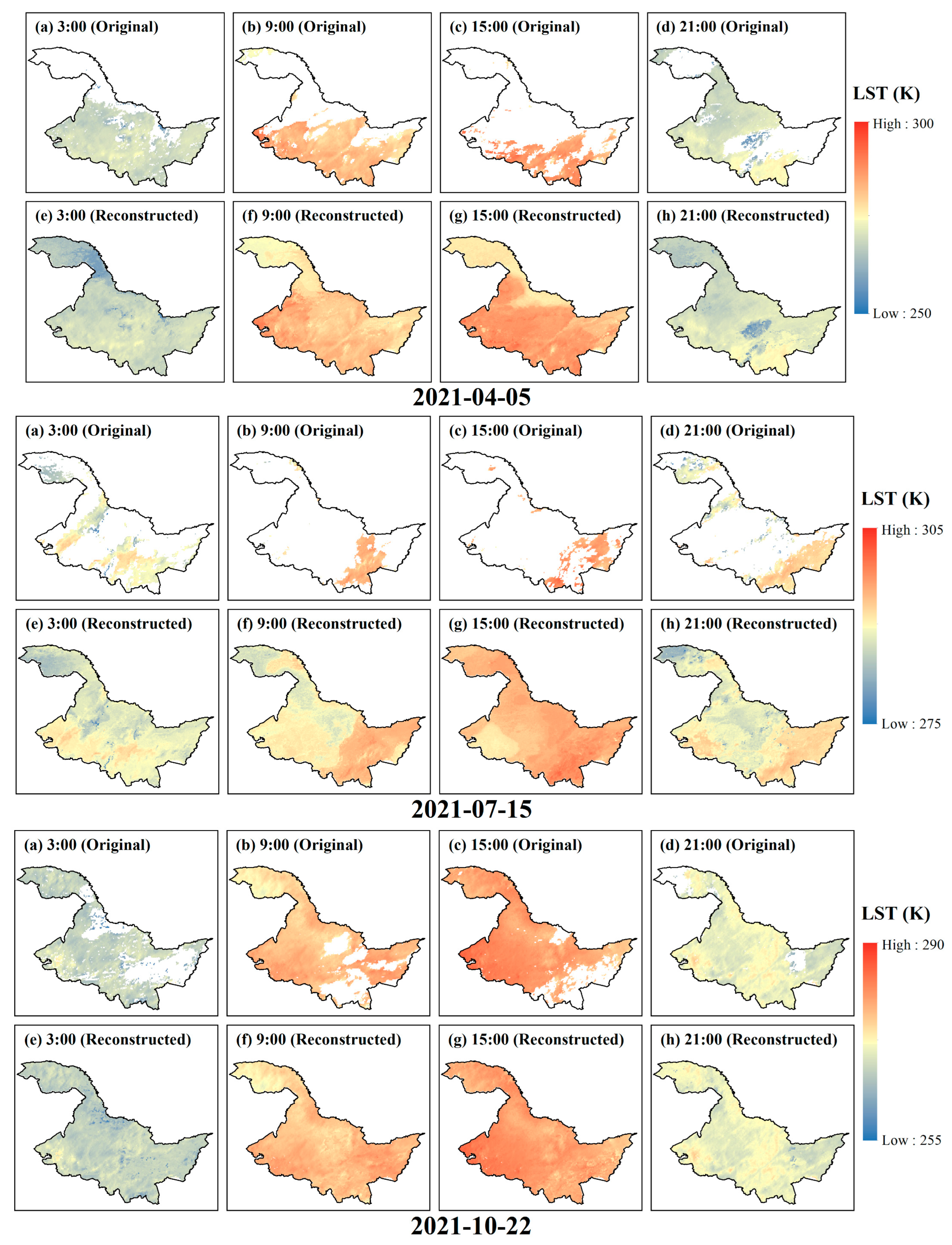
In this study, the proposed method is used to reconstruct the hourly FY-4A AGRI LST under cloud-covered conditions on 5 April, 15 July, and 22 October 2021, and S–G filtering is used to process the discrete values at the temporal dimension. Taking the four moments of 3:00, 9:00, 15:00 and 21:00 (UTC+8) as examples, the results are shown in Figure 3.

Figure 3 shows the gap-filled LST of FY-4A AGRI on 5 April, 15 July, and 22 October. It can be obviously seen that the proposed hybrid LST reconstruction model based on the random forest regression algorithm and S–G filtering shows a satisfactory result. Through visual interpretation, it is obvious that the LST reconstruction results are continuous in the spatial dimension, and the outliers can be corrected by S–G filtering without obvious abrupt points and boundaries. In the temporal dimension, LST generally shows a downward-upward-downward trend, and the temporal changes in LST in different seasons have different characteristics. The temperature difference in LST in the morning and evening in spring and autumn is larger, while the temperature difference in LST in the morning and evening in summer is smaller.

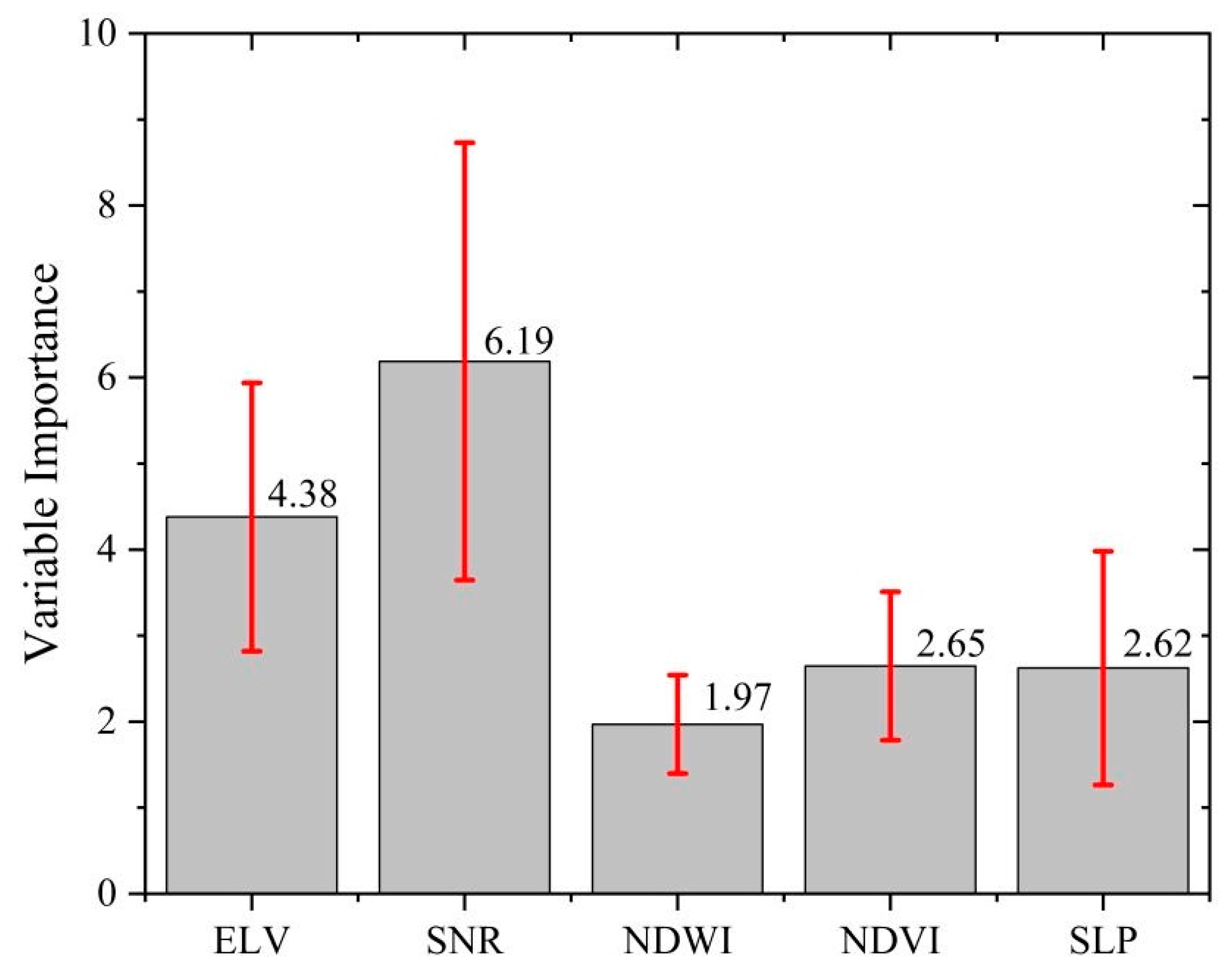
The random forest regression algorithm can not only construct the LST correlation model to predict the LST of cloud-covered pixels, but also provide the variable score to show the contribution of the selected predictor to LST. The higher the score, the more important the predictor is. Figure 4 shows the average score and standard deviation of the variable importance of each selected predictor variables on the selected three days. Among all the predictors, the score of the surface cumulative net radiation flux (SNR) is the highest (the average score of which is 6.19), because the surface cumulative net radiation flux directly determines the surface energy budget and has a controlling effect on the change in LST. The score of surface elevation (ELV) comes second, the average score of which is 4.38. The terrain of Heilongjiang Province is complex, and the changes between different terrains are obvious. Therefore, the surface elevation also has a significant controlling effect on LST. In contrast, the importance of surface slope (SLP) is relatively low (the average score is 2.62). This is because Heilongjiang Province is dominated by plain terrain, and the terrain is not undulating, so the control effect of surface slope on LST is not particularly obvious. Among the prediction variables, the scores of the surface spectral variables (NDVI and NDWI) are relatively low, indicating that for Heilongjiang Province, the control effect of the surface spectral factors on LST is not particularly obvious. Among the spectral factors, the average score of NDWI is the lowest, which is 1.97 points. This is because the water distribution in Heilongjiang Province is generally less, and most of the water bodies are covered by clouds at the imaging time. Therefore, the correlation model trained by clear-sky pixels cannot represent the influence of water bodies on LST well.

3.3. Methods Comparison

During the daytime, since the surface receives shortwave radiation from the sun as an energy source for the increase in LST, Zhao and Duan (2020) used the cumulative downward surface solar radiation flux (DSSR) to characterize the effect of cloud duration on LST changes, and then used the random forest regression algorithm to reconstruct cloudy-sky LST in the spatial dimension [16]. In this study, the surface–atmosphere energy balance process is considered, and the surface cumulative net radiation flux (SNR) is used to replace DSSR to realize the reconstruction of LST under cloud-covered conditions throughout the day. Therefore, it is necessary to evaluate the LST reconstruction effect of the two methods during the daytime.

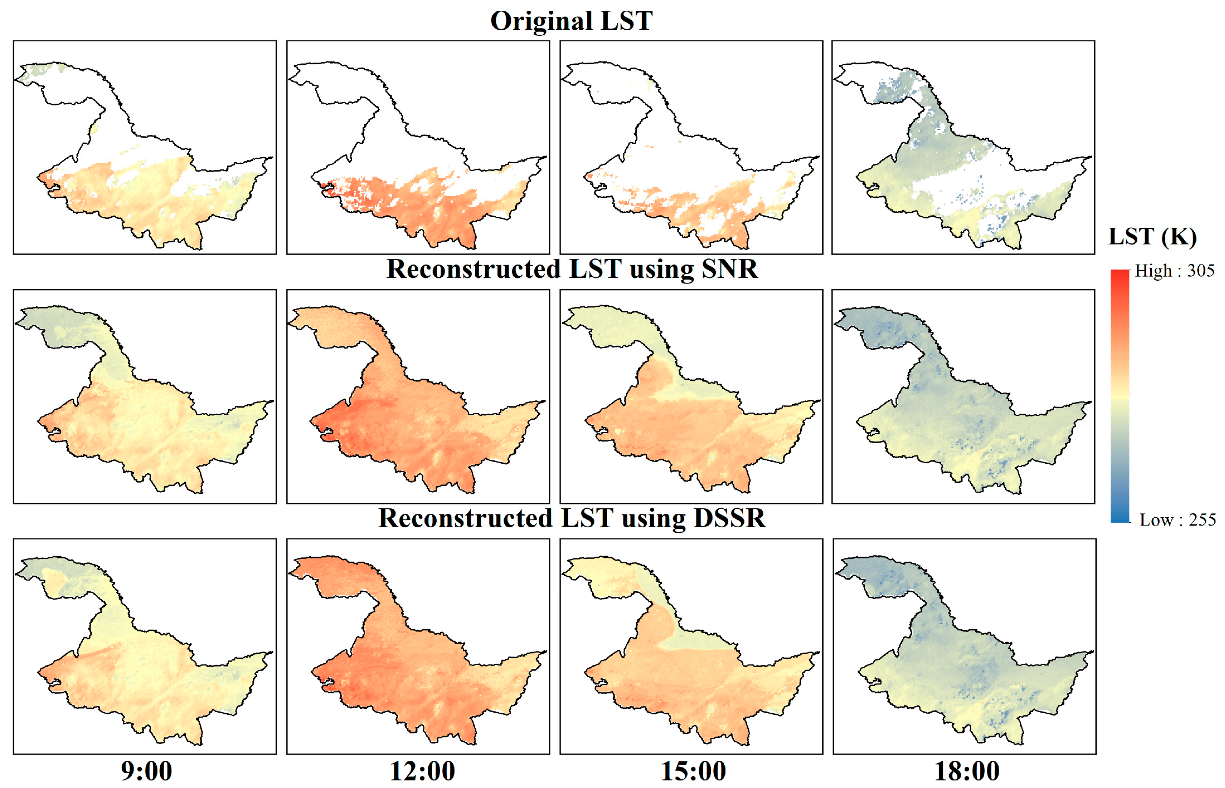
Taking the FY-4A AGRI LST from 9:00 to 18:00 (UTC+8) on 5 April with a relatively low missing rate as an example, SNR and DSSR are selected as radiation predictor variables in the LST correlation model, and other impact parameters remain the same. The results of LST reconstruction by these two radiation factors are compared. The results are shown in Figure 5, and the accuracy evaluation results, compared with the measured LST data of meteorological stations after linear correction, are shown in Figure 6.

From the reconstruction results of Figure 5, it can be obviously seen that both the cumulative net radiation flux (SNR) and the cumulative downward solar radiation flux (DSSR) can be used to reconstruct the missing values of FY-4A AGRI LST under cloud-covered conditions during the daytime. The results of the two methods show a gradual decreasing trend in LST from south to north in the spatial dimension, and the LST in the time series shows a demonstrated change of first rising and then falling from 9 a.m. to 18 p.m., indicating that the reconstruction results are reliable.

It can be seen from Figure 6 that, compared with the measured LST of representative meteorological stations after scale conversion, the coefficients of determination of the 258 cloud-covered pixels of the stations reconstructed using the surface cumulative net radiation energy (SNR) is 0.46, the MAE is 2.88 K, the RMSE is 3.68 K, and the bias is 1.06 K; the coefficients of determination of the method using cumulative downward solar shortwave radiation energy (DSSR) is 0.51, the MAE is 3.01 K, the RMSE is 3.75 K, and the bias is 0.94 K. From the accuracy evaluation results, the accuracy of reconstruction using SNR is relatively better than that of reconstruction using DSSR, indicating that the surface cumulative net radiation flux considers the influence of surface energy balance and cloud more comprehensively than the cumulative downward solar radiation flux. The description of LST changes is more accurate, and the reconstruction results are closer to the measured LST of the ground meteorological stations.

3.4. Accuracy Verification and Error Analysis

The accuracy of the LST reconstruction results of cloud-covered pixels for three days is evaluated by using the measured LST of representative meteorological stations after scale conversion as the reference LST. The validation results are shown in Figure 7.

It can be seen from Figure 7 that there is a strong correlation between the reconstructed LST of the selected three days and the reference LST (the coefficients of determination are between 0.73 and 0.88), and the scatter points are distributed along the 1:1 line. The lowest ${\mathrm{R}}^2$ is 0.73 on 15 July, which is because the missing rate of LST on 15 July is the highest, resulting in less clear-sky LST data available for model training, and the correlation between clear-sky LST and predictive variables may be biased. The high missing rate also leads to relatively higher bias on 15 July, at −1.13 K. The average MAE of the three-day reconstruction results is 2.02 K, and the average RMSE is 2.62 K, and there is no obvious overestimation or underestimation area. The validation results of the study indicate that the proposed hybrid method has strong potential for recovering cloudy-sky LST and can achieve high accuracy.

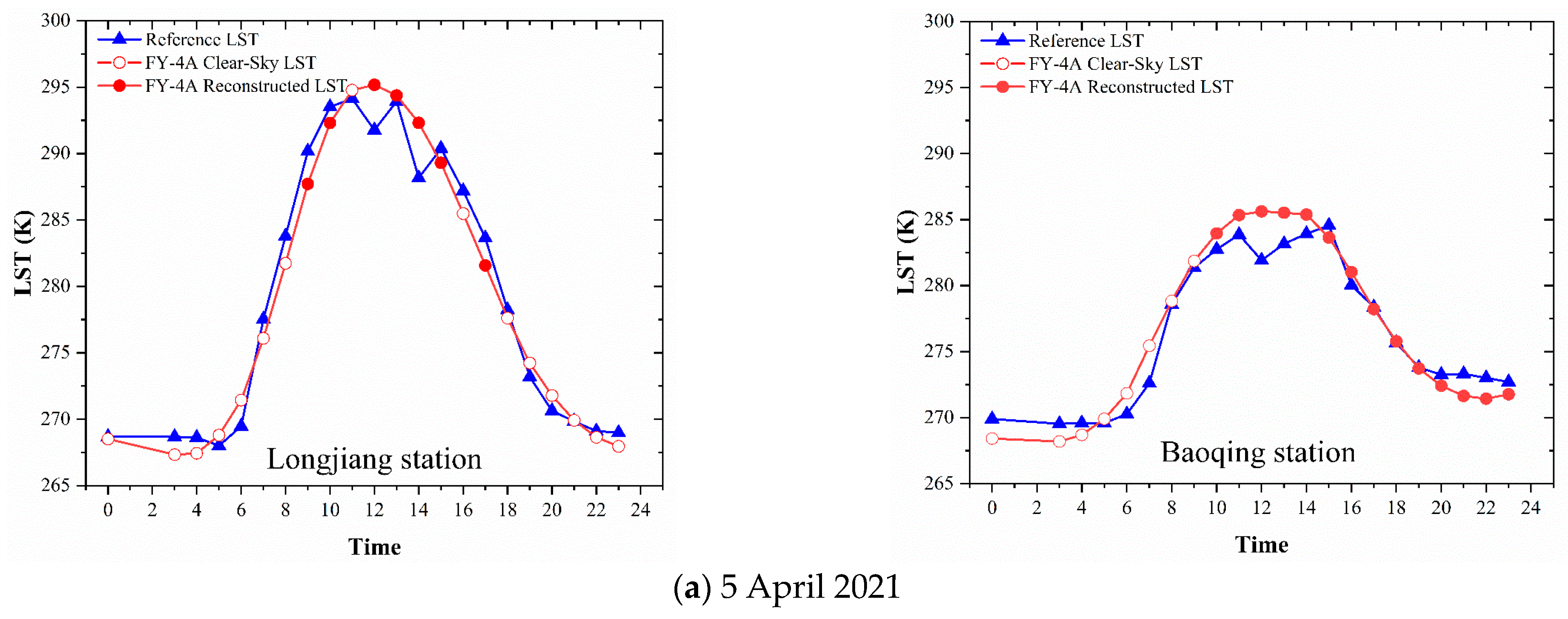
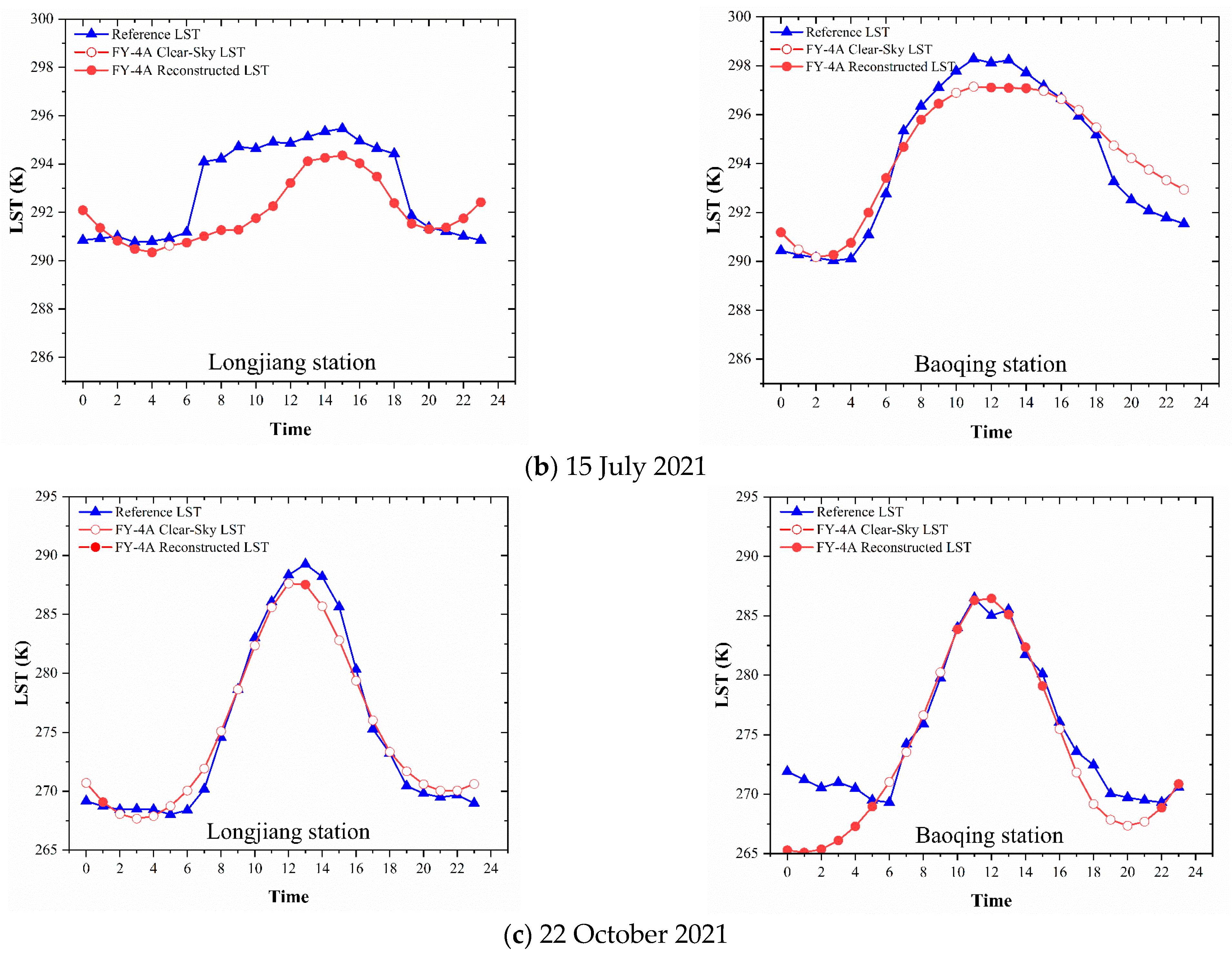
In addition, this study used the hourly measured LST of representative meteorological stations after scale conversion to form time series reference data, and compared them with the reconstructed LST of corresponding pixels in the temporal dimension. Taking Longjiang meteorological station (47.3°N, 123.2°E) and Baoqing meteorological station (46.4°N, 132.2°E) as examples, the time series of the reconstructed LST and the reference LST are shown in Figure 8.

It can be seen from Figure 8 that the reference LST of the selected two meteorological stations has a high similarity with the reconstructed LST in the temporal dimension, which can be explained as follows: (1) From 0:00 to 4:00, due to the surface upward long-wave radiation energy being greater than the atmospheric downward radiation energy, and the lack of solar short-wave radiation energy as a source of heat, the surface net radiation flux is negative, resulting in the LST generally showing a downward trend. (2) At 5:00, the sun gradually rises, and the surface begins to absorb solar short-wave radiation energy. The net radiation flux gradually changes from negative to positive, and the LST shows an upward trend. At about 13:00, the net radiation flux reaches the peak value, resulting in the LST reaching the maximum value. (3) After 14:00, the solar elevation angle gradually decreased, and the solar radiation energy absorbed by the surface gradually decreased. Meanwhile, the surface continued to radiate outward, and the LST showed a downward trend.

Moreover, the reconstructed LST appears to be temporally smoother than the reference LST. This phenomenon can be explained from both data and methodological perspectives. From a data standpoint, the reconstructed LST, which is derived from a larger scale of pixels, inherently captures a more generalized trend of LST, thus averaging out localized anomalies and microclimatic variations, leading to a temporal series that is less susceptible to the fluctuations that might be observed in station-specific measurements. On the methodological side, during the process of LST reconstruction, the S–G filtering method was implemented pixel-by-pixel in the temporal dimension to reduce the impact of noise and to address outliers. Abrupt increases or decreases of LST within individual time segments are mitigated through the application of S–G filtering.

4. Discussion

4.1. Advantages

The FY-4A AGRI LST products often contain blank areas due to cloud coverage. To address this problem, the study proposed a hybrid method for reconstructing the spatially and temporally continuous LST datasets of a geostationary meteorological satellite combining spatial and temporal information. The spatial distribution and the time series of the reconstructed LST shown in Figure 3 and Figure 8 indicate that the random forest regression algorithm has strong potential in capturing the relationship between LST and its predictor variables, and the proposed method can maintain the spatial and temporal variation trend in LST to the greatest extent. Moreover, the accuracy validation based on the reconstructed LST and the reference LST, measured by representative meteorological stations after scale correction, has proven that the results of the proposed method have a strong correlation with the reference LST, indicating that the results of the method are actual cloudy-sky LSTs.

The LST prediction data used in this study come from a variety of high-precision remote sensing data sources, which can be downloaded for free and are easy to obtain. The LST correlation model can be constructed using random forest regression to realize the fusion of multi-source remote sensing data. As shown in Figure 3, the proposed method has a robust performance when applied to FY-4A AGRI LST data of different times and seasons.

In addition, the study compared the proposed method with the method proposed by Zhao and Duan (2020) by applying these methods to reconstruct daytime LST on 5 April. As shown in Figure 5, both methods could recover the missing value of LST under cloud-covered conditions. Based on the visual comparison, the results of the two methods showed a similar trend of the LST in the spatial dimension. The LST reconstructed by SNR contains relatively less obvious abrupt points and boundaries than those reconstructed by DSSR. Moreover, the accuracy validation of the two methods shown in Figure 6 indicate that the reconstruction method proposed in this study has a relatively high accuracy. Therefore, the proposed hybrid method proved to have strong potential for recovering actual cloudy-sky LST. Moreover, due to the lack of solar radiation at night, the method proposed by Zhao and Duan can only apply to the daytime reconstruction of actual cloud-covered LST. In contrast, this study first introduced surface cumulative net radiation reanalysis data to describe the variation of LST throughout the whole day, therefore reconstructing hourly LST under cloud-covered conditions in high accuracy.

4.2. Limitations

Although the LST reconstruction model proposed in this study can achieve good results in the reconstruction of the missing values of cloud-covered pixels in all-day LST products, there are still some limitations in this method. First, because this model is based on the random forest regression algorithm, and the random forest regression algorithm is a machine learning model, the number and quality of training samples are required to be high. Therefore, it is difficult to use this method to construct an accurate LST correlation model for cases where a large area of cloud cover leads to a high missing rate of LST, which greatly affects the accuracy of the reconstruction results.

Secondly, there are many remote sensing data sources obtained in this study. The scale conversion process of different data sources is a simple bilinear interpolation resampling method for upscaling or downscaling, without considering the actual natural conditions of the surface, which may have a certain impact on the accuracy of the LST correlation model, thereby affecting the reconstruction accuracy of LST. Therefore, the scale conversion method between different data sources needs to be studied further. Moreover, the LST correlation model constructed based on the random forest regression algorithm is essentially a statistical model, and its physical laws are difficult to explain.

Finally, as for the verification method, this study uses the measured LST of the representative meteorological station as a reference and performs quality control. A simple linear correction method is used for the scale conversion of the measured LST of representative sites. Although the correction effect of this method shows satisfying results, it is difficult to ensure the applicability of this method to each moment. Therefore, the questions of how to find the appropriate validation data, and how to find the appropriate scale conversion method, remain to be studied further.

5. Conclusions

The coverage of clouds has great influence on the spatial and temporal continuity of FY-4A AGRI LST products, which limits the application of the products in scientific research, such as surface thermal environment monitoring. With this problem in mind, this study uses a variety of remote sensing data sources and proposes a hybrid method based on random forest regression algorithm and S–G filtering to reconstruct LST under cloud-covered conditions, which realizes the effective filling of the cloud-covered pixel missing values and restores the spatial and temporal continuity of FY-4A AGRI LST.

In this study, the method was applied and tested in three days of different seasons in the study area, and the accuracy was evaluated by using the measured LST of representative meteorological stations after scale conversion as a reference. The results showed that there was a strong correlation between the reconstructed LST and the reference LST, and high similarity in the changes in a single-day time series. Validation of the reconstructed LST revealed that the bias remained within the interval of −1.13 K to 0.39 K, the average MAE was 2.02 K, and the average RMSE was 2.62 K, which indicated that the overall performance of the method was satisfactory, and the reconstruction accuracy was reliable.

The hybrid model based on random forest regression algorithm and S–G filtering proposed in this paper successfully realized the reconstruction of FY-4A AGRI Land Surface Temperature products under cloud-covered conditions. The multi-source remote sensing data selected in this study are easily obtained and the model is easily implemented. The LST reconstruction results have spatial and temporal continuity and high accuracy. In the case of a certain number of clear-sky pixels for reconstruction model training, the LST reconstruction model proposed in this study can provide a new solution for filling the vacancy values of high temporal resolution Land Surface Temperature products.

References

1. Xian, G.; Shi, H.; Zhou, Q.; Auch, R.; Gallo, K.; Wu, Z.; Kolian, M. Monitoring and Characterizing Multi-Decadal Variations of Urban Thermal Condition Using Time-Series Thermal Remote Sensing and Dynamic Land Cover Data. Remote Sens. Environ. 2022, 269, 112803. [Google Scholar] [CrossRef]
2. Coolbaugh, M.F.; Kratt, C.; Fallacaro, A.; Calvin, W.M.; Taranik, J.V. Detection of Geothermal Anomalies Using Advanced Spaceborne Thermal Emission and Reflection Radiometer (ASTER) Thermal Infrared Images at Bradys Hot Springs, Nevada, USA. Remote Sens. Environ. 2007, 106, 350–359. [Google Scholar] [CrossRef]
3. Schroeder, W.; Oliva, P.; Giglio, L.; Csiszar, I.A. The New VIIRS 375 m Active Fire Detection Data Product: Algorithm Description and Initial Assessment. Remote Sens. Environ. 2014, 143, 85–96. [Google Scholar] [CrossRef]
4. Crow, W.T.; Kustas, W.P.; Prueger, J.H. Monitoring Root-Zone Soil Moisture through the Assimilation of a Thermal Remote Sensing-Based Soil Moisture Proxy into a Water Balance Model. Remote Sens. Environ. 2008, 112, 1268–1281. [Google Scholar] [CrossRef]
5. Chen, J.M.; Liu, J. Evolution of Evapotranspiration Models Using Thermal and Shortwave Remote Sensing Data. Remote Sens. Environ. 2020, 237, 111594. [Google Scholar] [CrossRef]
6. Yu, W.; Tan, J.; Ma, M.; Li, X.; She, X.; Song, Z. An Effective Similar-Pixel Reconstruction of the High-Frequency Cloud-Covered Areas of Southwest China. Remote Sen. 2019, 11, 336. [Google Scholar] [CrossRef]
7. Duan, S.-B.; Li, Z.-L.; Leng, P. A Framework for the Retrieval of All-Weather Land Surface Temperature at a High Spatial Resolution from Polar-Orbiting Thermal Infrared and Passive Microwave Data. Remote Sens. Environ. 2017, 195, 107–117. [Google Scholar] [CrossRef]
8. Zhang, X.; Zhou, J.; Göttsche, F.-M.; Zhan, W.; Liu, S.; Cao, R. A Method Based on Temporal Component Decomposition for Estimating 1-Km All-Weather Land Surface Temperature by Merging Satellite Thermal Infrared and Passive Microwave Observations. IEEE Trans. Geosci. Remote Sens. 2019, 57, 4670–4691. [Google Scholar] [CrossRef]
9. Wu, P.; Yin, Z.; Yang, H.; Wu, Y.; Ma, X. Reconstructing Geostationary Satellite Land Surface Temperature Imagery Based on a Multiscale Feature Connected Convolutional Neural Network. Remote Sens. 2019, 11, 300. [Google Scholar] [CrossRef]
10. Neteler, M. Estimating Daily Land Surface Temperatures in Mountainous Environments by Reconstructed MODIS LST Data. Remote Sens. 2010, 2, 333–351. [Google Scholar] [CrossRef]
11. Ke, L.; Ding, X.; Song, C. Reconstruction of Time-Series MODIS LST in Central Qinghai-Tibet Plateau Using Geostatistical Approach. IEEE Geosci. Remote Sens. Lett. 2013, 10, 1602–1606. [Google Scholar] [CrossRef]
12. Jia, A.; Ma, H.; Liang, S.; Wang, D. Cloudy-Sky Land Surface Temperature from VIIRS and MODIS Satellite Data Using a Surface Energy Balance-Based Method. Remote Sens. Environ. 2021, 263, 112566. [Google Scholar] [CrossRef]
13. Jin, M.; Dickinson, R.E. A Generalized Algorithm for Retrieving Cloudy Sky Skin Temperature from Satellite Thermal Infrared Radiances. J. Geophys. Res. Atmos. 2000, 105, 27037–27047. [Google Scholar] [CrossRef]
14. Das, M.; Ghosh, S.K. A Deep-Learning-Based Forecasting Ensemble to Predict Missing Data for Remote Sensing Analysis. IEEE J. Sel. Top. Appl. Earth Obs. Remote Sens. 2017, 10, 5228–5236. [Google Scholar] [CrossRef]
15. Zhang, Q.; Yuan, Q.; Zeng, C.; Li, X.; Wei, Y. Missing Data Reconstruction in Remote Sensing Image With a Unified Spatial–Temporal–Spectral Deep Convolutional Neural Network. IEEE Trans. Geosci. Remote Sens. 2018, 56, 4274–4288. [Google Scholar] [CrossRef]
16. Zhao, W.; Duan, S.-B. Reconstruction of Daytime Land Surface Temperatures under Cloud-Covered Conditions Using Integrated MODIS/Terra Land Products and MSG Geostationary Satellite Data. Remote Sens. Environ. 2020, 247, 111931. [Google Scholar] [CrossRef]
17. Parton, W.J.; Logan, J.A. A Model for Diurnal Variation in Soil and Air Temperature. Agric. Meteorol. 1981, 23, 205–216. [Google Scholar] [CrossRef]
18. Jin, M.; Dickinson, R.E. Interpolation of Surface Radiative Temperature Measured from Polar Orbiting Satellites to a Diurnal Cycle: 1. Without Clouds. J. Geophys. Res. Atmos. 1999, 104, 2105–2116. [Google Scholar] [CrossRef]
19. Jin, M. Interpolation of Surface Radiative Temperature Measured from Polar Orbiting Satellites to a Diurnal Cycle: 2. Cloudy-Pixel Treatment. J. Geophys. Res. Atmos. 2000, 105, 4061–4076. [Google Scholar] [CrossRef]
20. Fu, P.; Weng, Q. Consistent Land Surface Temperature Data Generation from Irregularly Spaced Landsat Imagery. Remote Sens. Environ. 2016, 184, 175–187. [Google Scholar] [CrossRef]
21. Huang, F.; Zhan, W.; Duan, S.-B.; Ju, W.; Quan, J. A Generic Framework for Modeling Diurnal Land Surface Temperatures with Remotely Sensed Thermal Observations under Clear Sky. Remote Sens. Environ. 2014, 150, 140–151. [Google Scholar] [CrossRef]
22. Wang, A.; Yang, Y.; Pan, X.; Hu, J. Land Surface Temperature Reconstruction Model of FY-4A Cloudy Pixels Considering Spatial and Temporal Characteristics. Geomat. Inf. Sci. Wuhan Univ. 2021, 46, 852–862. [Google Scholar] [CrossRef]
23. Ding, L.; Zhou, J.; Li, Z.-L.; Ma, J.; Shi, C.; Sun, S.; Wang, Z. Reconstruction of Hourly All-Weather Land Surface Temperature by Integrating Reanalysis Data and Thermal Infrared Data From Geostationary Satellites (RTG). IEEE Trans. Geosci. Remote Sens. 2022, 60, 5003917. [Google Scholar] [CrossRef]
24. Yang, J.; Huang, X. The 30 m Annual Land Cover Dataset and Its Dynamics in China from 1990 to 2019. Earth Syst. Sci. Data 2021, 13, 3907–3925. [Google Scholar] [CrossRef]
25. Jin, M.; Dickinson, R.E. Land Surface Skin Temperature Climatology: Benefitting from the Strengths of Satellite Observations. Environ. Res. Lett. 2010, 5, 044004. [Google Scholar] [CrossRef]
26. He, J.; Zhao, W.; Li, A.; Wen, F.; Yu, D. The Impact of the Terrain Effect on Land Surface Temperature Variation Based on Landsat-8 Observations in Mountainous Areas. Int. J. Remote Sens. 2019, 40, 1808–1827. [Google Scholar] [CrossRef]
27. Jia, A.; Liang, S.; Jiang, B.; Zhang, X.; Wang, G. Comprehensive Assessment of Global Surface Net Radiation Products and Uncertainty Analysis. J. Geophys. Res. Atmos. 2018, 123, 1970–1989. [Google Scholar] [CrossRef]
28. Copernicus Climate Change Service (C3S). C.C.C. C3S ERA5-Land Reanalysis. Copernic. Clim. Chang. Serv. 2019. [Google Scholar] [CrossRef]
29. Zhao, W.; Duan, S.-B.; Li, A.; Yin, G. A Practical Method for Reducing Terrain Effect on Land Surface Temperature Using Random Forest Regression. Remote Sens. Environ. 2019, 221, 635–649. [Google Scholar] [CrossRef]
30. Breiman, L. Random Forests. Mach. Learn. 2001, 45, 5–32. [Google Scholar] [CrossRef]
31. Belgiu, M.; Drăguţ, L. Random Forest in Remote Sensing: A Review of Applications and Future Directions. ISPRS J. Photogramm. Remote Sens. 2016, 114, 24–31. [Google Scholar] [CrossRef]
32. Savitzky, A.; Golay, M.J.E. Smoothing and Differentiation of Data by Simplified Least Squares Procedures. Anal. Chem. 1964, 36, 1627–1639. [Google Scholar] [CrossRef]
Figure 1. Land cover and elevation map of Heilongjiang Province, China.
Remotesensing 16 01777 g001
Figure 2. Flowchart of the proposed hybrid method for reconstruction of cloudy-sky Land Surface Temperature (LST).
Remotesensing 16 01777 g002
Figure 3. The original LST images and hourly reconstructed FY-4A AGRI LST on 5 April, 15 July and 22 October 2021, Heilongjiang Province, China.
Remotesensing 16 01777 g003
Figure 4. Random forest variable importance averaged of selected three days and their standard deviations. (15 April, 15 July, 22 October).
Remotesensing 16 01777 g004
Figure 5. The FY-4A AGRI LST images of Heilongjiang Province and the results of the reconstruction using two methods in the daytime of 5 April 2021.
Remotesensing 16 01777 g005
Figure 6. The validation of the reconstructed LST using two methods against the reference LST in the daytime of 5 April. Each point represents an hourly comparison between the reconstructed LST of FY-4A cloudy-sky pixel and the reference LST from the corresponding representative meteorological station in the daytime of 5 April. The red line represents the 1:1 line.
Remotesensing 16 01777 g006
Figure 7. Accuracy validation of the hourly reconstructed cloud-covered LST against reference LST measured by representative meteorological stations after scale correction on the selected three days. (5 April, 15 July, 22 October). Each point represents an hourly comparison between the reconstructed LST of FY-4A cloudy-sky pixel and the reference LST from the corresponding representative meteorological station on the specified dates. The red line represents the 1:1 line.
Remotesensing 16 01777 g007
Figure 8. The time series of the reconstructed LST and the reference LST of the selected two meteorological stations on the selected three days. (The FY-4A LST data at 1:00 and 2:00 (UTC+8) on 5 April were removed due to quality problems).
Remotesensing 16 01777 g008aRemotesensing 16 01777 g008b