1. Introduction
Microwave land surface emissivity (MLSE) is an important parameter that characterizes the radiative capability of the Earth’s surface, which is the ratio of thermal radiation emitted by the surface at a given temperature to the radiation emitted by a blackbody at the same temperature. It is influenced by surface characteristics and properties. In terms of describing surface features, satellite data assimilation, and retrieval, land surface emissivity is one of the key influencing factors. Therefore, it is of great significance to improve land surface emissivity retrieval.
The research on microwave land surface emissivity primarily focuses on its influencing factors and retrieval methods. Regarding the influencing factors, Norouzi et al. [
1] proposed that the difference in land surface emissivity originates from the influence of sensor parameters, surface, and subsurface by comparing different microwave land surface emissivity products. Xie et al. [
2] found that an uncertainty of 5–10% in land surface emissivity produces a brightness temperature uncertainty of about 5 K. When studying microwave land surface emissivity in desert areas, Guan et al. [
3,
4,
5] focused on its relationship with surface temperature, surface humidity, and soil moisture in the two subsurface layers, and built a land surface emissivity retrieval model based on the principle of radiative transfer and optimal control theory, which improved accuracy in simulating brightness temperature by the community radiative transfer model. All the above studies show that there are many factors affecting microwave land surface emissivity, and the selection of suitable influencing factors in suitable areas is an important condition for the accurate retrieval of microwave land surface emissivity.
Currently, several retrieval methods have been developed for microwave land surface emissivity estimation. Ferraro et al. [
6,
7] made a comparative study of the land surface model, direct observation, and the physical model in microwave land surface emissivity estimation and carried out a centralized quantitative evaluation. The physical models were estimated according to the physical relationships with soil surface variables such as soil moisture and surface roughness [
8]. These models include the classical Kirchhoff approximation model, small perturbation model, integral equation model, and advanced integral equation model [
9,
10,
11]. However, the physical models are difficult to directly apply to the retrieval of a large amount of data due to their complex construction and multiple input parameters.
In comparison, semi-empirical models are more suitable for practical applications. The most commonly used semi-empirical model is the Q/H model proposed by Wang [
12] and Choudhury [
13]. Based on the Q/H model, other semi-empirical models were developed by modifying roughness parameters, such as the
model [
14]. Shi et al. [
15] developed the
model based on the sensor configuration of the Advanced Microwave Scanning Radiometer for EOS (AMSR-E). The polarization dependence induced by surface roughness is considered. However, most of the currently available models rely on limited ground measurement conditions or discrete model formulations and are often limited in their application.
In recent years, due to the extensive use of machine learning, its advantages in the field of atmospheric science and numerical weather prediction have gradually emerged. To improve the visible infrared imaging radiometer derived surface products, Zhang et al. [
16] used machine learning algorithms to replace the original numerical retrieval scheme of the radiative transfer model to estimate multiple variables simultaneously, and the results were more accurate and effective compared to the existing satellite products. Aires et al. [
17] developed a neural network retrieval method to retrieve surface temperature, water vapor content, cloud liquid water paths, and microwave land surface emissivity from 19 GHz to 85 GHz over the land surface using the Special Sensor Microwave Imager observations, and their retrieval of microwave land surface emissivity more accurately reflected the gradients of vegetation and arid regions as well as specific hydrological structures. Chen et al. [
18,
19] combined the FY3C Microwave Radiation Imager sensor brightness temperature data with the community radiative transfer model, and utilized a neural network algorithm to perform a nonlinear retrieval of the microwave land surface emissivity in the desert region, whose retrieval accuracy was higher than that of the linear retrieval, but there is still room for improvement.
To sum up, the retrieval of microwave land surface emissivity in the current traditional model faces the problems of complex physical model construction, numerous input parameters, difficulty in directly applying to a large amount of data, and high dependence on ground measurement conditions, while the application of machine learning in this area is still shallow, considering that machine learning algorithms have the following advantages in the retrieval process of land surface emissivity: (1) ability of nonlinear modeling; (2) adaptive and flexible; (3) large-scale data processing capabilities, etc. Therefore, in order to further improve the retrieval accuracy of microwave land surface emissivity, other machine learning algorithms will be used in this paper.
3. Retrieval Model Establishment
According to the optimal control theory, combined with the simulated brightness temperature and the observed brightness temperature, a cost function
J is constructed:
where the subscript “2” represents the L-2 norm, and the superscript “2” represents the square of the L-2 norm.
represents the observed brightness temperature from FY3C Microwave Radiation Imager-I,
represents the simulated brightness temperature from the community radiative transfer model,
ε represents the microwave land surface emissivity, and
X represents the input variables for the forward simulation in the community radiative transfer model.
Microwave land surface emissivity is a factor that is influenced by multiple environmental variables. It can be seen as a function of the influencing factors, denoted as:
where
represents surface temperature,
represents surface humidity, and
represent soil moisture at 0.07 m and 0.28 m below the surface, respectively [
4]. In order to find the relational equation of function
g, three models are established using four influence factors. The first is the optimized Bayesian regularized neural network retrieval model (M2_30NN) on the basis of the original neural network retrieval model (M1_20NN) [
19]. The second and third are the random forest retrieval model (RF) and the extreme gradient boosting tree retrieval model (XGBoost).
As a result, we have built different microwave land surface emissivity retrieval g-functions using three models. However, it is not only the microwave land surface emissivity alone that affects the output of the community radiative transfer model simulated brightness temperature, but also various other related variables. The ultimate goal of this paper is to improve the accuracy of the land surface emissivity and optimize the output of the community radiative transfer model simulated brightness temperature, so after obtaining the g-function, we do not consider the individual deviation of the g-function itself, but introduce the land surface emissivity obtained from the g-function into the community radiative transfer model, and comprehensively consider the common deviation of the two. The g-function with the optimal common deviation is used as the optimal land surface emissivity improvement model, where the criterion to be considered is the comparison of the simulated brightness temperature of the land surface emissivity obtained from the g-function with the satellite-observed brightness temperature.
The choice of random forest and extreme gradient boosting tree algorithms to study the problem is based on the following aspects: (1) both the random forest and XGBoost algorithms are integrated learning methods based on decision trees, which are excellent in dealing with high-dimensional, nonlinear problems, and they are able to automatically capture the complex relationship between the input features and generate accurate prediction results; (2) the random forest and XGBoost algorithms are robust to missing data and noise, it can effectively reduce the risk of overfitting. The XGBoost algorithm can also effectively control the complexity of the model and improve the generalization ability of the model; (3) the random forest and XGBoost algorithms have high computational efficiency when dealing with large-scale data. In addition, we have also conducted a comparison of the advantages and disadvantages among algorithms using single-day data, including support vector machine, linear regression, random forest, and XGBoost, and the results show that the random forest and XGBoost algorithms have a better retrieval ability for this problem.
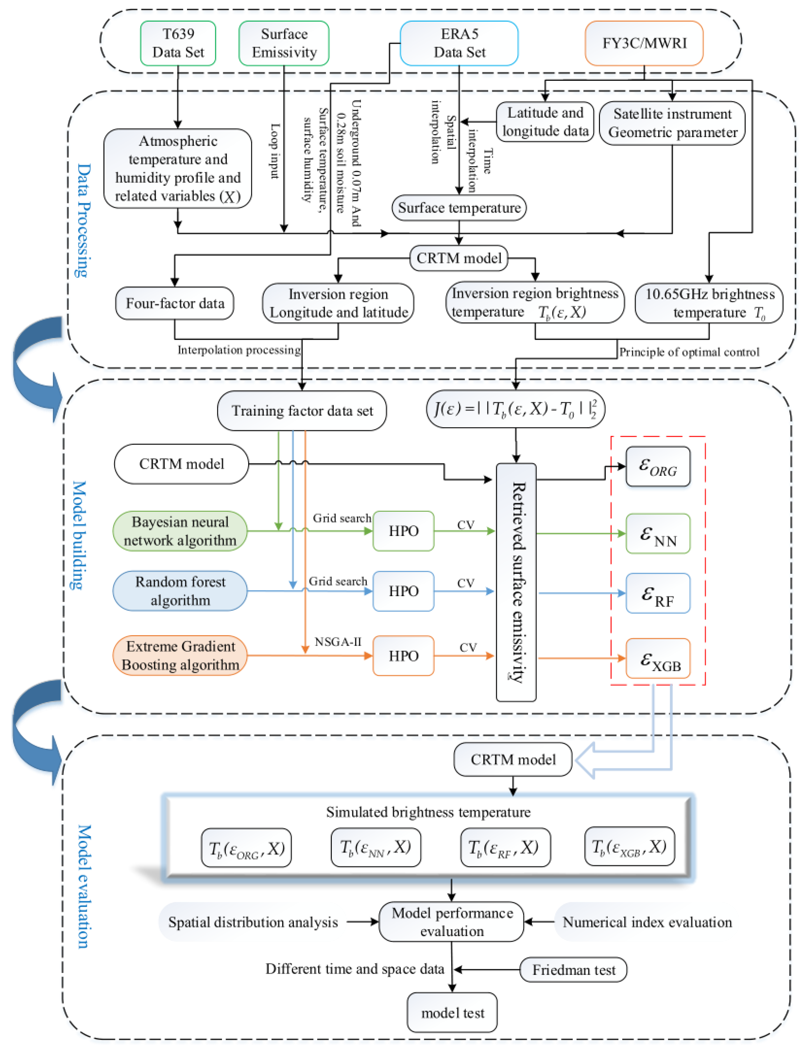
The main project of this thesis is broadly divided into three parts: data processing, model building, and model evaluation. In the data processing part, we obtain the atmospheric temperature and humidity profiles and related variables by running the T639 model, which is used as the boundary input of the community radiative transfer model; we download the satellite-observed brightness temperature data from the relevant websites; we extract the four-factor variables from the Fifth-Generation European Re-Analysis dataset, and obtain the training dataset and the related data after temporal interpolation and inverse distance weighted interpolation, which are used for the model construction. In the second part, different algorithms are preliminarily evaluated to determine the retrieval scheme, and the preliminarily established model is continuously optimized and improved according to the optimal control principle scheme to finally obtain the land surface emissivity close to the observed brightness temperature state. In the third part, we add the retrieved land surface emissivity into the community radiative transfer model, run the community radiative transfer model, and analyze and test the simulated brightness temperature with the observed brightness temperature to verify its reliability.
Figure 2 shows the specific technical roadmap of this study.
3.1. Neural Network Model
In order to further optimize the retrieval model for microwave land surface emissivity, a Bayesian regularization backpropagation neural network method is chosen. This is a combination of Bayesian inference and BP neural networks for dealing with overfitting in neural networks.
For a neural network model, it can be viewed as a probabilistic model, i.e., a conditional distribution model : Input x, output predicted y distribution, w is the weight in the neural network. When the research problem is a classification problem, y is a set of categories, and the conditional probability distribution corresponds to the probabilities of each category; when the research problem is a regression task, y is , and is Gaussian, corresponding to the squared loss. The weights w can be learned by maximum likelihood estimation (MLE), based on the gradient descent method. Regularization is performed by placing a prior on the weights w and finding the maximum posterior weights . If w is given a Gaussian prior, this produces L2 regularization (or weight decay, with a tendency to take small values). If w is given a Laplace prior, then the L1 regularization is recovered (with a tendency to take 0 and sparse weights).
The basic idea of Bayesian regularization is to introduce a regularization term into the loss function of the neural network to constrain the values of the model parameters. Bayesian inference for neural networks is computed as the posterior distribution of
weights given the training datasets, which predicts the value of the unknown data by taking the expectation:
Each possible weight configuration is weighted according to the posterior distribution, and predictions are made for the unknown labels of the given test data item. Monte Carlo approximation and local reparameterization of the objective function are performed according to the theories proposed by Charles et al. [
23] and Diederik et al. [
24], respectively, to finally obtain the network.
Wang et al. [
19] carried out the retrieval of microwave land surface emissivity based on Bayesian regularized neural network, optimized the hyperparameters in the network in terms of the number of hidden layers (1, 2, 3) and the number of nodes in the hidden layers (10, 20, 30, 40, 50), respectively, and got the optimal hyperparameter setting of the whole winter microwave land surface emissivity retrieval model as 1 hidden layer and 20 nodes in the hidden layer, That is, the M1_20NN model.
Improving parameters such as the number of hidden layers, the number of hidden layer nodes, and the activation function of a neural network can have a significant impact on the performance and learning ability of the network. Increasing the number of hidden layers can increase the hierarchical structure of the network, and deeper networks can capture higher-level features through layer-by-layer abstraction, thus improving the network’s expressive and generalization capabilities; increasing the number of hidden layer nodes can increase the capacity of the network so that it can represent more complex functional relationships, thus improving the network’s fitting ability; the activation function introduces nonlinearities into the neural network, and it is key to realizing the nonlinear transformation, and different activation functions have different properties and nonlinear characteristics.
Therefore, in this study, based on the M1_20NN model, a grid search is performed to automatically rank different combinations of these three aspects based on the loss function. Cross-validation is also employed to prevent overfitting and improve the reliability of the model. These result in the development of the retrieval model M2_30NN. The scope of the grid search is specified in
Table 1.
3.2. Random Forest Model
Random forest (RF) is a tree predictor combination algorithm proposed by Breiman [
25] in 2001. Each tree used in RF relies on a random vector value, which is independently sampled and has the same distribution for all trees in the forest. RF is an ensemble learning method that generates multiple different training sets by randomly sampling from the original sample set. Subsequently, each training dataset is modeled separately, and the output results of all models are combined to obtain the final prediction.
Figure 3 illustrates the flowchart for retrieving microwave land surface emissivity using the random forest algorithm.
Random forest is a powerful and popular machine learning algorithm. Compared with other algorithms, it has the following advantages: (1) Robustness: Since it is an integrated model based on multiple decision trees, overfitting of a single tree will not have much impact on the overall model; (2) Scalability: Random forest can process datasets with hundreds or even thousands of features, performing well on high-dimensional data and large-scale data without dimensionality reduction; (3) It is not easy to overfit: by randomly selecting feature subsets and sample subsets to build each tree, random forest effectively reduces the risk of overfitting. In general, random forests perform well in situations where they handle complex data, have many features, and require high accuracy and robustness, so they are widely used in practical applications.
Therefore, random forest is selected as one of the retrieval schemes in this paper. For the RF retrieval model, the hyperparameters (number of decision trees, maximum number of features, maximum depth of the decision tree, minimum number of samples to be considered when splitting a node, minimum number of samples required for a leaf node) are selected using grid search (GridSearchCV), and 10-fold cross-validation is added to evaluate the generalization error of the learner. The specific hyperparameter optimization ranges are shown in
Table 2.
3.3. Extreme Gradient Boosting Model
The extreme gradient boosting tree algorithm (XGBoost) is a machine learning system based on gradient boosting [
26]. XGBoost utilizes a tree-integrated model, which consists of a group of classification and regression trees (CARTs). This type of tree-based learning is known as tree boosting. Because one tree may not be sufficient to achieve good results, multiple classification and regression trees can be used at the same time, and the final prediction is the sum of each Classification and Regression Tree score. The model can be represented as:
where
f is a function of the function space
, and
represents the sets of all possible classification and regression trees. Here,
q represents the mapping of an example to the corresponding leaf indices in each tree structure,
T denotes the number of leaves in a tree,
w represents the leaf weights, and
k indicates the number of trees. The objective to optimize can be expressed as:
The training is performed in an additive manner by adding terms , which helps minimize the objective. Here, represents the prediction of instance i at iteration t − 1, is the training loss function, and is the regularization term.
XGBoost is a gradient boosting tree algorithm. Compared with other algorithms, it has the following advantages: (1) High accuracy: XGBoost performs well on many datasets. It uses the gradient boosting algorithm and combines the advantages of the decision tree model, which can effectively improve the accuracy of the prediction; (2) Parallel processing: XGBoost is able to automatically make use of multi-core processors to perform parallel computation so that the training on large-scale datasets faster; (3) Flexibility: XGBoost supports custom optimization objectives and evaluation criteria, which can meet a variety of different types of machine learning tasks. So, we choose XGBoost as another retrieval scheme.
To obtain an optimized model adapted to the microwave land surface emissivity retrieval problem, the Non-Dominated Sorting Genetic Algorithms II (NSGA-II) [
27,
28] is introduced to tune the relevant parameters of XGBoost. The four-factor variables of ERA5 are taken as input data, and the crossover, variation, and selection of genetic algorithms are used to optimize the XGBoost decision tree quantity, maximum depth of decision tree, learning rate, sampling proportion of training samples of each tree and sampling proportion of features of each tree during training, and the optimal parameter combination is screened independently. The optimal microwave land surface emissivity retrieval model is obtained by selecting the optimal combination according to the results of non-dominated ordering, and the model is trained and tested.
The Non-Dominated Sorting Genetic Algorithms II algorithm is introduced in order to achieve automatic screening of the model for hyperparameters and to obtain the optimal solution. The specific operation of this algorithm is shown below:
- (1)
Randomly generate an initial population of size , which undergoes non-dominated sorting, selection, crossover, and mutation to produce a progeny population , and unite the two populations to form a population of size ;
- (2)
Perform fast non-dominated sorting, calculate the crowding degree of individuals in each non-dominated layer at the same time, and select suitable individuals to form a new parent population according to the non-dominated relationship and the crowding degree of individuals;
- (3)
Generate a new offspring population through the basic operations of the genetic algorithm, merge and to form a new population , and repeat the above operations until the conditions for the end of the procedure are met.
4. Experimental Design and Result Analysis
4.1. Experimental Design
To retrieve winter microwave land surface emissivity, training datasets are selected from December 2014 to January 2019, specifically encompassing the months of December, January, and February. The specific training dates and the dates for independent validation are provided in
Table 3.
The ERA5 surface temperature, surface humidity, and soil moisture of 0.07 m and 0.28 m underground are used as independent variables. The objective is to minimize the error between the simulated brightness temperature from the retrieved microwave land surface emissivity and the observed brightness temperature, which corresponds to minimizing the cost function (2). Training is performed using each retrieval model, resulting in the M2_30NN retrieval model, the RF retrieval model, and the XGBoost retrieval model for microwave land surface emissivity, respectively. Finally, the microwave land surface emissivity obtained from each retrieval model is used to simulate the brightness temperature using the community radiative transfer model, and the simulated brightness temperatures from each model are analyzed and compared.
4.2. Analysis of Model Training Results
The collected data consists of 49 days with a total of 31,8376 samples, of which we set 80% as training data and the rest as testing. Taking the observed bright temperature as a reference, the performance evaluation indexes can be obtained by calculating the simulated bright temperature of each retrieval model: the simulated brightness temperature of the RF retrieval model shows the best performance in various indexes, and its correlation coefficient with the observed brightness temperature reaches 0.9116, which is 14.21% higher than that of the original model of 0.7982. In addition, the root mean square error of the simulated and observed brightness temperatures of the RF retrieval model is 3.1802 K, and the mean absolute error is 1.1942 K, which, respectively, represent a 38.71% and 66.47% improvement over the original model. In contrast, the XGBoost retrieval model performs less favorably. The M1_20NN retrieval model shows slight improvement over the original model, with a correlation coefficient of 0.8455, representing a 5.92% improvement, but significantly lower than the improvements seen in the RF and XGBoost retrieval models. Unfortunately, the improved M2_30NN model, despite the hyperparameter changes, performs the worst in terms of simulated brightness temperature results after applying it to the community radiative transfer model. Looking at the explained variance of residual sum for each retrieval model, the reliability of the RF and XGBoost retrieval models improved from 57.53% in the original model to 82.89% and 81.25%, respectively, with both representing an improvement of more than 40%. On the other hand, the M1_20NN and M2_30NN retrieval models only showed an improvement of around 20%.
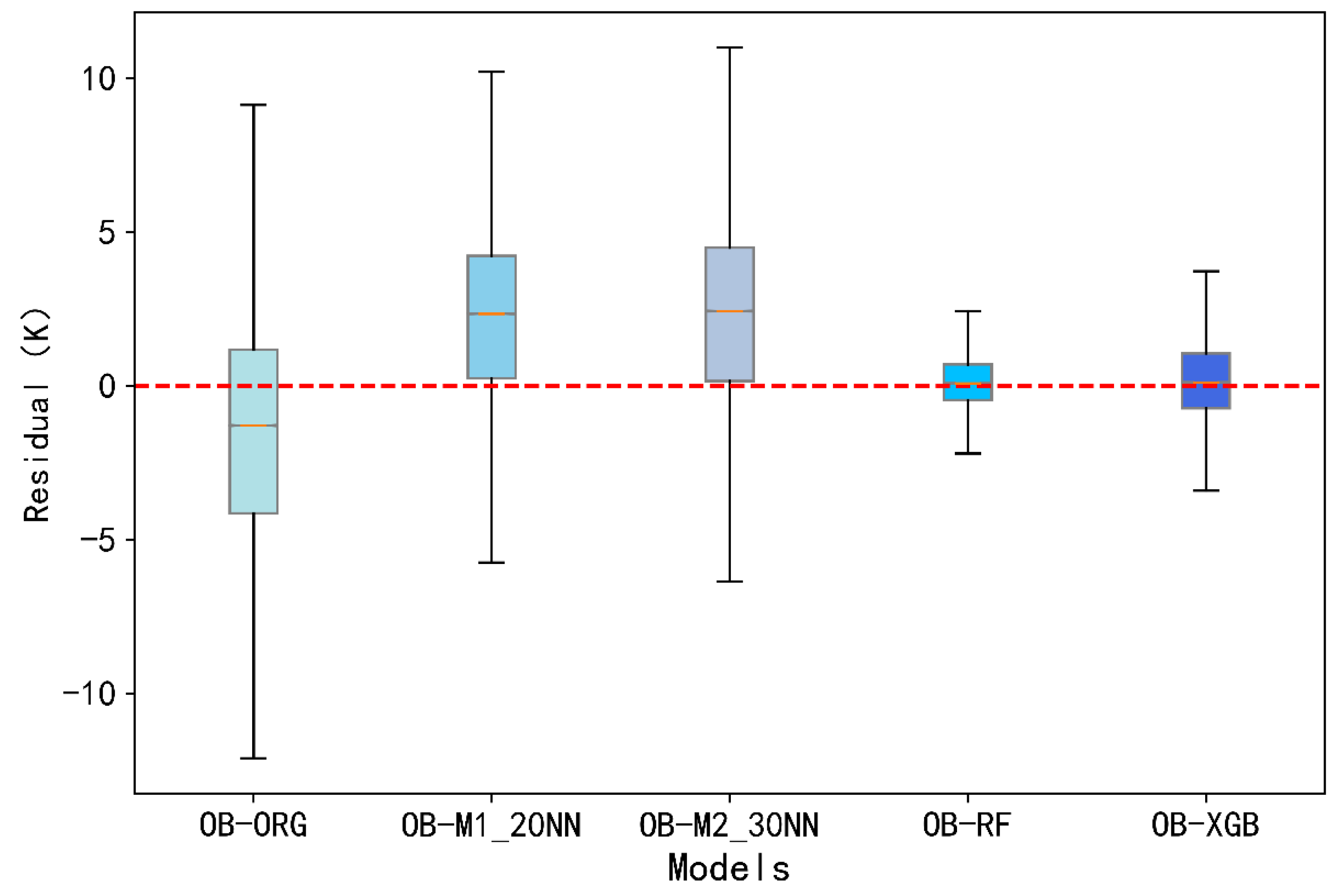
Figure 4 shows the difference between the simulated and observed brightness temperatures based on the different retrieval models, and it can be seen that the original community radiative transfer model simulates the brightness temperature in the region poorly, with a wide range of residual distributions; the neural-network-based land surface emissivity retrieval model underestimates the regional brightness temperatures, and the degree of dispersion is only second to that of the original model; and the integrated-tree-based RF and XGBoost land surface emissivity retrieval models simulate a more concentrated distribution of brightness temperatures (around 0) with a small degree of dispersion, which is in very good agreement with the observations.
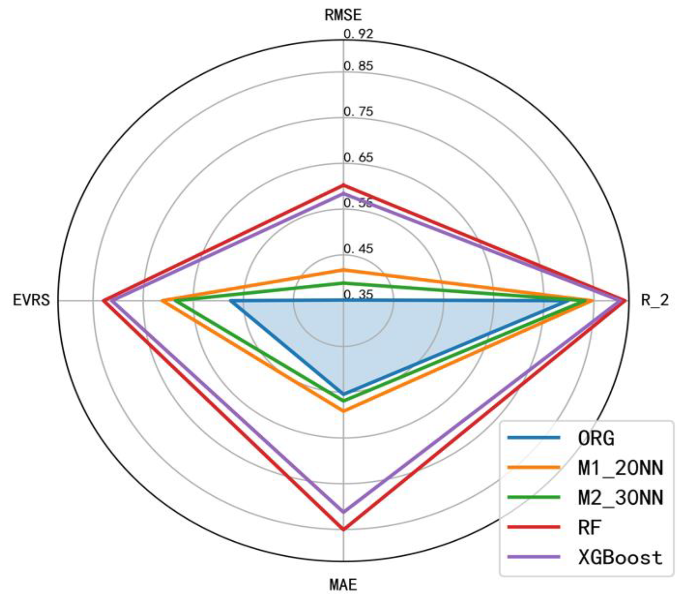
The radar chart obtained from the root mean square error and mean absolute error calculations, combining the Pearson correlation coefficient and the explained variance of residual sum are shown in
Figure 5. Therefore, the larger the area of the quadrilateral formed by each retrieval model in the radar chart, the better. The shaded region represents the statistical indicator results of the simulated brightness temperature from the original community radiative transfer model compared to the observed brightness temperature. From
Figure 5, it can be shown that the performance of the retrieval models, from high to low, is as follows:
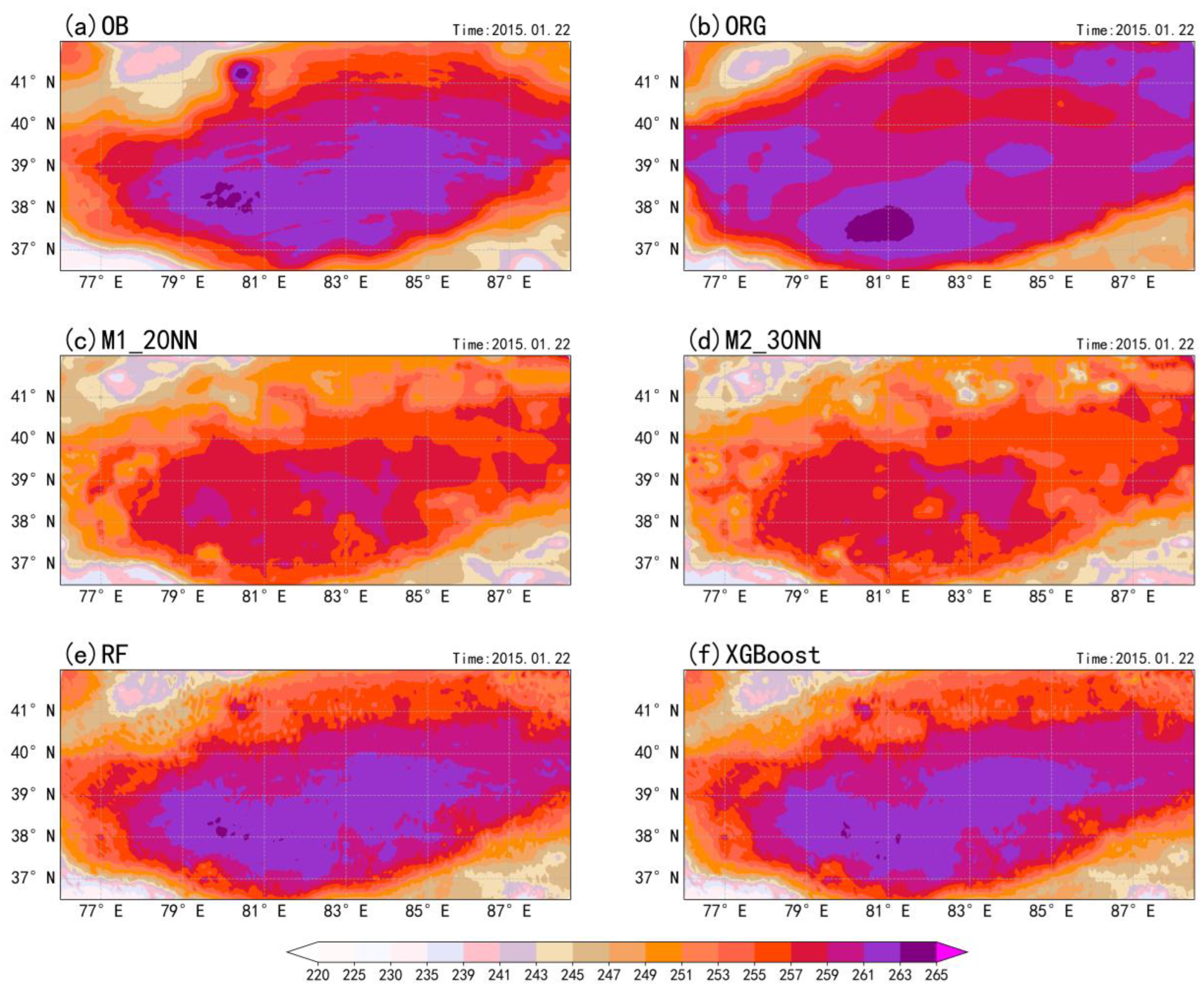
For a more comprehensive evaluation of the training results of the retrieval models,
Figure 6 is the spatial distribution of brightness temperature on 22 January 2015. From
Figure 6a, it can be seen that the observed brightness temperature in the Taklamakan Desert region exhibits higher values, which gradually decrease outward from the high-value areas, coinciding with the high surface temperatures in desert regions. There is also a high-value center located at approximately 71.5°E and 41°N. However, the original simulated brightness temperature based on the community radiative transfer model shows a wider range of high values and overestimates the brightness temperature in some desert areas (
Figure 6b). This large error is also evident from the plot of the difference between simulated and observed brightness temperature (
Figure 7a). In
Figure 6c,d, the high-value regions of the simulated brightness temperature based on neural network methods for microwave land surface emissivity retrieval appear scattered and lower compared to the observations. On the other hand, the RF and XGBoost models successfully capture the distribution pattern of the observed brightness temperature and simulate the high-value center in the northern region (
Figure 6e,f), showing a closer resemblance to the observations.
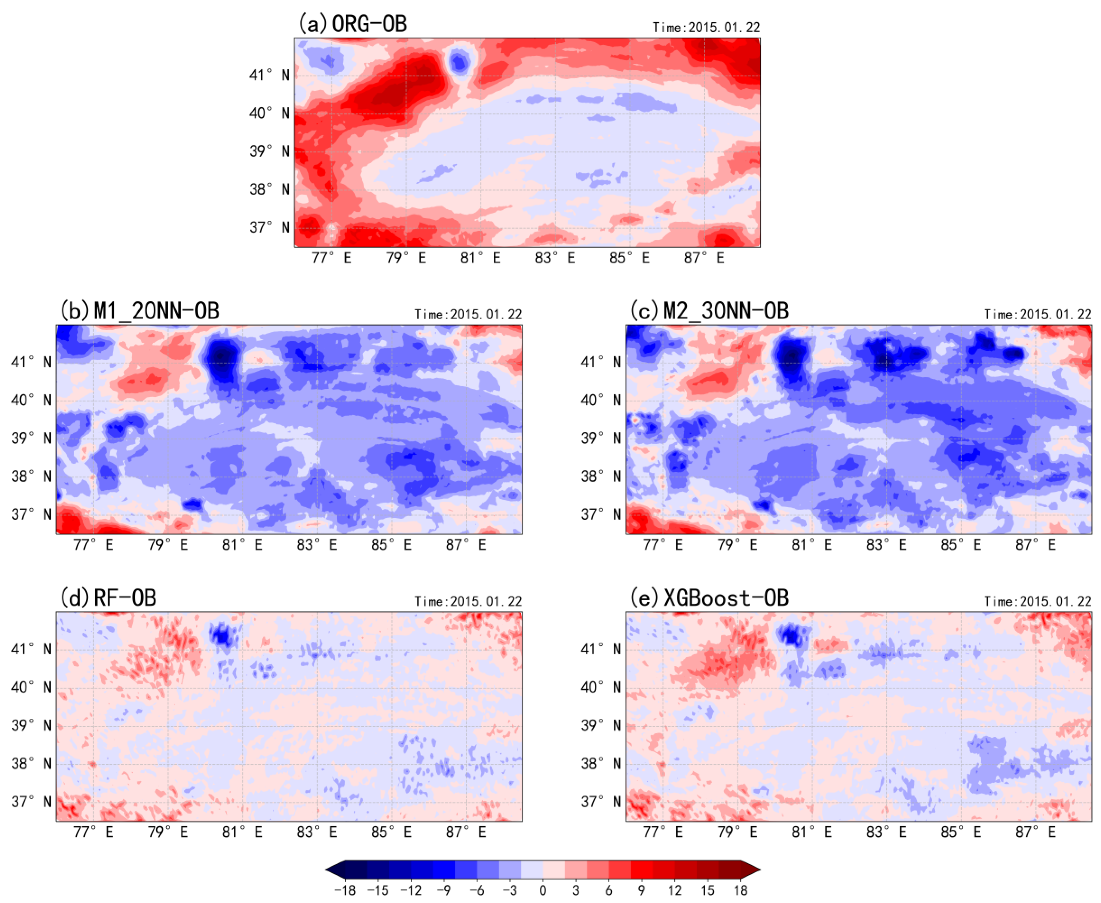
Figure 7 represents the difference between the simulated brightness temperatures of the retrieved microwave land surface emissivity from each model and the observed brightness temperatures. As can be seen in
Figure 7a, the simulated brightness temperature of the original microwave land surface emissivity in the community radiative transfer model is poorly simulated at the edge of the desert, and there is a general overestimation phenomenon, and in
Figure 7b,c, the difference between the simulated brightness temperature of the retrieved microwave land surface emissivity of the model and the observed brightness temperature ranges from −9 K to −4 K, and the distribution of the error in the northernmost part of the desert exceeds even −9 K. However, in
Figure 7d,e, the distribution of differences is more uniform and significantly reduced, ranging roughly from −2 K to +2 K. Therefore, the RF and XGBoost models perform better in microwave land surface emissivity retrieval across the entire Taklamakan Desert, as evidenced by the RMSE and MAE falling between 0.9 K and 1.8 K.
4.3. Model Evaluation
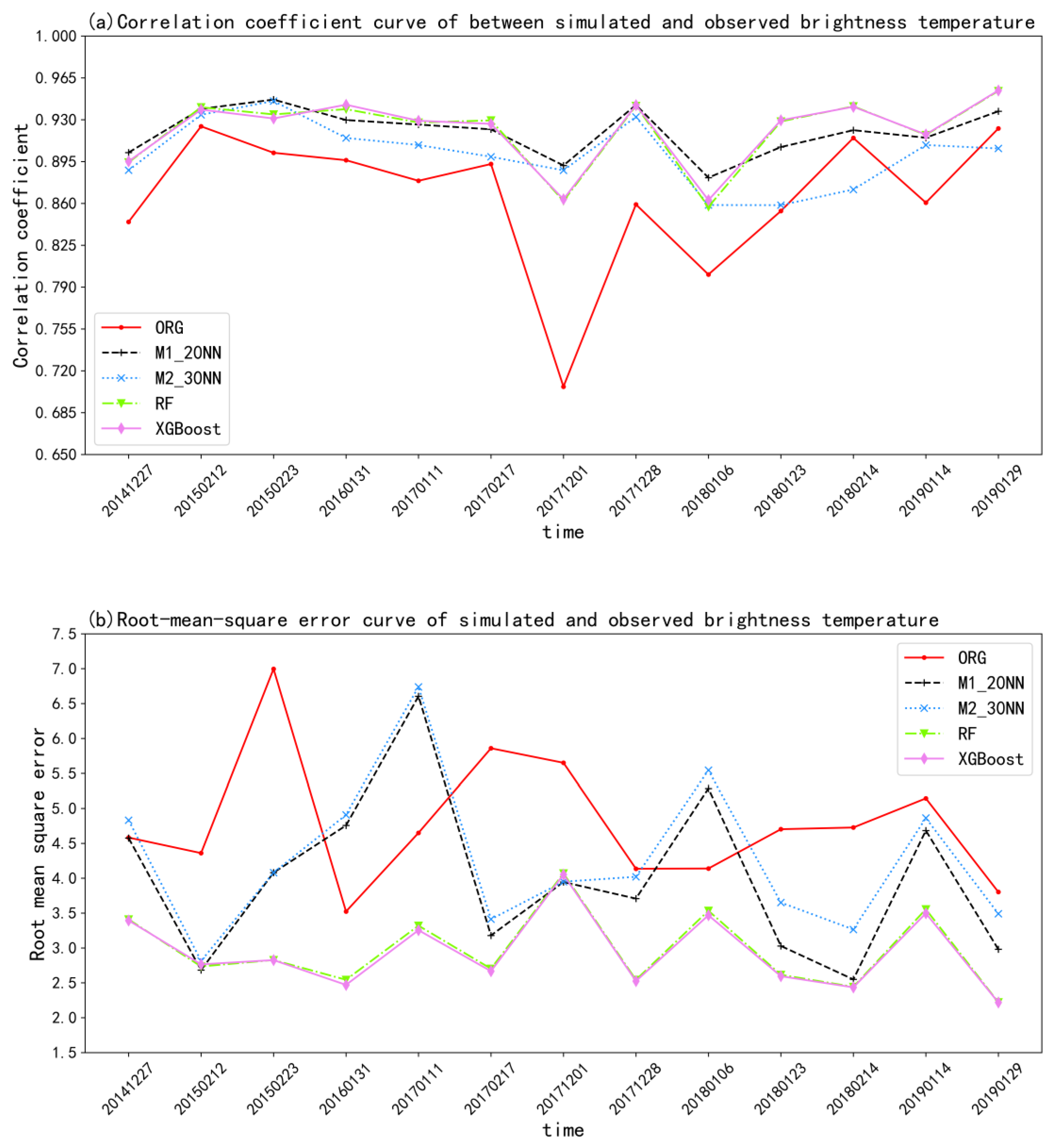
To evaluate the generalization ability and comprehensive ranking of independent samples in the model,
Figure 8 presents the root mean square error and correlation coefficient of the simulated brightness temperature of microwave land surface emissivity obtained by each retrieval model in 13 independent verification datasets.
As can be seen from the change curve of correlation coefficient between simulated brightness temperature of microwave land surface emissivity retrieval by the improved machine learning models and observed brightness temperature (
Figure 8a), the simulated brightness temperature of microwave land surface emissivity retrieved by the improved machine learning models is also closer to the observation in the test datasets than that simulated by the original community radiative transfer model, and changes under different dates are more stable than that simulated by the original community radiative transfer model.
Notably, both the XGBoost model (pink curve) and the RF model (green curve) not only exhibit higher correlation coefficients than the neural-network-based M1_20NN and M2_30NN models in the training set but also demonstrate outstanding performance in the test datasets.
Figure 8b displays the root mean square error variations between the simulated brightness temperatures of the retrieved microwave land surface emissivity from each model and the observed brightness temperatures. It can be observed that the RF model and the XGBoost model have relatively lower root mean square error values with smaller fluctuation trends, oscillating around 3 K. However, the M1_20NN and M2_30NN models exhibit larger variation ranges and lower accuracy, oscillating between 2.5 K and 7 K.
To further compare the performance of each retrieval model on the test datasets, we conducted a Friedman test [
29,
30] by calculating the average ranking of each model. This test aims to examine whether all models have similar performance on the test datasets, with the null hypothesis stating that “the performance of the retrieval models is the same”. The ranking is first determined based on the weighted average of the Pearson correlation coefficient, root mean square error, mean absolute error, and explained variance of residual sum of the simulated and observed brightness temperatures of the microwave land surface emissivity of each retrieval model in the test datasets, the results are shown in
Table 4.
By applying the principles of the Friedman test, the test statistic is calculated, which is 18.06. It follows an F-distribution with degrees of freedom (3, 36), and the critical value is 2.565. Therefore, the null hypothesis is rejected, indicating that the performance of the retrieval models significantly differs.
Considering the average rankings after comprehensive sorting, the XGBoost retrieval model demonstrates the best performance on the evaluation dates, followed by the RF retrieval model.
5. Conclusions and Discussion
For the retrieval of microwave land surface emissivity, three optimized retrieval models, namely M2_30NN, RF, and XGBoost, were developed by introducing machine learning algorithms based on the original M1_20NN retrieval model. The models were trained using four land surface emissivity influence factor data for 49 winter days and validated using a further 13 days of four-factor data. The results obtained are as follows:
- (1)
In the training datasets, the RF retrieval model performs better in terms of overall performance compared to the other three retrieval models. The XGBoost retrieval model has a slightly lower performance than RF. Although M1_20NN and M2_30NN also show some performance improvements, they cannot describe the distribution pattern of observed brightness temperature very well;
- (2)
According to the evaluation of cross-validation t-tests, the p-values between each pair of the four retrieval models are all less than 0.05, indicating that there are significant performance differences among the retrieval models;
- (3)
In terms of evaluation on test datasets, the XGBoost retrieval model demonstrates better generalization capabilities than RF. Both retrieval models are able to simulate the distribution pattern of brightness temperature well, and they show stability in the retrieval results of microwave land surface emissivity throughout the winter season. The performance of the M1_20NN and M2_30NN retrieval models also show some improvement compared to the original community radiative transfer model, but it is significantly lower than the other two models and exhibits larger fluctuations and instability during the winter season. In the Friedman test, there are significant differences in the performance of all algorithms. Based on the average rank ordering, the generalization capabilities on test datasets are as follows:
Interestingly, in the training datasets, the RF retrieval model performed the best, followed by XGBoost. However, there is a slight variation in the results when it comes to the testing datasets, with the XGBoost retrieval model performing the best, followed by RF.
For XGBoost, the principle is an improvement of the gradient boosting algorithm, which uses Newton’s method when solving for the extremes of the loss function, Taylor expansion of the loss function to the second order, and additionally, a regularization term is added to the loss function. RF, on the other hand, uses a decision tree as a base classifier, constructing multiple decision trees by randomly selecting subsets of features and samples, and classifying or regressing by voting or averaging the predicted results. In analyzing the above occurrences, it is explained in the following ways [
31,
32]:
- (1)
Overfitting: random forests overfit the noise and details of the training samples on the training set, leading to a performance degradation on the test dataset. In contrast, XGBoost uses a gradient boosting algorithm, which makes it easier to prevent overfitting by controlling the model’s complexity and regularization, it is easier to prevent overfitting;
- (2)
Data imbalance: the retrieval model built in this paper selects four factors that affect the land surface emissivity, and some decision trees may not have enough opportunities to learn the features of rare categories, which affects the performance on the test dataset. In contrast, XGBoost can better handle the sample imbalance problem by adjusting the sample weights through parameters or using other methods to deal with unbalanced data;
- (3)
Parameter tuning: XGBoost has more parameters that can be tuned, and by optimizing these parameters, it is possible to control the complexity and effectiveness of the model more precisely in order to train the model for the better. For random forests, the choice of parameters is simpler because each decision tree is generated independently and does not have parameters that usually need to be tuned.
In conclusion, the M2_30NN, RF, and XGBoost retrieval models for microwave land surface emissivity are established by optimizing the M1_20NN retrieval model and introducing the random forest and extreme gradient boosting tree algorithm. The RF and XGBoost retrieval models demonstrate the best performance on the training datasets, testing datasets, and generalization ability. This significantly improves the accuracy of microwave land surface emissivity retrieval in the Taklamakan Desert region.


 and
and 

