Abstract
Building ecological networks can effectively enhance the quality and stability of ecosystems and better conserve biodiversity. Previous studies mainly determined ecological corridors based on selecting ecological sources at a regional scale (e.g., an administrative area), without considering the bioclimatic heterogeneity within the study area. Here, we propose a novel integrating approach involving bioclimatic zoning and selecting ecological sources from various bioclimatic zones to design ecological corridors. Taking Xi’an City, China, as an example, key bioclimatic variables were first chosen, and we partitioned the study area based on its bioclimatic characteristics through a combination of K-means clustering and variance inflation factor (VIF). Ecological sources were then identified from the combination of ecosystem services and habitats of 36 endangered species. Subsequently, the minimum cumulative resistance (MCR) model was used to build ecological networks within different bioclimatic zones and across the entire region. We found the following: (1) In Xi’an city, a total of 49 source areas and 117 corridors were identified. The identified network can protect 97.77% of species, facilitating connectivity between 30.50% of ecosystems and 35.5% of species-rich areas. (2) The integrating approach protects 12.26% more species richness and 10.95% more ecosystem services than the average value of the regional and bioregional approaches. Compared to regional and bioregional methods, integrating approaches demonstrate greater advantages in preserving species richness and ecosystem services. This study introduces a novel approach to constructing regional ecological networks, which integrates the impact of bioclimatic zoning into the process of network construction to improve ecosystem services and protect species habitats.
1. Introduction
The intricacy of global biodiversity conservation challenges has escalated due to the intricate interplay between, factors like habitat loss, climate change, and socio-economic pressures [1,2,3]. The establishment of protected areas has been adopted as a good strategy to solve this problem and has been supported and implemented in many countries [4,5,6,7,8]. However, the effectiveness of the protected area system has proven inadequate in mitigating the pace of biodiversity loss [9,10], largely due to limitations in terms of size, ecological representation, and governance [7]. Compared to individual protected areas, ecological networks show greater advantages in connecting populations, maintaining ecosystem function, and protecting biodiversity [11]. Safeguarding ecological networks not only mitigates habitat fragmentation but also establishes vital connections among isolated protected areas within a cohesive and interconnected system [12].
Concepts similar to ecological networks include urban infrastructure (GI) and ecological security pattern (ESP). They differ in their different focuses; GI focuses on urban environmental conditions and citizens’ health and quality of life [13,14], while ESP focuses more on the sustainability of ecosystem functions and services [15,16,17]. The ecological network is a comprehensive framework comprising core habitats (often called ecological sources which contain protected areas, other effective areas, and undisturbed natural areas), connected through ecological corridors [6]. This network is intentionally established, restored, and maintained to ensure the protection of biological diversity within fragmented ecosystems. The theory of landscape ecology is used to identify ecological networks, and the fundamental research paradigm of “ecological source-ecological corridor” has been introduced and widely embraced as a method for identifying ENs [11,18]. In this paradigm, one of the critical prerequisites for building ecological corridors and networks is to build ecological sources. The process of selecting ecological sources is influenced by the objectives of ecological networks construction, resulting in diverse criteria. These different criteria focus on various aspects, such as biodiversity preservation [19,20], climate mitigation [21,22], or ecosystem services [23]. However, the concurrent assessment of both biodiversity and ecosystem services remains relatively limited, especially in terms of analyzing biodiversity using species occurrence data. Another important part is the construction of the ecological resistance surface. Making an ecological resistance surface, which characterizes barriers in biological migration, is a crucial prerequisite for developing an ecological network. Many scholars construct ecological resistance surfaces based on variables of land use and human interference [24,25,26]. Although various studies have considered multiple factors and made adjustments to ecological resistance surfaces, there is no widespread consensus on the calculation of ecological resistance surfaces [27]. In addition, the minimum cumulative resistance (MCR) model, ant algorithm, and circuit theory can be used comprehensively to realize the effective extraction of ecological corridors and ecological networks [26,28,29].
There are a significant number of studies on ecological networks, which have been researched at different scales, encompassing global [18,24,30], national [31,32,33], and regional levels [34]. Previous studies mainly focused on identifying ecological networks across an entire region, such as an entire administrative area. However, inadequate consideration has been given to the impact of extension changes. Owing to the considerable spatial heterogeneity in the distribution of ecosystem functioning and biodiversity, the ecological corridors resulting from the selection of ecological sources across the entire study area tend to cluster within specific sub-regions, rather than effectively linking diverse and heterogeneous sub-regions. Although there is a study based on regional and interregional approaches to construct ecological corridors for eliminating the influence of spatial heterogeneity, it considers administrative extension rather than biological extension. Ecological networks are important to protect ecological diversity and promote ecosystem service flows, so it is very important to analyze the impact of ecological corridors and ecological networks from the perspective of the species.
The distribution of different animals and plants on the surface of the Earth is uneven as a result of the interaction between historical and ecological variables, and the geographical features of the land itself are obstructed, resulting in the formation of several bioclimate divisions [35]. Regional climate and environmental conditions differ due to regional differences, while climate and temperature are similar in a given bioclimatic zone [36]. The species within the bioclimate zone are relatively the same, and the migration activities of the same species are within this specific zone. For these reasons, we used bioclimatic zoning to explore the impact of extension changes from a biological perspective. However, at larger scales, such as the national and global levels, research on its impact can obtain broader and more objective results. Research at the regional scale, especially in areas with obvious regional heterogeneity, can more effectively support the practical implementation activities of ecological networks and ecological corridors construction.
The current analysis filled the research gap in several ways. Firstly, we calculated a variety of ecosystem services and calculated species richness using the maximum entropy model. Second, we used bioclimatic factors to partition the study area and explored the impact of extension on the construction of ecological corridors. Finally, we proposed a method for integrating biological preferences to construct ecological networks, and compared it with traditional methods.
2. Material and Methods
2.1. Study Area
Xi’an City is located on the north–south border of Shaanxi Province in China, in the Huaihe River line of the Qinling Mountains. The Qin-Huaihe line serves as the natural boundary between northern and southern China. The Qin-Huaihe line includes the Qinling Mountains, which are located south of Xi’an. With significant variances in regional climate and terrain, Xi’an’s topography is high in the north and low in the south. A significant population resides north of the Huaihe River line, whereas the Qinling Mountains’ greenery is more abundant south of the Huaihe River line. Xi’an city belongs to the warm temperate semi-humid monsoon climate, with an annual average temperature of 6.4–13.4 °C and an annual average precipitation of 537.5–1028.4 mm. This region serves as a crucial transitional zone for flora and fauna, making it a representative area for global biodiversity. According to the “First Survey Report on Wildlife Resources in Xi’an”, there are 548 species of terrestrial vertebrates belonging to 32 orders and 110 families in Xi’an, including 13 species listed as first-class nationally protected wildlife and 56 species as second-class nationally protected wildlife. The Qinling Mountains serve as the habitat for threatened and rare species such as giant pandas (Ailuropoda melanoleuca), takins (Budorcas taxicolor bedfordi), and golden snub-nosed monkeys (Rhinopithecus roxellana), highlighting the paramount importance of the region in maintaining biodiversity. In addition, there are various types of natural vegetation in the territory, mainly distributed in the Qinling Mountains in the south of Xi’an city, and succeeding with the change in altitude. The stark contrast between the north and the south of Xi’an gives rise to a diverse natural landscape and biodiversity, making it an ideal location for implementing ecological corridors based on bioclimatic divisions (Figure 1).
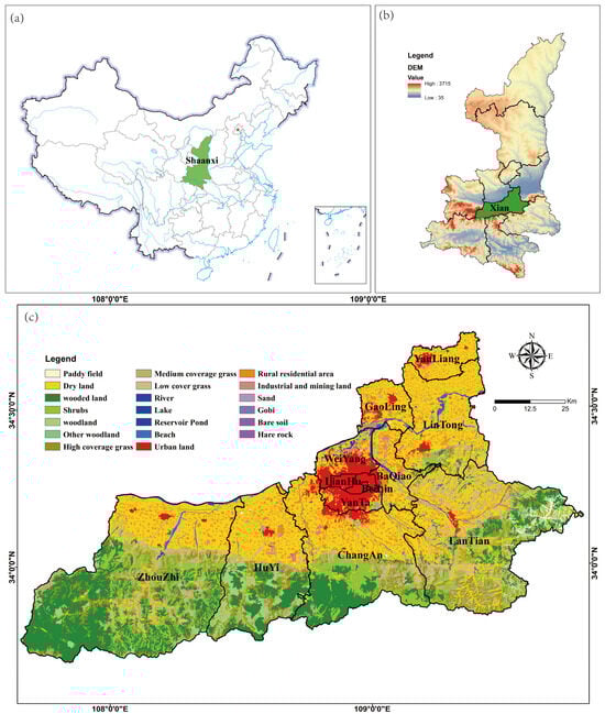
Figure 1.
Location map of Xi’an. (a) Shaanxi province is located in China. (b) Xi’an city is in Shaanxi province. (c) Land utilization in Xi’an.
2.2. Data Sources
Nineteen bioclimatic factors come from the WorldClim global climate database (http://worldclim.org/, accessed on 26 October 2022), and the resolution of the data is 1000 m. The specific explanation of bioclimatic factors is shown in Table 1; DEM uses the global primary geographic data digital elevation model NASA DEM provided by the National Aeronautics and Space Administration (NASA), and the resolution of the data is 30 m; HFI (human interference factors) come from NASA socio-economic Data and Application Center (SEDAC), and the resolution of the data is 1 km (https://sedac.ciesin.columbia.edu/, accessed on 31 October 2022) [37]; soil data come from the global soil grid information provided by the World Soil Information Center, and the resolution of the data is 250 m (https://www.isric.org/explore/soilgrids, accessed on 26 October 2022). The runoff data are provided by Geographic remote sensing ecological network platform (www.gisrs.cn, accessed on 11 August 2022). Precipitation data and evapotranspiration data come from the TerraClimate dataset (www.climatologylab.org, accessed on 10 August 2022); the normalized difference vegetation index data (Normalized Difference Vegetation Index, NDVI) come from the MOD13Q1 V6 product, and the resolution of the data is 250 m; the species data come from the “Xi’an Forestry Bureau’s Report on the Results of the First Wildlife Resources Survey Project in Xi’an City,” and integrate the published literature which records the distribution information data of essential species in Xi’an City, and simulate the habitats of a total of 36 crucial species (containing first- and second-level protected species); net primary productivity data (NPP) come from MODIS MOD17A3HGF V6 products, and the resolution of the data is 500 m.

Table 1.
Bioclimatic factors.
2.3. Ecosystem Services and Species Richness Assessment
According to the natural background of the study area and previous research [38], species richness and three vital ecosystem services (water conservation, soil conservation, and carbon sequestration) were considered and assessed in Xi’an City. The evaluation of these three ecosystem services was conducted from the years 2000 to 2020. We used the average values over this 20-year period as the basis for our assessment. The assessment results were divided into five levels based on the equal area method in ArcGIS10.8, i.e., lowest, low, medium, high, and highest.
2.3.1. Water Conservation
Water conservation is an important ecosystem service for regional development and ecological environment protection [39]. On an instantaneous scale, water conservation is achieved through vegetation canopy and litter interception, soil water storage and infiltration, runoff, and evapotranspiration processes. On an interannual scale, interception and water storage are ultimately exported to the ecosystem through evapotranspiration and runoff, that is, “water balance.” This study calculates water conservation by the water balance method [40], and the calculation formula is as follows:
In the formula, Q is water conservation (), P is rainfall (), SR is surface runoff (), ET is evapotranspiration (), and A is area (m2). Among them, rainfall and evaporation data come from the TerraClimate dataset, and runoff data come from the Geographic remote sensing ecological network platform.
2.3.2. Soil Conservation
The soil conservation service function is evaluated using the Revised Universal Soil Loss Equation (RUSLE) [26,41,42,43]. The calculation formula is as follows:
In the formula, is the average annual soil conservation amount (), is the average potential annual soil erosion, is the average actual annual soil erosion (), is the precipitation and runoff erosivity factor (), is the soil erodibility factor (, is the terrain factor (dimensionless, where is the slope length factor and is the slope factor), is the vegetation coverage and management factor (dimensionless), and is the factor of water and soil protection measures (dimensionless). Data sources for the study include precipitation data to calculate R from the TerraClimate dataset, NDVI to calculate C derived from the MOD13Q1 V6 product, DEM to calculate LS from the National Aeronautics and Space Administration, and soil characteristics to calculate K such as sand, clay, silt, and organic carbon data sourced from the World Soil Information Center.
2.3.3. Carbon Sequestration
Carbon fixation refers to the transformation of inorganic carbon into organic compounds by living organisms during photosynthesis [44]. The ecosystem’s net primary productivity (NPP) is quantified using the process-based CASA model. This model posits that plant productivity correlates with the photosynthetically active radiation absorbed or intercepted by green leaves [45]. NPP is chosen as a metric to characterize the carbon sequestration function of the ecosystem [46,47], and the unit of NPP is expressed in grams per square meter (g/m2).
2.3.4. Species Richness
The MaxEnt (Maximum Entropy) model is a species distribution model based on the maximum entropy theory. By training the species occurrence data and combining the environmental variables of the area where the species is located, each species habitat suitability can be predicted [48,49,50,51]. The environmental variables contain 19 bioclimatic factors, encompassing a range of variables such as temperature and rainfall, the detailed explanation of which can be seen in Table 1. According to the relevant literature [48], we divided each species‘ occurrences using 75% of the data for model calibration and retained 25% of the data for evaluation. We converted the probability of habitat suitability to binary outputs of habitat and non-habitat using the optimal threshold of maximum sensitivity and specificity [52]. Habitat is set to 1, non-habitat is set to 0, and the results of habitat simulation of 36 species are added up to obtain species richness.
2.4. Bioclimatic Division
Bioclimatic factors, DEM and HFI, were used for bioclimatic partitioning. We used VIF and k-means to check for the multicollinearity of the adjustment factors and determine the number of biotope divisions. The VIF has been used in many studies to remove collinearity between elements [53,54], and VIF > 5 indicates that there is a potential multicollinearity problem in the dataset [55]. When calculating the VIF, the evaluation factor with the highest VIF value is gradually eliminated until the VIF values of the remaining evaluation factors are all less than 5. Then, the k-means algorithm is used to evaluate the optimal number of classes to determine the optimal number of types [56,57]. Through the R4.2.2 platform, this paper uses the k-means function to realize the spatial clustering of bioclimatic factor clustering.
The 21 factors were analyzed with VIF analysis, and finally, five factors were screened out, namely BIO3, BIO4, BIO14, DEM, and HFI. The explanation of the specific factors is shown in Table 1. Among these factors, BIO3, BIO4, BIO14, and HFI are all grids of 1 km × 1 km, and the DEM is resampled into a grid of 1 km × 1 km. The values of the five factors corresponding to each 1 km × 1 km grid unit are extracted, and this is used for cluster analysis. As shown in Figure S1, the value of the graph tends to be flat when the category is equal to 3 and 4. After comparing the results of multiple clusters and combining them with the actual situation in Xi’an, we finally divide it into three categories. We process the results of the partitions, discard those of the same type but with a small area, integrate the aggregated ones, and finally delineate the partitions (Figure S2).
2.5. Ecological Sources Identification
Ecological sources are habitat patches that are crucial for regional ecological security because they play a significant role in regional ecological processes and functions and provide powerful radiative functions [58]. The four components were subjected to a multi-factor collinearity study using the VIF, and we discovered that no collinearity existed for any of their values below 5. Given that each ecosystem service is equally significant in Xi’an City, we employed standardization to establish a consistent range for ecosystem services, thereby eliminating any dimensional discrepancies. Ecological source identification mainly includes two parts: (1) Identification of ecological sources using a regional or bioregional approach. The regional method involves extracting the top 20% of ecologically significant areas within the entire study area, while also proposing patches with an area of less than 1 km2 as ecological sources. The bioregional method involves extracting the top 20% ecologically significant areas for ecosystem services in each bioclimatic zone, while also extracting patches with an area smaller than 1 km2 as ecological sources. (2) The implementation of an integrating approach will encompass the ecological sources identified through both the regional and bioregional approaches. The perspective of the regional method focuses solely on the highest-level ecosystem services and species richness within the entire region, but overlooks the influence of climate zoning on organisms. The identified ecological sources tend to concentrate in specific areas in regions with significant climate variations, particularly in Xi’an with distinct heterogeneity. As a result, the constructed ecological networks are limited to these specific zones, rendering the effect of the ecological networks constrained for the entire region. On the other hand, the bioregional approach takes into account bioclimatic zoning, leading to the distribution of source locations across various regions within the study area. However, this approach falls short in covering the most critical ecosystem services and species richness within the regional context. By combining these two methods, not only can comprehensive protection be achieved across the entire region, but the focus can also be maintained on the most important ecosystem services and species richness within the specific regional context.
2.6. Ecological Corridor Identify
The construction of ecological corridors can maintain ecosystem functions, reduce the fragmentation of ecological sources, and improve the connectivity of ecological sources [59]. The premise of building an ecological corridor is the need to build an ecological resistance surface. In this study, we adopt the definition of ecological resistance surfaces and refer to relevant research [39], using the InVEST habitat quality module to simulate the ecological resistance surface (see the Supplementary Materials in the Materials and Methods Section to construct resistance surfaces). This research uses the MCR model to construct ecological corridors. It is calculated as follows:
In the formula, is the minimum cumulative resistance value of ecological source patch j spreading to a certain point; is the spatial distance of base i that species cross from ecological source j to a certain point in space; is the impact of patch i on the ecological process or resistance to species movement.
Key ecological sources are defined as zones that overlap with ecological sources by regional and bioregional approaches. General ecological sources are defined as areas that do not overlap with ecological sources based on regional identification. Ecological corridors are built using the MCR model, which divides the links between different ecological sources into separate ecological corridors.
The ecological corridors were divided into key, general, and fragile corridors based on the connections before key ecological sources, connections between key ecological sources and general ecological sources, and connections before general ecological sources.
3. Results
3.1. Species Richness and Major Ecology Services
In Xi’an, there are considerable differences between the north and the south in the distribution of ecosystem services. Figure 2a shows the spatial pattern of the species richness in Xi’an City. The spatial distribution of high species richness patches (i.e., high and highest levels) is relatively scattered, mainly located at the east of Xi’an. The proportions of high species richness patches in Zhouzhi County, Huyi County, and Changan County are higher than in other counties (i.e., 59.76%, 56.67%, and 34.04%, respectively).
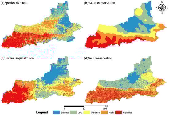
Figure 2.
Spatial patterns of ecosystem service and species richness in Xi’an.
The spatial pattern of water conservation importance is shown in Figure 2b. The ability to conserve water in Xi’an City’s northern region is the lowest, while the city’s core regions—primarily Zhouzhi, Huyi, and Changan District—show poor levels of water conservation. The districts of Zhouzhi, Huyi, and Changan have the high and highest proportions of carbon sequestration (73.34%, 49.47%, and 35.39%, respectively).
The spatial pattern of carbon sequestration importance is shown in Figure 2c. The capacity for carbon sequestration in Xi’an City’s eastern region is the lowest, and the city’s center regions, which are primarily spread across Xingchen District, Weiyang District, Beilin District, and Lianhu District, exhibit low-level carbon sequestration. The Zhouzhi, Lantian, and Huyi districts have the high and highest proportions of carbon sequestration (94.39%, 36.43%, and 26.30%, respectively).
The spatial pattern of soil conservation in Xi’an municipality is shown in Figure 2d. The high-quality patches (i.e., high and highest levels) in Zhouzhi County, Huyi County, and Lantian County account for high area proportions, accounting for 63.42%, 47.69%, and 41.40% of the total area of these cities, respectively, according to statistics on the soil conservation at different levels in eleven cities and each administrative area in Xi’an City. High-quality soil conservation patches are primarily found in the south of Xi’an; they are located in the Qinling Nature Reserve, where many laws and regulations prohibiting construction and conserving nature have been implemented, as opposed to the north, where the population is concentrated. However, there are no high-quality patches to be found in the Xingchen District, Weiyang District, Beilin District, or Lianhu District in the city center.
3.2. Bioclimatic Division
The research area is divided into three sub-regions (Zone I, Zone II, and Zone III) based on bioclimatic factors, with areas of 4882.59 km2, 550.20 km2, and 4666.01 km2, respectively (Figure 3a). As shown in Figure 1 and Figure S3, Zone I is mainly concentrated in the north of Xi’an, the sub-center of Xi’an, and the agricultural planting area. Zone II is primarily the urban construction area of Xi’an, and humans occupy a dominant position in this ecosystem. Zone III is mainly the Qinling Mountains in Xi’an City. This area is a crucial area of nature reserves in Xi’an.
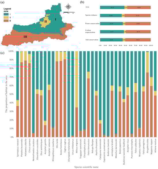
Figure 3.
Xi’an bioclimatic division map. (a) Bioclimatic zoning pattern map. (b) The proportion of species richness and major ecology services in different zones. (c) The proportion of each species’ predicted habitat area in different regions.
The proportions of the area occupied by different zones within the various partitions are not uniform across the total area. The area proportion of Zone I reaches 48.36%, while the proportion of Zone I accounts for only 5.45%. Although larger areas typically correlate with higher ecosystem service values and species richness, variations exist in the proportions of different ecosystem services or species richness values relative to the area (Figure 3b). As shown in Figure 3b, even though Zone III constitutes merely 46.2% of the total area, its value in terms of species richness, water resource conservation, soil preservation, and carbon sequestration surpasses its area proportion. In contrast, despite Zone I covering 48.35% of the area, its proportions of total area values related to species richness, water resource conservation, carbon sequestration, and soil preservation are 42.88%, 45.09%, 46.97%, and 44.85%, respectively. These proportions are lower than their area proportion, underscoring the disparities between area proportions and their corresponding values.
We simulated the distribution of 36 protected species in Xi’an using the Maxent model and delineated their habitats within the region. As shown in Figure 3c, we quantified the proportion of habitat in each zone relative to the total habitat. It is evident from the graph that the habitats of almost all species are primarily concentrated in Zones I and III. Furthermore, we observed that the primary habitats of 19 protected species are located in Zone III (where the proportion of habitat in Zone III exceeds that in Zones II and I). We infer that these species are mainly situated in Zone III, and the same logic applies to the subsequent discussion. Additionally, the primary habitats of 16 protected species are found in Zone II. In Zone I, which is predominantly utilized for urban development, only the habitat of the Black Kite (Milvus migrans) is primarily situated.
3.3. Spatial Distribution of Ecological Sources
The southern region of Xi’an is where the majority of the ecological sources are concentrated in contiguous areas by the regional approach. We found 16 ecological sources with a total area of 1893.28 km2, of which the most giant patch had an area of 1846.25 km2, occupying 97.52% of the total area of all ecological sources (Figure 4a). The bioregional approach identified a total of 108 ecological sources, distributed as 23, 10, and 75 sources in Zones I, II, and III, respectively. These source locations are distributed across various regions of Xi’an, with a higher concentration in the central and southern parts, while the northern region of Xi’an has notably fewer source locations. Using this methodology, the cumulative area of identified ecological sources amounted to 1661.04 km2. The largest single ecological source covered 657.19 km2, representing 39.56% of the total area of all ecological sources (Figure 4b). The integrated approach revealed 49 ecological sources covering a combined area of 2875.81 km2. On average, each ecological source had an area of 58.69 km2 (Figure 4c).
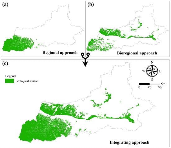
Figure 4.
Ecological sources distribution map. (a) The result of identifying ecological sources based on the whole domain (regional approach). (b) Results of identifying ecological sources by bioclimatic partitions (bioregion approach). (c) Ecological sources are determined through an integrating approach (integrating approach). The colored area represents the ecological source, and the colorless area represents the non-ecological source.
In general, considering these three methods, their proportional representation in terms of area is roughly similar to the proportion of corresponding species richness and ecosystem service value they can cover in the entire region. For instance, the area proportion for the regional approach is 21.62%, while within this region, the proportion of species diversity and ecosystem service value falls within the range of [20.89%, 23.43%]. Furthermore, despite the similarities in proportions, there are still some differences among the different methods. Taking the regional approach as an example, the coverage area proportion of this method is lower than the proportions for water conservation, soil conservation, and carbon sequestration across the coverage region. However, the situation is slightly different for the bioregional approach, wherein only the proportions for water conservation and carbon sequestration are lower than the overall area proportion. Across the three methods, the proportion of species richness in the entire region is higher than the proportion of coverage area (Figure 5).
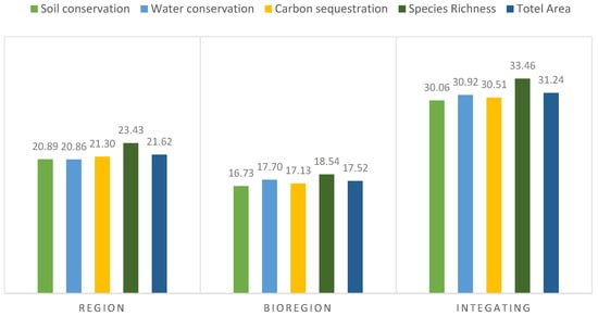
Figure 5.
The proportion of species richness and major ecology services in different methods.
3.4. Spatial Distribution of Ecological Corridors
Using the InVEST habitat quality model, the ecological resistance surface is built (see the Supplementary Materials for details). The ecological resistance surface of Xi’an exhibits lower resistance in the southern region and higher resistance in the northern region (Figure S4). The range of resistance values is from 0 to 97.82, with higher values indicating greater resistance. Within the study area, the average resistance value of individual pixels is 46.87. Areas with higher ecological resistance are primarily concentrated in urban centers and rural residential zones, with more human activity disturbance.
By combining the ecological sources identified through regional and bioregional methods, we obtained the ecological sources within the integrating approach. Using the MCR method, ecological corridors were successfully generated by integrating ecological sources and ecological resistance surfaces. Through this approach, a total of 49 ecological source areas and 117 ecological corridors were identified. Among these, there were a total of 34 key source areas, with an average area of 118.33 km2, primarily distributed in the southern region. In contrast, general source areas had an average area of 29.78 km2, predominantly scattered across the northern region (Figure 6).
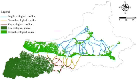
Figure 6.
Spatial pattern of ecological corridors.
In the identified ecological corridors, the general corridors had the highest count, while the fragile corridors had the lowest count, with 81 and 12, respectively. Key corridors, general corridors, and fragile corridors were distributed in the southern, central, and northern parts of the study area, respectively (Figure 6). Fragile corridors exhibited the highest average resistance value of 51.19, surpassing the overall average resistance value of the study area (46.87). Notably, this value also exceeded the sum of the average resistance values of general corridors (14.11) and key corridors (16.58). An increase in the average resistance value of corridors indicates decreased vulnerability and feasibility for development. Compared to key and general corridors, fragile corridors had lower feasibility for development.
4. Discussion
4.1. Comparison of Ecological Networks Identified through Different Approaches
In this study, the regional, bioregional, and integrated approaches were integrated to identify ecological networks (ENs) for Xi’an City, aiming to address the limitations of artificially defined borders in ecological networks construction. Further comparisons were conducted to assess the similarities and differences among the ecological networks identified through the regional approach, bioregional approach, and integrated approach. To assess the impacts of various methods on species richness and ecosystem services within the ecological networks, we calculated the following indices in Table 2: the average percentage of species richness protected (ASRH), proportion of all species in the ecological networks containing 10% of habitat species protected (PSP), the average percentage of ecosystem services (APESs), the protection efficiency (PE) and the ecosystem services efficiency (ESE).
Table 2.
Metrics of ENs for Xi’an City through different approaches.
ASRH measures the average proportion of habitat area within the ecological sources of species compared to the total habitat area within the corresponding region. APES measures the average proportion of ecosystem services value within the ecological sources compared to the ecosystem services value within the corresponding region. A higher ASRH value indicates that the constructed ecological networks are more likely to facilitate the movement of protected species. A higher APES value signifies that the constructed ecological networks promote the flow of ecosystem services between different systems. PSP represents the degree of species protection, with higher PSP values indicating a greater variety of species served by the constructed ecological network. The PE quantifies the level of protection achieved per 1000 km2 based on the APH, and ESE quantifies the level of protection achieved per 1000 km2 based on the APES.
The ASRH values obtained from the regional, bioregional, and integrated approaches were 26.03%, 19.55%, and 35.50%, respectively. The integrating approach protects 12.26% more species richness than the average value of the regional and bioregional approaches. This indicates that integrating approaches are more effective in preserving regions with higher species richness values. The ASRH value can only provide an overall reflection of species richness, yet it fails to represent the habitat of each individual species. Referring to relevant literature [60,61,62], we set 10% of the habitat as the protection target, and calculate the proportion of all species in the ecological networks containing 10% of habitat species protected for each method (represented by PSP in the following text). In the case of the regional approach, the PSP is only 77.78%. This implies that the identified source areas under this method fulfill the conservation objectives of only 77.78% of the species. However, for the bioregional approach and integrating approach, the PSP values reach 97.22%. This indicates that the bioregional approach and integrating approach are more capable of fulfilling the conservation objectives for a greater number of species (Table S3). In addition, the coverage of ecosystem services in the identified source areas varies among different methods. The integrating approach, in particular, is capable of encompassing a greater range of ecosystem services, with an APES value of 30.50%. The integrating approach protects 10.95% more ecosystem services than the average value of the regional and bioregional approaches. This signifies that the integrating approach can cater to a broader flow of ecosystem services (Table 2).
However, the identified habitat areas vary among different methods. In the previous discussion, we could only compare the effectiveness of each method, making it challenging to assess their efficiency directly. PE and ESE are used to compare the effects of different methods, with the former focusing on species richness and the latter representing ecosystem services. For the regional approach, the PE and ESE values are 13.75% and 11.10%, respectively, both being the highest. This indicates that this method is most effective in identifying source areas for both species richness and ecosystem services in a specific area, while the regional approach may lead to localized optimization and fail to achieve global connectivity. As shown in Figure 4, the source areas identified by the regional approach are concentrated only in the southern part of the study area, connecting only key habitats in the south. In addition, the largest ecological source identified through the regional approach had an area of 1846.25 km2, covering 97.52% of the total area of all identified ecological sources. Connecting the remaining sources, which comprise less than 3%, to this largest ecological source may not have a significant impact on species richness and the effectiveness of the ecosystem services. This evidently falls short of meeting the requirement to serve the entire study area, explaining the lower PSP values associated with the regional method. The regional approach can only fulfill partial conservation objectives. In contrast, the integrated approach has PE and ESE values of 12.35% and 10.60%, respectively. Although these are lower than the regional approach, they surpass the values of the bioregional approach. Furthermore, considering its effectiveness in preserving both species’ abundance, ecosystem service, and conservation objectives, it establishes itself as an exceptionally efficient method for constructing ecological networks (Table 2).
4.2. Causes of Bioclimatic Effects on ENs
A specific extent, such as an urban agglomeration, a province, a city, or a county, was typically the focus of the identification methods of ecological sources and ecological corridors in earlier studies [4,63,64]. Some scholars have attempted to overcome the limitations imposed by administrative boundaries and explore alternative approaches for constructing ecological networks. For instance, they have introduced buffer zones along administrative borders to mitigate the impact of these boundaries on the establishment of ecological corridors [22]. In addition, researchers are also trying to create more effective ecological corridors across multiple administrative regions, such as by using integrating regional and interregional approaches to construct ecological networks [65]. Previous studies predominantly focused on artificial boundaries while neglecting the significance of bioclimatic factors in ecological corridors. This study introduces a novel approach that incorporates organism preferences for specific climatic conditions. Constructing bioclimatic zones enables the design of ecological corridors in a more scientific manner. Through the application of bioclimatic zoning, a comprehensive approach was taken toward constructing ecological corridors that catered to the varying habitats of different species. Although it is challenging to meet the requirements of every species for ecological corridors, we attempt to simulate the dependence of organisms on specific climatic environments through bioclimatic zoning. The dependence of organisms on climatic conditions can also be inferred from the PSP values in the article. The PSP values based on the bioclimatic method and the integrating method are significantly higher than those based on the regional approach. After considering bioclimate zoning, ecological corridors are capable of protecting and connecting habitats for a greater variety of species, thus serving the goal of biological conservation more effectively. The integrating method aims to satisfy the needs of the majority of species as much as possible when constructing ecological networks.
4.3. Limitations and Future Research Direction
For the ES assessment, the regional and bioregional approaches were integrated to identify ENs for Xi’an City with the application of the MCR model. However, there were also some shortcomings. Firstly, as the basis of identifying ENs, ecological sources would vary depending on the choice of ecosystem services and their assessing methods. Species richness and three typical ecosystem services (i.e., soil conservation, water conservation, and carbon sequestration) were chosen to identify ecological sources. Due to a paucity of data sources, the validations of the ecosystem services assessment were inadequate, as was the case with many earlier studies [66]. Secondly, the scope of species richness was constrained by data limitations. Reptiles and amphibians were not included in the analysis.
With the quality improvement of monitoring data in the future, more kinds of ecosystem services that reflect the natural and social characteristics of the study area should be further assessed and validated. This study compares a zoning region after it has been defined. However, this study does not summarize the criteria for defining the zoning region, which is a topic that could be worth looking into in the future. Furthermore, due to the availability of the data, this study is based on a small area. Whether this finding is consistent on a smaller scale or a bigger scale still has to be verified, and additional research is required. Although the need for large-scale validation persists, the insights garnered from this study offer valuable contributions to regional urban planning and construction management. In contrast to previous studies that primarily constructed ecological networks based on entire domains, this study employs the partitioning method to build a more effective ecological network. Taking this result into consideration in urban planning and territorial spatial planning will better protect species diversity and ecosystem services in planning. This method has the function of improving the effect of urban and territorial spatial planning, as well as guiding construction management. Future research can be based on cities and combine city characteristics, such as urban heat island benefits [67,68]. On this basis, species richness and ecosystem services are analyzed to build a city’s green infrastructure network to serve urban planning and construction management.
5. Conclusions
We calculated the main ecosystem services (including water conservation, soil protection, and carbon sequestration) and simulated species richness in Xi’an, and mapped their spatial distribution. Then, we integrated the results of ecosystem services and species richness, along with the ecological resistance surfaces identified using the InVEST model, to construct the ecological network. To enhance the effectiveness of ecological networks for species and ecosystem service flows, we took bioclimatic zoning into account when constructing ecological networks. This research found realized the following: (1) Compared to the networks identified by the regional approach and bioregional approach, which cover species richness and the average proportions of three ecosystem services at 26.03% and 21.02%, 19.55% and 17.19% of the regional total, respectively. The ecological networks recognized by the integrating approach encompasses a proportion of species richness within the regional total of 35.50%, as well as an average proportion of 30.50% for the three ecosystem services. The network identified by the integrating approach can more comprehensively protect various ecosystem services and species. (2) It was found that the ecological corridors and networks based on the integrating approach not only cover areas within the region with the highest levels of ecosystem services and species richness, but also span the entire region, compensating for the limitations of the regional approach, which confines ecological networks to specific areas and fails to achieve comprehensive connectivity. (3) The integrating approach rectifies the drawback of the bioregional approach which fails to encompass the highest levels of ecosystem services and species richness within the region. (4) We proposed an integrating approach that identified a total of 49 ecological source areas and 117 ecological corridors. Among these, there are 34 core ecological source areas and 15 general source areas. Regarding ecological corridors, we identified 24 core corridors, 81 general corridors, and 12 fragile corridors. This study breaks through the conventional methods of constructing regional ecological networks. It attempts to approach the research from the perspective of species, dividing the study area using bioclimatic zoning and incorporating the influence of bioclimatic zoning into the construction and identification of the ecological network. This method has been proven in this paper to be more conducive to the conservation of species richness, the flow of ecosystem services, and conservation objectives for species.
Supplementary Materials
The following supporting information can be downloaded at: https://www.mdpi.com/article/10.3390/rs16010085/s1, Figure S1. k-means classification results; Figure S2. Based on k-means partition results; Figure S3. Analysis of regional land use categories; Figure S4. Xi’an Resistance Surface; Table S1. Threat factors and their maximum influence distance, weight and attenuation type; Table S2. Habitat suitability of land use types is extremely sensitive to threat factors; Table S3. Structural Analysis of Habitat and Source Areas Using Different Classification Methods.
Author Contributions
Conceptualization, J.D., X.F., R.L. and Z.X.; Methodology, J.D., S.Y., Z.X., J.W. and P.W.; Software, J.D., S.Y. and P.W.; Validation, J.D. and R.L.; Formal analysis, Y.C., S.Y., R.L. and C.L.; Investigation, C.L.; Resources, J.D. and R.L.; Data curation, J.D.; Writing—original draft, J.D. and R.L.; Writing—review & editing, J.D., S.Y., X.F., R.L., Z.X., C.L., J.W. and P.W.; Visualization, J.D. and R.L.; Supervision, Y.C., X.F. and R.L.; Project administration, Y.C. and R.L.; Funding acquisition, Y.C. and R.L. All authors have read and agreed to the published version of the manuscript.
Funding
This work was supported by the National Natural Science Foundation of China (No. 41971060; No. 42371055) and the Xi’an Land Space Ecological Restoration Investigation and Planning Project (Project No. HMZB-21044).
Data Availability Statement
The data presented are available upon request from the corresponding author.
Acknowledgments
Thanks to Baibing Ma and Yeding Xia for their valuable comments on the writing and analysis process of this article. Thanks to colleagues from Shaanxi Huadi Surveying and Design Consulting Co., Ltd. for their support during the research process.
Conflicts of Interest
The authors declare no conflict of interest.
References
- Haddad, N.M.; Brudvig, L.A.; Clobert, J.; Davies, K.F.; Gonzalez, A.; Holt, R.D.; Lovejoy, T.E.; Sexton, J.O.; Austin, M.P.; Collins, C.D. Habitat fragmentation and its lasting impact on Earth’s ecosystems. Sci. Adv. 2015, 1, e1500052. [Google Scholar] [CrossRef]
- Fang, X.; Ma, Q.; Wu, L.; Liu, X. Distributional environmental justice of residential walking space: The lens of urban ecosystem services supply and demand. J. Environ. Manag. 2023, 329, 117050. [Google Scholar] [CrossRef]
- CBD. Zero Draft of the Post-2020 Global Biodiversity Framework; Convention on Biological Diversity: Montreal, ON, Canada, 2020. [Google Scholar]
- Liu, H.; Niu, T.; Yu, Q.; Yang, L.; Ma, J.; Qiu, S.; Wang, R.; Liu, W.; Li, J. Spatial and temporal variations in the relationship between the topological structure of eco-spatial network and biodiversity maintenance function in China. Ecol. Indic. 2022, 139, 108919. [Google Scholar] [CrossRef]
- Proctor, M.F.; Kasworm, W.F.; Annis, K.M.; MacHutchon, A.G.; Teisberg, J.E.; Radandt, T.G.; Servheen, C. Conservation of threatened Canada-USA trans-border grizzly bears linked to comprehensive conflict reduction. Hum.–Wildl. Interact. 2018, 12, 6. [Google Scholar]
- Hilty, J.; Worboys, G.L.; Keeley, A.; Woodley, S.; Lausche, B.; Locke, H.; Carr, M.; Pulsford, I.; Pittock, J.; White, J.W. Guidelines for conserving connectivity through ecological networks and corridors. Best Pract. Prot. Area Guidel. Ser. 2020, 30, 122. [Google Scholar]
- Visconti, P.; Butchart, S.H.; Brooks, T.M.; Langhammer, P.F.; Marnewick, D.; Vergara, S.; Yanosky, A.; Watson, J.E. Protected area targets post-2020. Science 2019, 364, 239–241. [Google Scholar] [CrossRef]
- Xu, H.; Cao, Y.; Yu, D.; Cao, M.; He, Y.; Gill, M.; Pereira, H.M. Ensuring effective implementation of the post-2020 global biodiversity targets. Nat. Ecol. Evol. 2021, 5, 411–418. [Google Scholar] [CrossRef]
- Butchart, S.H.; Clarke, M.; Smith, R.J.; Sykes, R.E.; Scharlemann, J.P.; Harfoot, M.; Buchanan, G.M.; Angulo, A.; Balmford, A.; Bertzky, B. Shortfalls and solutions for meeting national and global conservation area targets. Conserv. Lett. 2015, 8, 329–337. [Google Scholar] [CrossRef]
- Maxwell, S.L.; Cazalis, V.; Dudley, N.; Hoffmann, M.; Rodrigues, A.S.; Stolton, S.; Visconti, P.; Woodley, S.; Kingston, N.; Lewis, E. Area-based conservation in the twenty-first century. Nature 2020, 586, 217–227. [Google Scholar] [CrossRef]
- Hilty, J.A.; Keeley, A.T.; Merenlender, A.M.; Lidicker, W.Z., Jr. Corridor Ecology: Linking Landscapes for Biodiversity Conservation and Climate Adaptation; Island Press: Washington, DC, USA, 2019. [Google Scholar]
- Dilkina, B.; Houtman, R.; Gomes, C.P.; Montgomery, C.A.; McKelvey, K.S.; Kendall, K.; Graves, T.A.; Bernstein, R.; Schwartz, M.K. Trade-offs and efficiencies in optimal budget-constrained multispecies corridor networks. Conserv. Biol. 2017, 31, 192–202. [Google Scholar] [CrossRef]
- President’s Council on Sustainable Development. Towards a Sustainable America: Advancing Prosperity, Opportunity, and a Healthy Environment for the 21st Century; The President’s Council on Sustainable Development: Washington, DC, USA, 1999. [Google Scholar]
- Fang, X.; Li, J.; Ma, Q. Integrating green infrastructure, ecosystem services and nature-based solutions for urban sustainability: A comprehensive literature review. Sustain. Cities Soc. 2023, 98, 104843. [Google Scholar] [CrossRef]
- Peng, J.; Liu, Y.; Corstanje, R.; Meersmans, J. Promoting sustainable landscape pattern for landscape sustainability. Landsc. Ecol. 2021, 36, 1839–1844. [Google Scholar] [CrossRef]
- Duan, J.; Fang, X.; Long, C.; Liang, Y.; Cao, Y.E.; Liu, Y.; Zhou, C. Identification of Key Areas for Ecosystem Restoration Based on Ecological Security Pattern. Sustainability 2022, 14, 15499. [Google Scholar] [CrossRef]
- Wei, L.; Zhou, L.; Sun, D.; Yuan, B.; Hu, F. Evaluating the impact of urban expansion on the habitat quality and constructing ecological security patterns: A case study of Jiziwan in the Yellow River Basin, China. Ecol. Indic. 2022, 145, 109544. [Google Scholar] [CrossRef]
- Ward, M.; Saura, S.; Williams, B.; Ramirez-Delgado, J.P.; Arafeh-Dalmau, N.; Allan, J.R.; Venter, O.; Dubois, G.; Watson, J.E.M. Just ten percent of the global terrestrial protected area network is structurally connected via intact land. Nat. Commun. 2020, 11, 4563. [Google Scholar] [CrossRef]
- Martinez Pardo, J.; Saura, S.; Insaurralde, A.; Di Bitetti, M.S.; Paviolo, A.; De Angelo, C. Much more than forest loss: Four decades of habitat connectivity decline for Atlantic Forest jaguars. Landsc. Ecol. 2022, 38, 41–57. [Google Scholar] [CrossRef]
- Zhang, L.Q.; Li, J.X. Identifying priority areas for biodiversity conservation based on Marxan and InVEST model. Landsc. Ecol. 2022, 37, 3043–3058. [Google Scholar] [CrossRef]
- Jantz, P.; Goetz, S.; Laporte, N. Carbon stock corridors to mitigate climate change and promote biodiversity in the tropics. Nat. Clim. Chang. 2014, 4, 138–142. [Google Scholar] [CrossRef]
- Su, J.; Yin, H.; Kong, F. Ecological networks in response to climate change and the human footprint in the Yangtze River Delta urban agglomeration, China. Landsc. Ecol. 2021, 36, 2095–2112. [Google Scholar] [CrossRef]
- Huang, L.; Wang, J.; Fang, Y.; Zhai, T.; Cheng, H. An integrated approach towards spatial identification of restored and conserved priority areas of ecological network for implementation planning in metropolitan region. Sustain. Cities Soc. 2021, 69, 102865. [Google Scholar] [CrossRef]
- Brennan, A.; Naidoo, R.; Greenstreet, L.; Mehrabi, Z.; Ramankutty, N.; Kremen, C. Functional connectivity of the world’s protected areas. Science 2022, 376, 1101–1104. [Google Scholar] [CrossRef]
- Tian, M.R.; Chen, X.L.; Gao, J.X.; Tian, Y.X. Identifying ecological corridors for the Chinese ecological conservation redline. PLoS ONE 2022, 17, e0271076. [Google Scholar] [CrossRef]
- Jiang, H.; Peng, J.; Dong, J.; Zhang, Z.; Xu, Z.; Meersmans, J. Linking ecological background and demand to identify ecological security patterns across the Guangdong-Hong Kong-Macao Greater Bay Area in China. Landsc. Ecol. 2021, 36, 2135–2150. [Google Scholar] [CrossRef]
- Dutta, T.; Sharma, S.; Meyer, N.F.V.; Larroque, J.; Balkenhol, N. An overview of computational tools for preparing, constructing and using resistance surfaces in connectivity research. Landsc. Ecol. 2022, 37, 2195–2224. [Google Scholar] [CrossRef]
- An, Y.; Liu, S.L.; Sun, Y.X.; Shi, F.N.; Beazley, R. Construction and optimization of an ecological network based on morphological spatial pattern analysis and circuit theory. Landsc. Ecol. 2021, 36, 2059–2076. [Google Scholar] [CrossRef]
- Peng, J.; Zhao, S.; Dong, J.; Liu, Y.; Meersmans, J.; Li, H.; Wu, J. Applying ant colony algorithm to identify ecological security patterns in megacities. Environ. Model. Softw. 2019, 117, 214–222. [Google Scholar] [CrossRef]
- Saura, S.; Bertzky, B.; Bastin, L.; Battistella, L.; Mandrici, A.; Dubois, G. Global trends in protected area connectivity from 2010 to 2018. Biol. Conserv. 2019, 238, 108183. [Google Scholar] [CrossRef]
- Hu, T.; Peng, J.; Liu, Y.; Wu, J.; Li, W.; Zhou, B. Evidence of green space sparing to ecosystem service improvement in urban regions: A case study of China’s Ecological Red Line policy. J. Clean. Prod. 2020, 251, 119678. [Google Scholar] [CrossRef]
- Liang, J.; He, X.; Zeng, G.; Zhong, M.; Gao, X.; Li, X.; Li, X.; Wu, H.; Feng, C.; Xing, W.; et al. Integrating priority areas and ecological corridors into national network for conservation planning in China. Sci. Total Environ. 2018, 626, 22–29. [Google Scholar] [CrossRef]
- Belote, R.T.; Barnett, K.; Zeller, K.; Brennan, A.; Gage, J. Examining local and regional ecological connectivity throughout North America. Landsc. Ecol. 2022, 37, 2977–2990. [Google Scholar] [CrossRef]
- Shuai, N.; Hu, Y.C.; Gao, M.W.; Guo, Z.L.; Bai, Y.P. Construction and optimization of ecological networks in karst regions based on multi-scale nesting: A case study in Guangxi Hechi, China. Ecol. Inform. 2023, 74, 101963. [Google Scholar] [CrossRef]
- Cox, C.B.; Moore, P.D.; Ladle, R.J. Biogeography: An Ecological and Evolutionary Approach; John Wiley & Sons: Hoboken, NJ, USA, 2016. [Google Scholar]
- Harvey, J.E.; Smiljanic, M.; Scharnweber, T.; Buras, A.; Cedro, A.; Cruz-Garcia, R.; Drobyshev, I.; Janecka, K.; Jansons, A.; Kaczka, R.; et al. Tree growth influenced by warming winter climate and summer moisture availability in northern temperate forests. Glob. Chang. Biol. 2020, 26, 2505–2518. [Google Scholar] [CrossRef]
- Venter, O.; Sanderson, E.W.; Magrach, A.; Allan, J.R.; Beher, J.; Jones, K.R.; Possingham, H.P.; Laurance, W.F.; Wood, P.; Fekete, B.M.; et al. Sixteen Years of Change in the Global Terrestrial Human Footprint and Implications for Biodiversity Conservation. Nat. Commun. 2016, 7, 12558. [Google Scholar] [CrossRef]
- Liu, J.Y.; Li, J.; Gao, Z.Y.; Yang, M.; Qin, K.Y.; Yang, X.A. Ecosystem Services Insights into Water Resources Management in China: A Case of Xi’an City. Int. J. Environ. Res. Public Health 2016, 13, 1169. [Google Scholar] [CrossRef]
- Zhang, Y.L.; Zhao, Z.Y.; Yang, Y.Y.; Fu, B.J.; Ma, R.M.; Lue, Y.H.; Wu, X. Identifying ecological security patterns based on the supply, demand and sensitivity of ecosystem service: A case study in the Yellow River Basin, China. J. Environ. Manag. 2022, 315, 115158. [Google Scholar] [CrossRef]
- Zhou, J.; Gao, J.; Gao, Z.; Yang, W. Analyzing the water conservation service function of the forest ecosystem. Acta Ecol. Sin. 2018, 38, 1679–1686. [Google Scholar]
- Teng, H.F.; Liang, Z.Z.; Chen, S.C.; Liu, Y.; Rossel, R.A.V.; Chappell, A.; Yu, W.; Shi, Z. Current and future assessments of soil erosion by water on the Tibetan Plateau based on RUSLE and CMIP5 climate models. Sci. Total Environ. 2018, 635, 673–686. [Google Scholar] [CrossRef]
- Zhang, D.; Qu, L.; Zhang, J. Ecological security pattern construction method based on the perspective of ecological supply and demand: A case study of Yangtze River Delta. Acta Ecol. Sin 2019, 39, 7525–7537. [Google Scholar]
- Wischmeier, W.H. Predicting rainfall erosion losses from cropland east of the Rocky Mountain. Agric. Handb. 1965, 282, 47. [Google Scholar]
- Peng, J.; Yang, Y.; Liu, Y.; Hu, Y.N.; Du, Y.; Meersmans, J.; Qiu, S. Linking ecosystem services and circuit theory to identify ecological security patterns. Sci. Total Environ. 2018, 644, 781–790. [Google Scholar] [CrossRef] [PubMed]
- Jiang, C.; Wang, F.; Zhang, H.; Dong, X. Quantifying changes in multiple ecosystem services during 2000–2012 on the Loess Plateau, China, as a result of climate variability and ecological restoration. Ecol. Eng. 2016, 97, 258–271. [Google Scholar] [CrossRef]
- Gou, M.M.; Li, L.; Ouyang, S.; Shu, C.; Xiao, W.F.; Wang, N.; Hu, J.W.; Liu, C.F. Integrating ecosystem service trade-offs and rocky desertification into ecological security pattern construction in the Daning river basin of southwest China. Ecol. Indic. 2022, 138, 108845. [Google Scholar] [CrossRef]
- Peng, D.L.; Zhang, B.; Wu, C.Y.; Huete, A.R.; Gonsamo, A.; Lei, L.P.; Ponce-Campos, G.E.; Liu, X.J.; Wu, Y.H. Country-level net primary production distribution and response to drought and land cover change. Sci. Total Environ. 2017, 574, 65–77. [Google Scholar] [CrossRef] [PubMed]
- Songer, M.; Delion, M.; Biggs, A.; Huang, Q. Modeling impacts of climate change on giant panda habitat. Int. J. Ecol. 2012, 2012, 108752. [Google Scholar] [CrossRef]
- Elith, J.; Phillips, S.J.; Hastie, T.; Dudik, M.; Chee, Y.E.; Yates, C.J. A statistical explanation of MaxEnt for ecologists. Divers. Distrib. 2011, 17, 43–57. [Google Scholar] [CrossRef]
- Phillips, S.J.; Anderson, R.P.; Schapire, R.E. Maximum entropy modeling of species geographic distributions. Ecol. Model. 2006, 190, 231–259. [Google Scholar] [CrossRef]
- Zhao, Z.; Xiao, N.; Shen, M.; Li, J. Comparison between optimized MaxEnt and random forest modeling in predicting potential distribution: A case study with Quasipaa boulengeri in China. Sci. Total Environ. 2022, 842, 156867. [Google Scholar] [CrossRef] [PubMed]
- Liu, C.; Berry, P.M.; Dawson, T.P.; Pearson, R.G. Selecting thresholds of occurrence in the prediction of species distributions. Ecography 2005, 28, 385–393. [Google Scholar] [CrossRef]
- Charrua, A.B.; Bandeira, S.O.; Catarino, S.; Cabral, P.; Romeiras, M.M. Assessment of the vulnerability of coastal mangrove ecosystems in Mozambique. Ocean Coast. Manag. 2020, 189, 105145. [Google Scholar] [CrossRef]
- Chen, W.; Zhang, S.; Li, R.; Shahabi, H. Performance evaluation of the GIS-based data mining techniques of best-first decision tree, random forest, and naive Bayes tree for landslide susceptibility modeling. Sci. Total Environ. 2018, 644, 1006–1018. [Google Scholar] [CrossRef]
- O’Brien, R.M. A caution regarding rules of thumb for variance inflation factors. Qual. Quant. 2007, 41, 673–690. [Google Scholar] [CrossRef]
- Ma, B.R.; Zeng, W.H.; Xie, Y.X.; Wang, Z.Z.; Hu, G.Z.; Li, Q.; Cao, R.X.; Zhuo, Y.; Zhang, T.Z. Boundary delineation and grading functional zoning of Sanjiangyuan National Park based on biodiversity importance evaluations. Sci. Total Environ. 2022, 825, 154068. [Google Scholar] [CrossRef] [PubMed]
- Zhao, X.; Shi, X.; Li, Y.; Li, Y.; Huang, P. Spatio-temporal pattern and functional zoning of ecosystem services in the karst mountainous areas of southeastern Yunnan. Acta Geogr. Sin 2022, 77, 736–756. [Google Scholar]
- Ma, L.; Liu, H.; Peng, J.; Wu, J. A review of ecosystem services supply and demand. Acta Geogr. Sin 2017, 72, 1277–1289. [Google Scholar]
- Song, L.L.; Qin, M.Z. Identification of ecological corridors and its importance by integrating circuit theory. Ying Yong Sheng Tai Xue Bao=J. Appl. Ecol. 2016, 27, 3344–3352. [Google Scholar]
- Mi, C.R.; Song, K.; Ma, L.; Xu, J.L.; Sun, B.J.; Sun, Y.H.; Liu, J.G.; Du, W.G. Optimizing protected areas to boost the conservation of key protected wildlife in China. Innovation 2023, 4, 100424. [Google Scholar] [CrossRef]
- Rondinini, C.; Stuart, S.; Boitani, L. Habitat suitability models and the shortfall in conservation planning for African vertebrates. Conserv. Biol. 2005, 19, 1488–1497. [Google Scholar] [CrossRef]
- Watson, J.E.M.; Evans, M.C.; Carwardine, J.; Fuller, R.A.; Joseph, L.N.; Segan, D.B.; Taylor, M.F.J.; Fensham, R.J.; Possingham, H.P. The Capacity of Australia’s Protected-Area System to Represent Threatened Species. Conserv. Biol. 2011, 25, 324–332. [Google Scholar] [CrossRef]
- Sun, H.; Wei, J.; Han, Q. Assessing land-use change and landscape connectivity under multiple green infrastructure conservation scenarios. Ecol. Indic. 2022, 142, 109236. [Google Scholar] [CrossRef]
- Tao, Q.; Gao, G.; Xi, H.; Wang, F.; Cheng, X.; Ou, W.; Tao, Y. An integrated evaluation framework for multiscale ecological protection and restoration based on multi-scenario trade-offs of ecosystem services: Case study of Nanjing City, China. Ecol. Indic. 2022, 140, 108962. [Google Scholar] [CrossRef]
- Dong, J.; Peng, J.; Xu, Z.; Liu, Y.; Wang, X.; Li, B. Integrating regional and interregional approaches to identify ecological security patterns. Landsc. Ecol. 2021, 36, 2151–2164. [Google Scholar] [CrossRef]
- Duan, J.; Cao, Y.E.; Liu, B.; Liang, Y.; Tu, J.; Wang, J.; Li, Y. Construction of an Ecological Security Pattern in Yangtze River Delta Based on Circuit Theory. Sustainability 2023, 15, 12374. [Google Scholar] [CrossRef]
- Yuan, B.; Zhou, L.; Dang, X.; Sun, D.; Hu, F.; Mu, H. Separate and combined effects of 3D building features and urban green space on land surface temperature. J. Environ. Manag. 2021, 295, 113116. [Google Scholar] [CrossRef] [PubMed]
- Zhou, L.; Hu, F.; Wang, B.; Wei, C.; Sun, D.; Wang, S. Relationship between urban landscape structure and land surface temperature: Spatial hierarchy and interaction effects. Sustain. Cities Soc. 2022, 80, 103795. [Google Scholar] [CrossRef]
Disclaimer/Publisher’s Note: The statements, opinions and data contained in all publications are solely those of the individual author(s) and contributor(s) and not of MDPI and/or the editor(s). MDPI and/or the editor(s) disclaim responsibility for any injury to people or property resulting from any ideas, methods, instructions or products referred to in the content. |
© 2023 by the authors. Licensee MDPI, Basel, Switzerland. This article is an open access article distributed under the terms and conditions of the Creative Commons Attribution (CC BY) license (https://creativecommons.org/licenses/by/4.0/).