
Seasonal Variability of Arctic Mid-Level Clouds and the Relationships with Sea Ice from 2003 to 2022: A Satellite Perspective

Abstract
1. Introduction
2. Materials and Methods
2.1. Cloud Fraction Data
2.2. Sea Ice Data
3. Results
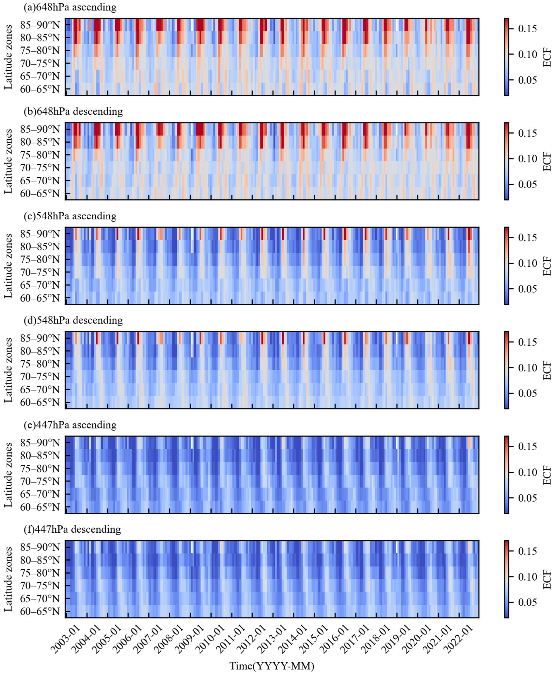
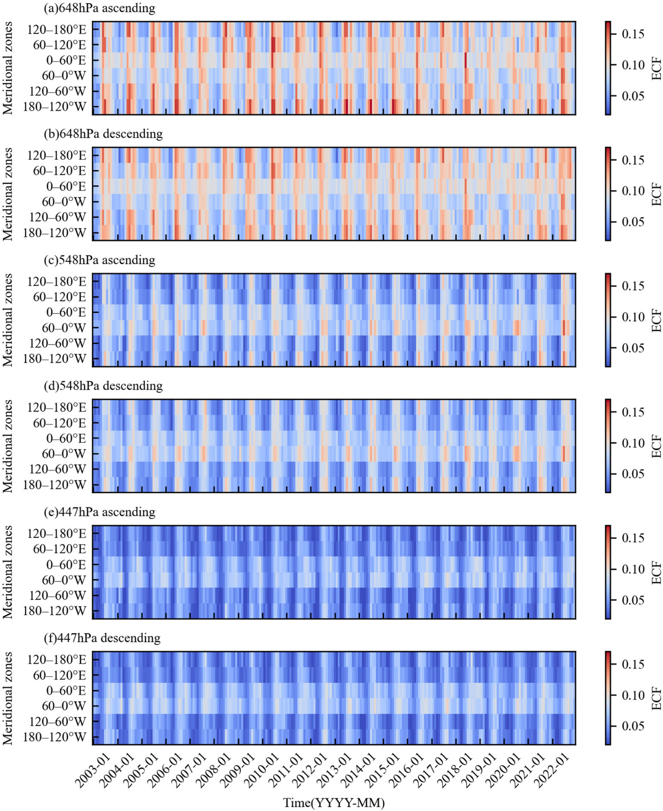
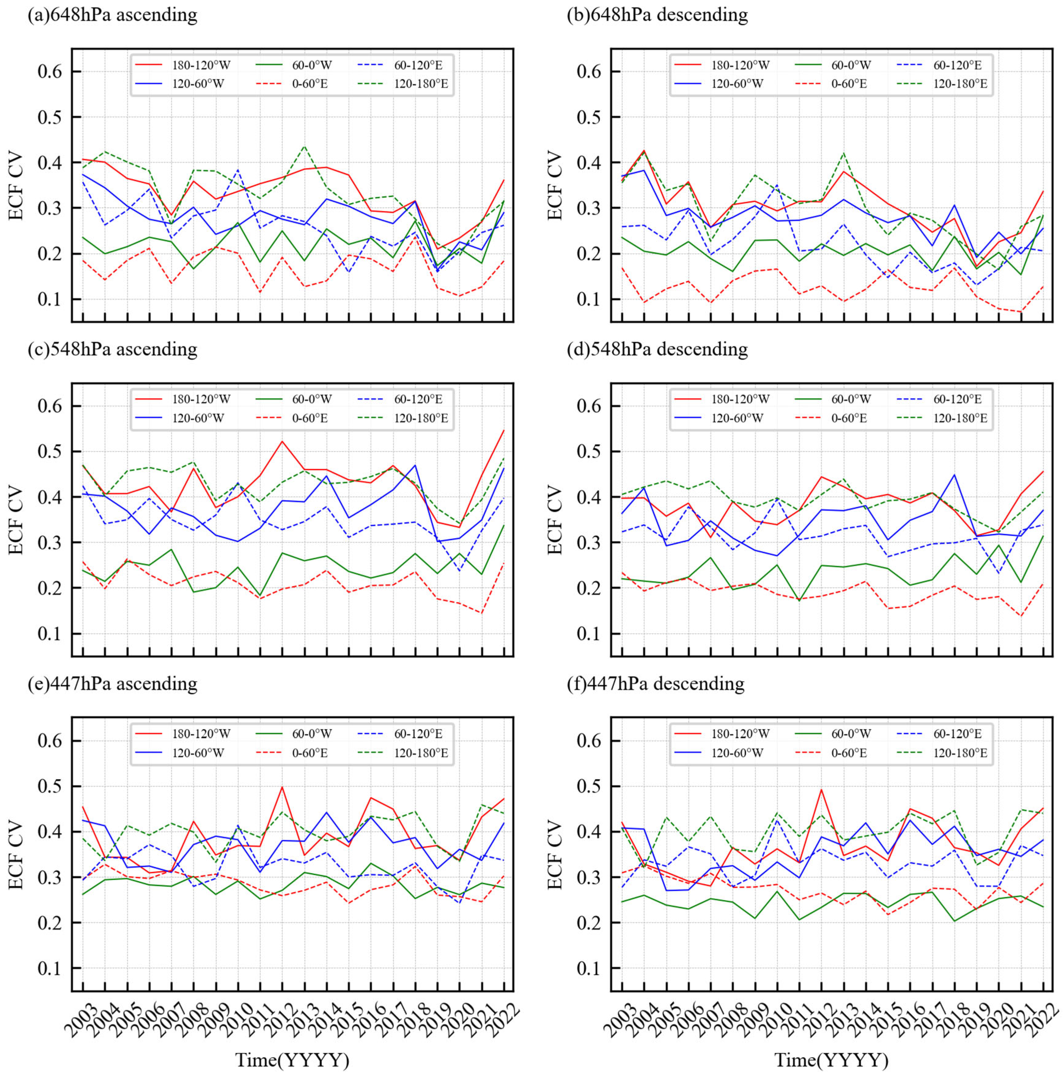
3.1. Seasonal Variations of AIRS Mid-Level ECF
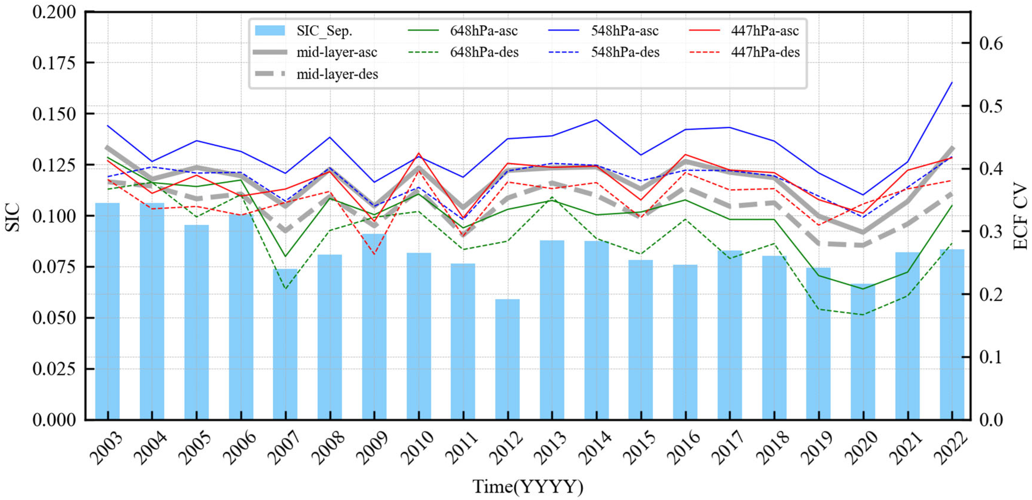
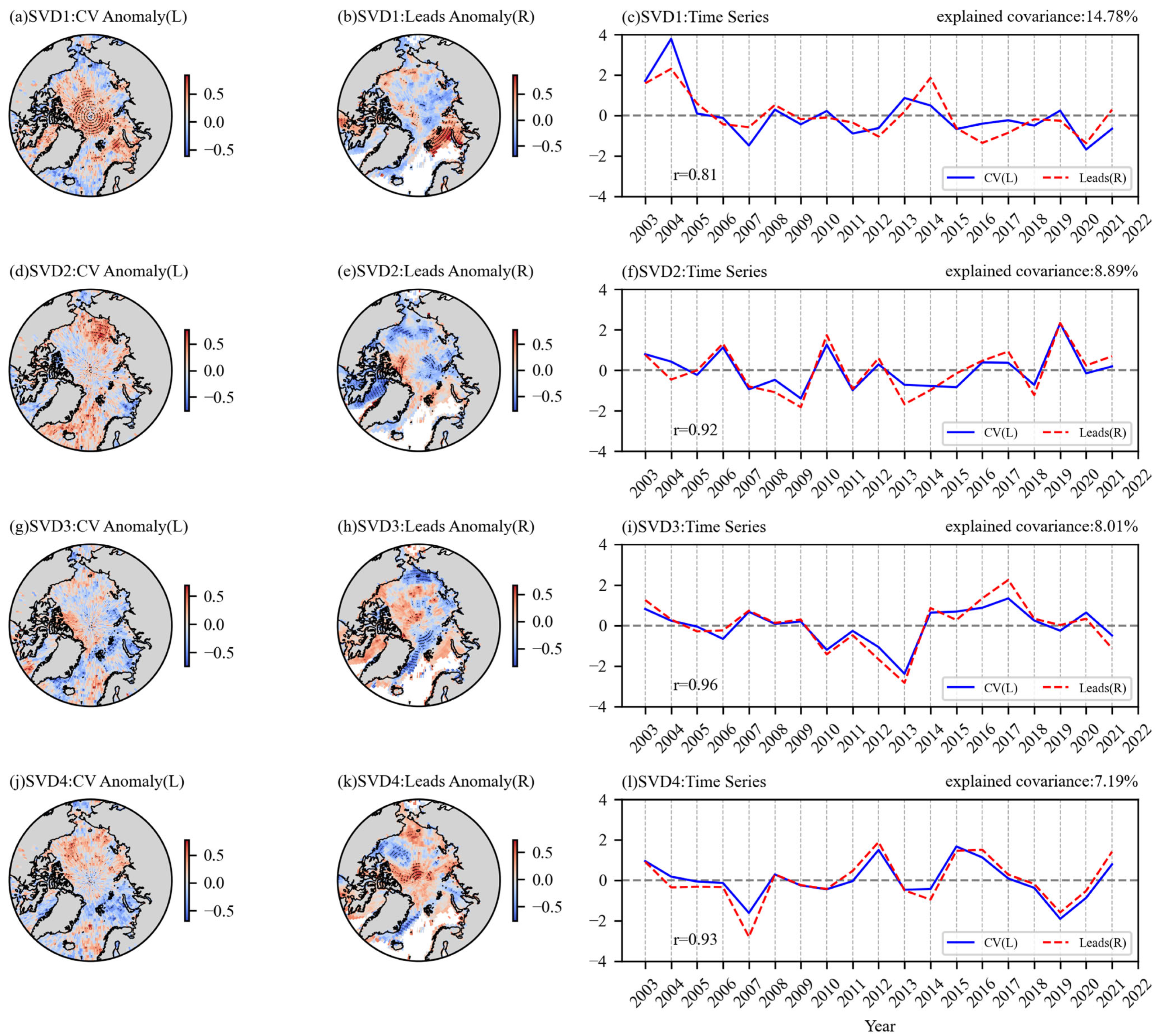
3.2. Relationships between AIRS Mid-Level ECF and the Arctic Sea Ice
4. Discussion
- (1)
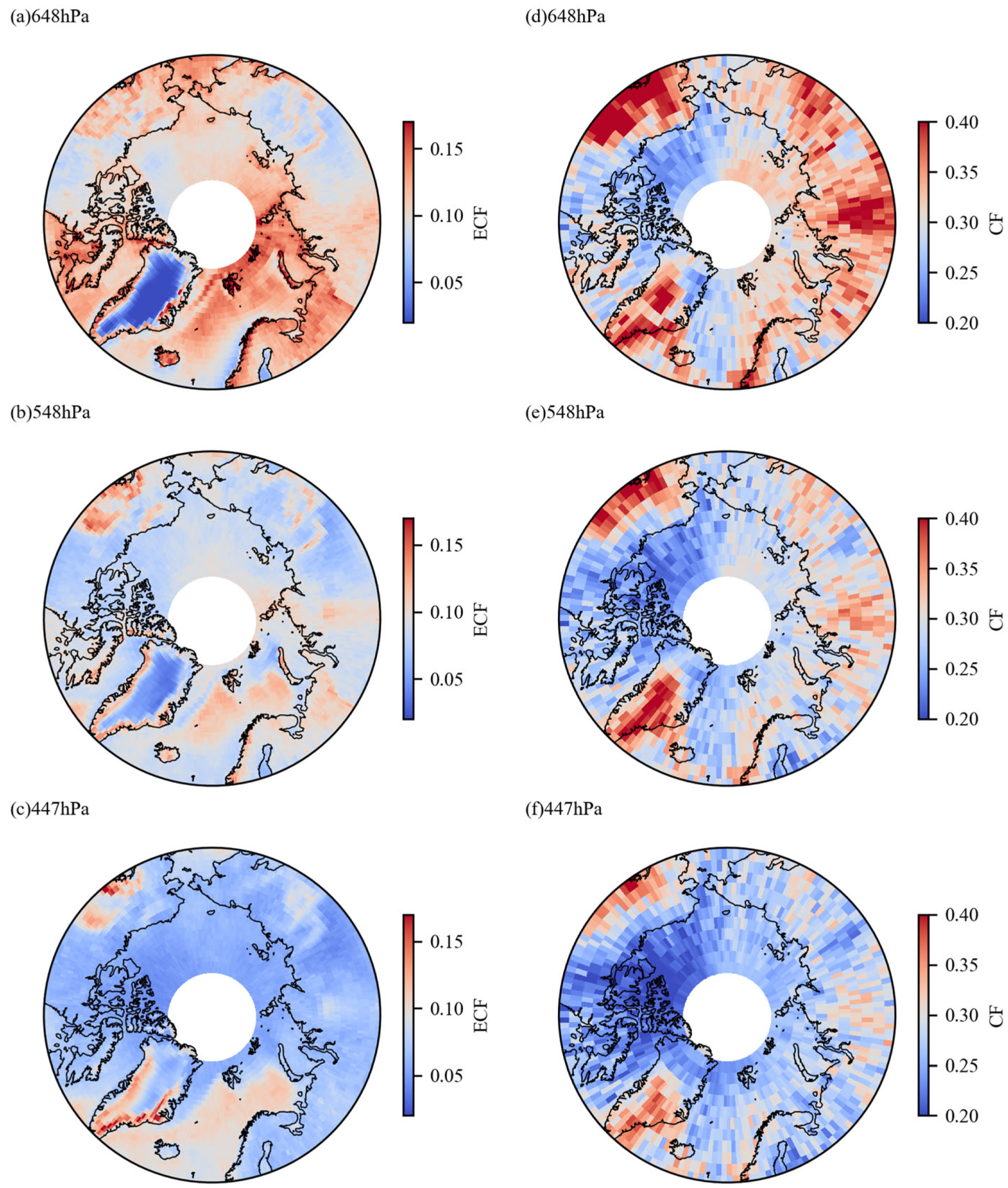
- The AIRS L3 standard product contains gridded retrieved parameters on the standard pressure levels roughly matching instrument vertical resolution. As we mentioned in Section 2.1, the effective cloud fractions are provided at 12 pressure layers. Clouds of only three pressure layers (648, 548, and 447 hPa) could be used to demonstrate the variations in mid-level clouds in the Arctic. Due to the numbers of discrete pressure levels, it may have certain limitations in capturing the fine-structured features of the mid-level clouds. However, through the preliminary comparisons with CC vertical clouds, which have a vertical resolution of 480 m, it reveals that AIRS vertical clouds above 2 km could basically represent the vertical distributions of clouds in the Arctic. Moreover, the spatial distribution of mid-level clouds is highly consistent with CC except for the controversial Greenland. Therefore, it suggests that AIRS vertical cloud fraction has the ability to represent the seasonal and annual cycle, and is useful in climatological anomaly studies, especially for the Arctic region, where persistent large-scale vertical observations for clouds are very rare.
- (2)
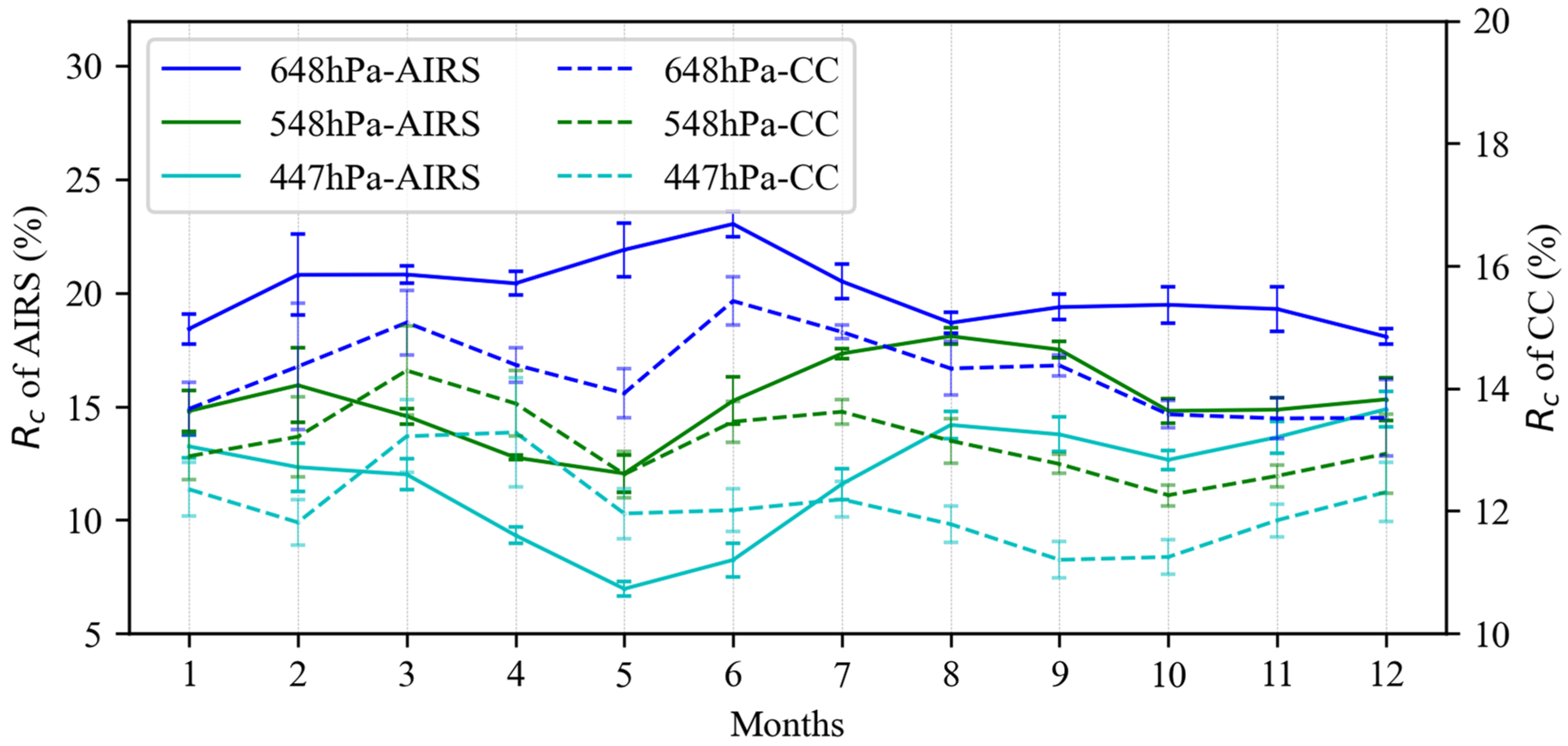
- The cloud fraction used here is the ECF, a combination of cloud fraction and cloud emissivity, which is retrieved under the assumption that the cloud emissivity is spectrally flat [20]. It is retrieved by comparing observed AIRS radiance and calculated ones of channels sensitive to cloud amount and height, after cloud-clearing steps [50]. ECF has some differences to what is commonly referred to as cloud fraction. Therefore, for comparison, ECF from AIRS and CF from CC were normalized by calculating the proportion of each layer’s ECF or CF to the total ECF or CF (accumulated over all vertical layers), in order to make the validation more reasonable. It should be noted that the original ECF is directly adopted in the follow-up analysis. On the one hand, in order to prevent the introduction of additional errors, on the other hand, preliminary validation reveals that the ECF could also characterize the variations in cloud amount, which is useful in climatological studies.
- (3)
- There are certain differences in the definition of mid-level clouds in previous studies with different regions, seasons, and observation instruments. The definition of mid-level clouds used here comes from ISCCP, which considers cloud top pressure between 440 and 680 hpa. Meanwhile, American standard atmospheric profiles for Arctic summer and winter are employed here to convert between pressure and altitude. It is found that when using the summer and winter Arctic standard atmospheric profiles for pressure to height conversion of the middle layers (648, 548, and 447 hpa), the altitude is higher in summer than that in winter, with a difference of about 0.2 to 0.4 km. For comparisons with CC, the average summer and winter Arctic profile is applied here to perform the pressure and height conversion, which is relatively more accurate for representing the multi-year average state. In addition, it should be noted that for the clouds at 648 hpa of AIRS, their upper and lower boundary layers are 600 and 700 hpa, respectively. This indicates that 648 hpa actually contains parts of the low-level clouds, which may introduce certain analysis errors.
- (4)
- When analyzing the correlations between seasonal variations in mid-level clouds and sea ice, the results obtained only based on the satellite observations used in this study may have some limitations. It has been demonstrated that changes in Arctic sea ice are influenced by various factors involved in complex mechanisms. Clouds impact the formations and variations of sea ice through their influence on radiation and related feedback mechanisms. Apart from clouds, atmospheric and oceanic circulation, as well as the coupling interactions, are also crucial factors in evaluating sea ice changes. To accurately assess the connection between clouds and sea ice, it is essential to isolate clouds from other influencing elements. This can be achieved by introducing more comprehensive and precise observational data and employing a more rational and advanced approach. In this study, our primary focus is on examining the long-term seasonal changes in Arctic mid-level clouds and conducting an initial analysis of the potential linkage between these changes and sea ice. Further in-depth research is warranted to investigate the mechanisms.
5. Conclusions
Author Contributions
Funding
Data Availability Statement
Acknowledgments
Conflicts of Interest
References
- Spänkuch, D.; Hellmuth, O.; Görsdorf, U. What Is a Cloud? Toward a More Precise Definition. Bull. Am. Meteorol. Soc. 2022, 103, E1894–E1929. [Google Scholar] [CrossRef]
- Stubenrauch, C.J.; Chédin, A.; Rädel, G.; Scott, N.A.; Serrar, S. Cloud Properties and Their Seasonal and Diurnal Variability from TOVS Path-B. J. Clim. 2006, 19, 5531–5553. [Google Scholar] [CrossRef]
- Sutphin, A.B. Characteristics of Tropical Midlevel Clouds Using A-Train Measurements. Master’s Thesis, Texas A&M University, Bizzell, TX, USA, 2013. [Google Scholar]
- Jin, H. Satellite Remote Sensing of Mid-Level Clouds. Doctoral Dissertation, Texas A&M University, Bizzell, TX, USA, 2012. [Google Scholar]
- Rossow, W.B.; Zhang, Y. Evaluation of a Statistical Model of Cloud Vertical Structure Using Combined CloudSat and CALIPSO Cloud Layer Profiles. J. Clim. 2010, 23, 6641–6653. [Google Scholar] [CrossRef]
- Zhang, D.; Wang, Z.; Liu, D. A global view of midlevel liquid-layer topped stratiform cloud distribution and phase partition from CALIPSO and CloudSat measurements. J. Geophys. Res. 2010, 115, D00H13. [Google Scholar] [CrossRef]
- Hobbs, P.V.; Rangno, A.L. Microstructures of low and middle-level clouds over the Beaufort Sea. Q. J. R. Meteorol. Soc. 1998, 124, 2035–2071. [Google Scholar] [CrossRef]
- Intrieri, J.M.; Shupe, M.D.; Uttal, T.; McCarty, B.J. An annual cycle of Arctic cloud characteristics observed by radar and lidar at SHEBA. J. Geophys. Res. Ocean. 2002, 107, SHE 5-1–SHE 5-15. [Google Scholar] [CrossRef]
- Shupe, M.D.; Walden, V.P.; Eloranta, E.; Uttal, T.; Campbell, J.R.; Starkweather, S.M.; Shiobara, M. Clouds at Arctic Atmospheric Observatories. Part I: Occurrence and Macrophysical Properties. J. Appl. Meteorol. Climatol. 2011, 50, 626–644. [Google Scholar] [CrossRef]
- Shupe, M.D. Clouds at Arctic Atmospheric Observatories. Part II: Thermodynamic Phase Characteristics. J. Appl. Meteorol. Climatol. 2011, 50, 645–661. [Google Scholar] [CrossRef]
- Yan, Y.; Liu, X.; Liu, Y.; Lu, J. Comparison of mixed-phase clouds over the Arctic and the Tibetan Plateau: Seasonality and vertical structure of cloud radiative effects. Clim. Dyn. 2020, 54, 4811–4822. [Google Scholar] [CrossRef]
- Achtert, P.; O’Connor, E.J.; Brooks, I.M.; Sotiropoulou, G.; Shupe, M.D.; Pospichal, B.; Brooks, B.J.; Tjernström, M. Properties of Arctic liquid and mixed-phase clouds from shipborne Cloudnet observations during ACSE 2014. Atmos. Chem. Phys. 2020, 20, 14983–15002. [Google Scholar] [CrossRef]
- Riihimaki, L.D.; McFarlane, S.A.; Comstock, J.M. Climatology and Formation of Tropical Midlevel Clouds at the Darwin ARM Site. J. Clim. 2012, 25, 6835–6850. [Google Scholar] [CrossRef]
- Adebiyi, A.A.; Zuidema, P.; Chang, I.; Burton, S.P.; Cairns, B. Mid-level clouds are frequent above the southeast Atlantic stratocumulus clouds. Atmos. Chem. Phys. 2020, 20, 11025–11043. [Google Scholar] [CrossRef]
- Fleishauer, R.P.; Larson, V.E.; Vonder Haar, T.H. Observed Microphysical Structure of Midlevel, Mixed-Phase Clouds. J. Atmos. Sci. 2002, 59, 1779–1804. [Google Scholar] [CrossRef]
- Bourgeois, Q.; Ekman, A.M.L.; Igel, M.R.; Krejci, R. Ubiquity and impact of thin mid-level clouds in the tropics. Nat. Commun. 2016, 7, 12432. [Google Scholar] [CrossRef] [PubMed]
- Mantsis, D.F.; Sherwood, S.; Dixit, V.; Morrison, H.; Thompson, G. Mid-level clouds over the Sahara in a convection-permitting regional model. Clim. Dyn. 2020, 54, 3425–3439. [Google Scholar] [CrossRef]
- Bourgeois, E.; Bouniol, D.; Couvreux, F.; Guichard, F.; Marsham, J.H.; Garcia-Carreras, L.; Birch, C.E.; Parker, D.J. Characteristics of mid-level clouds over West Africa. Q. J. R. Meteorol. Soc. 2018, 144, 426–442. [Google Scholar] [CrossRef]
- Lacour, A.; Chepfer, H.; Shupe, M.D.; Miller, N.B.; Noel, V.; Kay, J.; Turner, D.D.; Guzman, R. Greenland Clouds Observed in CALIPSO-GOCCP: Comparison with Ground-Based Summit Observations. J. Clim. 2017, 30, 6065–6083. [Google Scholar] [CrossRef]
- Kahn, B.H.; Irion, F.W.; Dang, V.T.; Manning, E.M.; Nasiri, S.L.; Naud, C.M.; Blaisdell, J.M.; Schreier, M.M.; Yue, Q.; Bowman, K.W.; et al. The Atmospheric Infrared Sounder version 6 cloud products. Atmos. Chem. Phys. 2014, 14, 399–426. [Google Scholar] [CrossRef]
- Susskind, J.; Barnet, C.D.; Blaisdell, J.M. Retrieval of atmospheric and surface parameters from AIRS/AMSU/HSB data in the presence of clouds. IEEE Trans. Geosci. Remote Sens. 2003, 41, 390–409. [Google Scholar] [CrossRef]
- Le Marshall, J.; Jung, J.; Derber, J.; Chahine, M.; Treadon, R.; Lord, S.J.; Goldberg, M.; Wolf, W.; Liu, H.C.; Joiner, J.; et al. Improving Global Analysis and Forecasting with AIRS. Bull. Am. Meteorol. Soc. 2006, 87, 891–895. [Google Scholar] [CrossRef]
- Smith, N.; Barnet, C.D. CLIMCAPS observing capability for temperature, moisture, and trace gases from AIRS/AMSU and CrIS/ATMS. Atmos. Meas. Tech. 2020, 13, 4437–4459. [Google Scholar] [CrossRef]
- Devasthale, A.; Sedlar, J.; Kahn, B.H.; Tjernström, M.; Fetzer, E.J.; Tian, B.; Teixeira, J.; Pagano, T.S. A Decade of Spaceborne Observations of the Arctic Atmosphere: Novel Insights from NASA’s AIRS Instrument. Bull. Am. Meteorol. Soc. 2016, 97, 2163–2176. [Google Scholar] [CrossRef]
- Chang, L.; Feng, G.; Zhang, Y.; He, X. Effect of Cloud Fraction on Arctic Low-Level Temperature Inversions in AIRS Observations Over Both Land and Ocean. IEEE Trans. Geosci. Remote Sens. 2018, 56, 2025–2032. [Google Scholar] [CrossRef]
- Chang, L.; Chen, F.; Gao, G.; Zhang, Y. Effects of Water Vapor and Cloud Fraction in AIRS Retrievals on Arctic Sea Ice Variability. IEEE Trans. Geosci. Remote Sens. 2022, 60, 1–12. [Google Scholar] [CrossRef]
- Tian, B.; Manning, E.; Roman, J.; Thrastarson, H.; Fetzer, E.; Monarrez, R. AIRS Version 7 Level 3 Product User Guide. Available online: https://docserver.gesdisc.eosdis.nasa.gov/public/project/AIRS/V7_L3_Product_User_Guide.pdf (accessed on 18 December 2023).
- Susskind, J.; Blaisdell, J.; Iredell, L.; Lee, J.; Milstein, A.; Barnet, C.; Fishbein, E.; Manning, E.; Strow, L.; Teixeira, J. Algorithm Theoretical Basis Document-Airs-Team Retrieval for Core Products and Geophysical Parameters: Versions 6 and 7 Level 2. Available online: https://docserver.gesdisc.eosdis.nasa.gov/public/project/AIRS/L2_ATBD.pdf (accessed on 18 December 2023).
- Manning, E.; Kahn, B.; Fetzer, E.J.; Yue, Q.; Wong, S.; Kalmus, P.; Payne, V.; Wang, T.; Olsen, E.T.; Wilson, R.C.; et al. AIRS/AMSU/HSB Version 7 Level 2 Product User Guide. Available online: https://docserver.gesdisc.eosdis.nasa.gov/public/project/AIRS/V7_L2_Product_User_Guide.pdf (accessed on 18 December 2023).
- Blaisdell, J.M.; Farahmand, A.; Fetzer, E.J.; Fishbein, E.; Griffin, E.; Iredell, L.; Irion, F.W.; Kahn, B.H.; Kalmus, P.; Manning, E.; et al. AIRS Version 7 Level 2 Performance Test and Validation Report. Available online: https://docserver.gesdisc.eosdis.nasa.gov/public/project/AIRS/V7_L2_Performance_Test_and_Validation_report.pdf (accessed on 18 December 2023).
- Kay, J.E.; L’Ecuyer, T.; Gettelman, A.; Stephens, G.; O’Dell, C. The contribution of cloud and radiation anomalies to the 2007 Arctic sea ice extent minimum. Geophys. Res. Lett. 2008, 35, L08503. [Google Scholar] [CrossRef]
- Kay, J.E.; Gettelman, A. Cloud influence on and response to seasonal Arctic sea ice loss. J. Geophys. Res. Atmos. 2009, 114, D18204. [Google Scholar] [CrossRef]
- Mace, G.G.; Zhang, Q.; Vaughan, M.; Marchand, R.; Stephens, G.; Trepte, C.; Winker, D. A description of hydrometeor layer occurrence statistics derived from the first year of merged Cloudsat and CALIPSO data. J. Geophys. Res. Atmos. 2009, 114, D00A26. [Google Scholar] [CrossRef]
- Mace, G.G.; Benson, S.; Kato, S. Cloud radiative forcing at the Atmospheric Radiation Measurement Program Climate Research Facility: 2. Vertical redistribution of radiant energy by clouds. J. Geophys. Res. Atmos. 2006, 111, D11S91. [Google Scholar] [CrossRef]
- Rossow, W.B.; Schiffer, R.A. Advances in Understanding Clouds from ISCCP. Bull. Am. Meteorol. Soc. 1999, 80, 2261–2288. [Google Scholar] [CrossRef]
- Weare, B.C. Insights into the importance of cloud vertical structure in climate. Geophys. Res. Lett. 2000, 27, 907–910. [Google Scholar] [CrossRef]
- Liu, X.; He, T.; Sun, L.; Xiao, X.; Liang, S.; Li, S. Analysis of Daytime Cloud Fraction Spatiotemporal Variation over the Arctic from 2000 to 2019 from Multiple Satellite Products. J. Clim. 2022, 35, 7595–7623. [Google Scholar] [CrossRef]
- Meier, W.N.; Fetterer, F.; Savoie, M.; Mallory, S.; Duerr, R.; Stroeve, J. NOAA/NSIDC Climate Data Record of Passive Microwave Sea Ice Concentration; Version 3 [Data Set]; NSIDC: Boulder, CO, USA, 2017. [Google Scholar] [CrossRef]
- Windnagel, A. NOAA/NSIDC Climate Data Record of Passive Microwave Sea Ice Concentration, Version 3 User Guide. Available online: https://nsidc.org/sites/nsidc.org/files/G02202-V001-UserGuide.pdf (accessed on 18 December 2023).
- Reiser, F.; Willmes, S.; Heinemann, G. A New Algorithm for Daily Sea Ice Lead Identification in the Arctic and Antarctic Winter from Thermal-Infrared Satellite Imagery. Remote Sens. 2020, 12, 1957. [Google Scholar] [CrossRef]
- Reiser, F.; Willmes, S.; Heinemann, G. Daily Sea Ice Lead Data for Arctic and Antarctic. 2020. Available online: https://doi.org/10.1594/PANGAEA.917588 (accessed on 27 December 2023).
- Parkinson, C.L.; Comiso, J.C. On the 2012 record low Arctic sea ice cover: Combined impact of preconditioning and an August storm. Geophys. Res. Lett. 2013, 40, 1356–1361. [Google Scholar] [CrossRef]
- Zhang, J.; Lindsay, R.; Schweiger, A.; Steele, M. The impact of an intense summer cyclone on 2012 Arctic sea ice retreat. Geophys. Res. Lett. 2013, 40, 720–726. [Google Scholar] [CrossRef]
- Jeong, H.; Park, H.-S.; Stuecker, M.F.; Yeh, S.-W. Record Low Arctic Sea Ice Extent in 2012 Linked to Two-Year La Niña-Driven Sea Surface Temperature Pattern. Geophys. Res. Lett. 2022, 49, e2022GL098385. [Google Scholar] [CrossRef]
- Zhu, J.; Yu, Y.; Guan, Z.; Wang, X. Dominant Coupling Mode of SST in Maritime Continental Region and East Asian Summer Monsoon Circulation. J. Geophys. Res. Atmos. 2022, 127, e2022JD036739. [Google Scholar] [CrossRef]
- Ma, J.; Xie, S.-P.; Xu, H. Contributions of the North Pacific Meridional Mode to Ensemble Spread of ENSO Prediction. J. Clim. 2017, 30, 9167–9181. [Google Scholar] [CrossRef]
- Chatterjee, S.; Raj, R.P.; Bertino, L.; Mernild, S.H.; Subeesh, M.P.; Murukesh, N.; Ravichandran, M. Combined influence of oceanic and atmospheric circulations on Greenland sea ice concentration. Cryosphere 2021, 15, 1307–1319. [Google Scholar] [CrossRef]
- Li, X.; Krueger, S.K.; Strong, C.; Mace, G.G. Relationship Between Wintertime Leads and Low Clouds in the Pan-Arctic. J. Geophys. Res. Atmos. 2020, 125, e2020JD032595. [Google Scholar] [CrossRef]
- Pagano, T.S.; Payne, V.H. The Atmospheric Infrared Sounder. In Handbook of Air Quality and Climate Change; Akimoto, H., Tanimoto, H., Eds.; Springer: Singapore, 2020; pp. 1–13. [Google Scholar]
- Kahn, B.H.; Eldering, A.; Braverman, A.J.; Fetzer, E.J.; Jiang, J.H.; Fishbein, E.; Wu, D.L. Toward the characterization of upper tropospheric clouds using Atmospheric Infrared Sounder and Microwave Limb Sounder observations. J. Geophys. Res. Atmos. 2007, 112, D05202. [Google Scholar] [CrossRef]


| Layers (hPa) | Percent of ECF (%) | Layers (hPa) | Percent of ECF (%) | ||
|---|---|---|---|---|---|
| Ascending | Descending | Ascending | Descending | ||
| 1018 | 4.9822 | 5.8111 | 346 | 9.1497 | 9.6849 |
| 887 | 8.5849 | 8.0757 | 274 | 2.8735 | 3.1472 |
| 771 | 25.7638 | 23.1594 | 224 | 1.0029 | 1.1303 |
| 648 | 21.2827 | 21.3865 | 173 | 0.0838 | 0.1047 |
| 548 | 14.9392 | 15.5300 | 122 | 0.0003 | 0.0003 |
| 447 | 11.3360 | 11.9693 | 32 | 0.0003 | 0.0002 |
Disclaimer/Publisher’s Note: The statements, opinions and data contained in all publications are solely those of the individual author(s) and contributor(s) and not of MDPI and/or the editor(s). MDPI and/or the editor(s) disclaim responsibility for any injury to people or property resulting from any ideas, methods, instructions or products referred to in the content. |
© 2024 by the authors. Licensee MDPI, Basel, Switzerland. This article is an open access article distributed under the terms and conditions of the Creative Commons Attribution (CC BY) license (https://creativecommons.org/licenses/by/4.0/).
Share and Cite
Wang, X.; Liu, J.; Liu, H. Seasonal Variability of Arctic Mid-Level Clouds and the Relationships with Sea Ice from 2003 to 2022: A Satellite Perspective. Remote Sens. 2024, 16, 202. https://doi.org/10.3390/rs16010202
Wang X, Liu J, Liu H. Seasonal Variability of Arctic Mid-Level Clouds and the Relationships with Sea Ice from 2003 to 2022: A Satellite Perspective. Remote Sensing. 2024; 16(1):202. https://doi.org/10.3390/rs16010202
Chicago/Turabian StyleWang, Xi, Jian Liu, and Hui Liu. 2024. "Seasonal Variability of Arctic Mid-Level Clouds and the Relationships with Sea Ice from 2003 to 2022: A Satellite Perspective" Remote Sensing 16, no. 1: 202. https://doi.org/10.3390/rs16010202
APA StyleWang, X., Liu, J., & Liu, H. (2024). Seasonal Variability of Arctic Mid-Level Clouds and the Relationships with Sea Ice from 2003 to 2022: A Satellite Perspective. Remote Sensing, 16(1), 202. https://doi.org/10.3390/rs16010202