Abstract
Transpiration (T) represents plant water use, while sun-induced chlorophyll fluorescence (SIF) emitted during photosynthesis, relates well to gross primary production. SIF can be influenced by vegetation structure, while uncertainties remain on how this might impact the relationship between SIF and T, especially for open and sparse woodlands. In this study, a method was developed to map T in riverine floodplain open woodland environments using satellite data coupled with a radiative transfer model (RTM). Specifically, we used FluorFLiES, a three-dimensional SIF RTM, to simulate the full spectrum of SIF for three open woodland sites with varying fractional vegetation cover. Five specific SIF bands were selected to quantify their correlation with field measured T derived from sap flow sensors. The coefficient of determination of the simulated far-red SIF and field measured T at a monthly scale was 0.93. However, when comparing red SIF from leaf scale to canopy scale to predict T, performance declined by 24%. In addition, varying soil reflectance and understory leaf area index had little effect on the correlation between SIF and T. The method developed can be applied regionally to predict tree water use using remotely sensed SIF datasets in areas of low data availability or accessibility.
1. Introduction
The global water cycle represents the water exchange between the Earth and the atmosphere, which impacts water supply to vegetation and all living entities [1,2,3]. In recent years, human intervention has increasingly impacted the water cycle through activities including dam construction, river flow management [4,5], and, more indirectly, from climate change-driven floods and droughts [6,7]. The impacts of these human disturbances require close monitoring to enable the planning of adaptions and mitigations for future hydrological and climatological perturbations. Routine evapotranspiration (ET) monitoring is required to assess human impacts by describing the sum of water transfer from the ground through soil evaporation and plant transpiration (T) via leaf stomata [8,9,10]. In general, T or plant water use accounts for more than 65% of the total terrestrial ET for mature forested ecosystems [11] and exhibits a strong relationship with photosynthetic activity, where leaf stomatal conductance controls the rate of T and, hence, the uptake of water and CO2 during photosynthesis [12]. Accurate estimation of T can, therefore, improve our understanding of the coupling of the global water and carbon cycle [13].
Monitoring T from space, however, remains highly challenging. Previous studies have incorporated empirical equations to constrain T based on remotely sensed vegetation indices and land surface models [14,15]. Researchers also rely on a variety of methods to estimate T, including the widely used Penman-Monteith (P-M) and Priestley-Taylor (P-T) equations [16,17], where T can be estimated using meteorological data, including measurements of incoming radiation, air temperature, wind speed, and relative humidity. However, these models are insufficient in modelling T using remote sensing data in sparse woodlands due to an assumption of surface uniformity. More direct T estimates are derived from eddy covariance flux tower data by partitioning ET into evaporation and T [18]. Alternatively, sap flow sensors collecting sap flow velocity data from individual trees can be scaled to the ‘plot’ level once correction and scaling factors are incorporated [19,20,21]. However, these techniques are limited in their spatial representativeness and coverage, and uncertainties remain in upscaling T from plot-scale to watershed and global scales using remote sensing techniques. Reducing these uncertainties would enable a more accurate determination of global water cycles [22].
Sun-induced chlorophyll fluorescence (SIF) provides a promising proxy to monitor vegetation photosynthetic activity, especially for water-stressed vegetation [23,24]. Chlorophyll fluorescence refers to the emission of light from chlorophyll during photosynthesis and occurs in the light spectrum between 640 to 850 nanometres (nm). Advanced hyperspectral sensors that operate on flux towers, drones, and from space, provide a novel means to retrieve SIF and to monitor carbon uptake across spatiotemporal scales [25,26,27].
There are two typical SIF retrieval bands in the SIF spectrum, the first being in the red region (680 nm), which largely contains photosynthesis system II (PSII) information, and the other in the far-red region (740 nm), which provides information about both photosynthesis system I (PSI) and PSII [28,29]. Photosynthesis systems I and PSII coordinate leaf pigments, including chlorophyll content and carotenoids, to harvest light energy that drives photosynthesis [30,31]. Additionally, other SIF bands provide responses to environmental stress and reflect plant physiological conditions [32]. It is expected that multiple SIF bands can be employed to understand vegetation responses to varying climate and water availability. However, due to sensor and retrieval algorithm limitations, remote SIF retrievals, including satellites (GOME-2, OCO-2 and TROPOMI), only provide SIF retrievals in the red band and far-red region.
It has been determined that far-red SIF correlates well with gross primary production (GPP) over regions with dense canopy cover [33,34,35]. However, coarse spatial resolution (>1 km) of satellite SIF products and limited band retrievals mean knowledge gaps exist in understanding the relationship between SIF bands and plant physiological functioning across ecosystems. Earlier investigations have established strong correlations between far-red SIF and T in dense temperate forests [36], while environmental factors such as shortwave radiation, temperature, and relative humidity impacted the SIF–T relationship for a mature, well-watered forest [37]. Maes [38] demonstrated that using SIF to predict T was more effective than using remotely sensed vegetation indices and that seasonal variations of SIF were similar to T for various plant functional types. Additionally, the SIF–T relationship has been used for evaluating vegetation water stress. For example, coupling vapour pressure deficit with SIF was able to improve T estimation [39], assessing the sensitivity of SIF-based T estimating considering soil water limitations [40], applying SIF to deliver global transpiration estimates [15], and partitioning T from ET based on a SIF-driven model [41]. However, these studies focused on SIF emissions in the far-red region (740 nm and 760 nm), and hence, the correlation between T and other specific SIF bands remains unknown.
Reviewing prior studies of SIF–T relationship, research gaps are coarse spatial resolutions of SIF observations leading to the unavailability of fine-scale SIF datasets in Australia, unknown relationships between various SIF bands and T, a lack of comprehensive study on sparse forest scenes, and uncertainty of vegetation structure impacts on SIF–T relationships. Low temporal and spatial resolutions of SIF products mean these products are limited in their ability to validate predictions of T for open woodlands, as low canopy cover and soil background add noise to SIF signals [42,43]. To overcome these issues, radiative transfer models (RTMs) are an effective tool to assess these relationships for complex scenes with defined spatial and temporal resolution. By accurately modelling complex vegetation structure, leaf physiological properties, and simulating multiple bands in SIF emission spectral regions, RTMs could be helpful for studying the relationship between SIF and T for open woodlands across various scales [42,44,45,46]. A study by Lu [36] incorporated field-obtained far-red SIF with a one-dimensional (1-D) RTM to reconstruct the full SIF spectrum and analyse the relationship between specific SIF bands and P-M/P-T derived T, using eddy covariance data. However, T was not directly measured, and there is a mismatch between the scale of measurement for in situ SIF [47] and eddy covariance data, which presents gas exchange for up to a radius of 1 km [48]. Although near-infrared (NIR) SIF emissions appear better for explaining variations in T rather than the red region for American Beech and red oak [36], this relationship was uncertain for other tree species. Lastly, while RTMs have been used to infer the full SIF shape and are beneficial to investigate the predictive power of SIF across the SIF spectrum, a 1-D RTM was unable to accurately simulate SIF for complex and multi-layer vegetation structures, especially for sparse woodlands, as 1-D RTMs are more suitable for use with uniform canopy layers that possess less vertical structure variations [42]. A further knowledge gap is apparent in relation to the influence of vegetation structure characteristics such as leaf area index (LAI) and fractional vegetation cover (FVC) on SIF [42,45]. As 1-D RTMs contain limited vegetation structure parameters, they are unable to precisely describe vertical and horizontal vegetation structures; hence, much uncertainty exists around using SIF to predict T across heterogenous areas, particularly open woodland areas.
In Australia’s Murray–Darling Basin (MDB), a river basin of ~1,000,000 km2, accurate but resource-intensive methods are employed to accurately monitor woody vegetation T and ET to enhance our understanding of tree water requirements [19,49]. While these in situ studies are critical for providing empirical data presented in and across many other studies [19,49,50], broadscale and long-term in situ measurements are not feasible. Currently, in situ ET measurements in the MDB are scaled regionally using remote sensing [50,51]. However, substituting in situ T with SIF-derived data is likely to allow for future efficiencies while maintaining data rigour and improving our spatial and temporal understanding of both water requirements and tree response to human activities and climate change across a geographically broad river basin.
Hence, the overarching aim of this study is to study SIF performance from diverse bands to explain seasonal variations of in situ measured T for open woodlands. A method was developed for retrieving vegetation functional and structural traits, and a three-dimensional (3-D) RTM was applied to simulate SIF for three open woodland sites with varying FVC in the MDB. Specifically, the objectives were to: (1) evaluate the correlation between in situ T collected using sap flow sensors and simulated SIF at multiple bands across hourly to monthly temporal scales; (2) quantify the correlation between in situ T and SIF simulations from leaf level and canopy level; and (3) conduct sensitivity simulations to quantify the influence of vegetation structure on the SIF–T relationship. The study comprises three open woodland environments characteristic of the MDB, across two native tree species, with a range of foliage cover (FVC 0.1–0.5). These sites encapsulate trees with good access to fresh water sources and hence, higher canopy density, through to the converse in shallow saline groundwater environments, to assess the SIF–T relationship in low and high canopy circumstances. It is anticipated this study will provide novel and vital timeseries data to further our understanding of open woodland tree responses to disturbances such as climate and human-induced drought. More importantly, it demonstrates a new method to scale T more broadly and efficiently in open woodlands, applicable both in Australia and worldwide.
2. Materials and Methods
2.1. Study Area
The Murray–Darling Basin is located across five states and territories in southeastern Australia, covering ~14% of Australia’s land area [52]. Irrigation is the lifeblood for what is known as Australia’s food bowl, but the region is semi-arid and experiences frequent and often long-term droughts [53]. The annual mean temperature in the study region is ~18 °C with mean annual precipitation ~270 mm. However, during the Austral summer (December to February), maximum temperatures predominantly exceed 32 °C and peak for several days, >44 °C over summer.
Woody vegetation in the southern MDB is predominantly composed of two key tree species: Eucalyptus camaldulensis (River Red Gum) and E. largiflorens (Black Box). Each species has specific water requirements and salinity tolerances [54], with E. camaldulensis being more flood-tolerant but less salt-tolerant than E. largiflorens [55]. Three open woodland study sites for this research were located in the southern MDB on floodplains adjacent to the River Murray (Table 1 and Figure 1), one of three major rivers in the Basin. For the purpose of this study and depending on the FVC obtained from LiDAR data (see Section 2.3.3), the in situ sites were categorised as sparse (FVC = 0.12), moderately sparse (FVC = 0.25), and open woodland (FVC = 0.5).

Table 1.
Locations, annual mean transpiration (T), and fractional vegetation cover (FVC) for Mallee Cliffs E. largiflorens (Black Box) sparse site (MCBB_S), Mallee Cliffs Black Box moderately sparse site (MCBB_MS), and Lindsay Forest E. camaldulensis open woodland (River Red Gum).
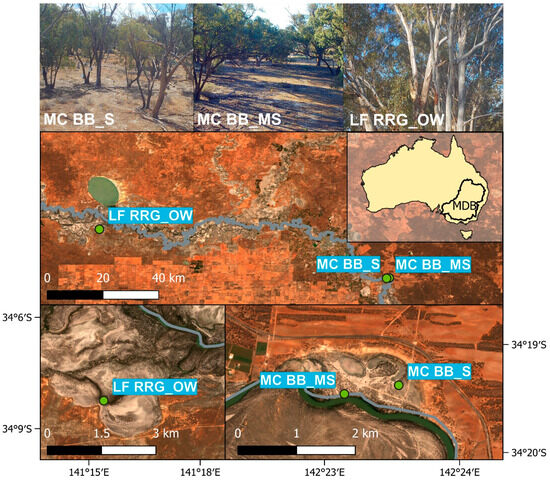
Figure 1.
Site locations of Mallee Cliffs E. largiflorens sparse site (MCBB_S), Mallee Cliffs E. largiflorens moderately sparse site (MCBB_MS), and Lindsay Forest E. camaldulensis open woodland site (LFRRG_OW) in the Murray–Darling Basin (MDB). Pictures in the first row were taken by site cameras.
The sparse and moderately sparse open woodland sites were located near Gol Gol in New South Wales and composed of Black Box trees. Tree water use monitoring at the sparse open woodland site, referred to as MCBB_S, was established in February 2019, with data collection ongoing, to monitor the effects of altered saline groundwater pumping away from the floodplain, associated with a salt interception scheme [56]. This site is located ~650 m north of the River Murray channel above highly saline shallow groundwater (46,000–55,000 EC). The moderately sparse open woodland site, MCBB_MS, is 950 m southwest of MCBB_S and 60 m north of the River Murray channel. This site is influenced by a freshened groundwater lens created via lateral bank recharge [57,58] and groundwater pumping from the salt interception scheme, providing a permanent fresh water source. The third site, LFRRG_OW, categorised as open woodland (Table 1), is located on Lindsay Island, in Victoria, ~100 m south of the River Murray and likely within the zone of lateral bank recharge [57].
2.2. Data
2.2.1. Transpiration Field Measurements
Tree transpiration was measured at each 50 × 50 m site by employing 10 SFM1 sap flow metres (ICT International, Armidale, Australia), in six trees [50]. Sample trees were determined by dividing all trees within each plot into three classes (small, medium, and large) based on the total plot stem basal area over bark. As per Benyon and Doody [59] and Doody et al. (2015), two sample trees for each class were randomly selected for sap flow measurement. Relying on the heat pulse velocity method, sap velocity and volumetric water flow in xylem tissue were determined [60]. Here, water flux was calculated by measuring the difference between heat transported between two temperature probes of the sap flow sensor. Hourly T (mm h−1) for each site was calculated as the product of hourly averaged sap flow velocity and sapwood area, estimated by using sapwood thickness of each wood core collected from each sample tree. In addition, the diameter at breast height of each tree at each site was measured annually and employed for modelling 3-D tree structure in the model. Transpiration measurements were collected from 1 June 2019, to 31 May 2021, at MCBB_S and MCBB_MS and from 16 October 2019, to 25 May 2021, at LFRRG_OW, with data recorded every 30 min.
2.2.2. LiDAR Data and Vegetation Structure
LiDAR was employed to reconstruct 3-D tree structure by using reflected laser light to densely sample objects on the earth in x, y, and z coordinates [61]. Airborne LiDAR data for each site was downloaded from a cloud-based spatial data portal ELVIS (https://elevation.fsdf.org.au/ (accessed on 22 December 2021)). Each in situ 50 × 50 m plot was cropped from the LiDAR data. The average LiDAR point density was four points per square metre, with LiDAR flown in 2013 and deemed the best available to establish overstorey canopy structure, such as tree position, crown height, crown radius, and trunk height (Section 2.3.3).
2.2.3. Satellite Remote Sensing Data
Photosynthetically active radiation (PAR), LAI, fraction of absorbed photosynthetically active radiation (FAPAR), and surface reflectance remotely sensed products were collected at the three sites to retrieve leaf structural and functional traits for model input. The epoch of June 2019 to May 2021 was selected to overlap with the in situ T data.
Himawari-8 level 3 PAR product [62]: Model input for the main driver of photosynthesis and SIF. The advanced Himawari imager provides 16 channels to capture rapidly changing weather patterns every 15 min at a 5 km spatial resolution.
Sentinel-2 LAI, FAPAR, and levels 2A surface reflectance data products: Dates with more than 10% cloud cover data were removed. Surface reflectance data varied from 10 m to 60 m and was resampled to 20 m and cropped using in situ site corner coordinates (50 ∙ 50 m). Vegetation indices (VIS2) were calculated from the surface reflectance products and included the Enhanced Vegetation Index (EVI) and Normalised Difference Vegetation Index (NDVI) as proxies of vegetation growth [63]. A Singular Spectrum Analysis (SSA) method was applied to remove noise from VIS2 and to scale it to daily timesteps [64]. Leaf area index, defined as the total one-sided leaf area per unit of ground area [65], and FAPAR representing fraction of solar radiation absorbed by leaves for photosynthesis activity [66], are two essential climate variables quantitatively related to canopy structure and function. Sentinel-2 LAI and FAPAR (referred to as LAIS2 and FAPARS2, respectively) were computed from Sentinel-2 surface reflectance data and a pre-trained neural network [67].
2.3. Method
2.3.1. Model Framework Overview
A SIF modelling framework was developed to overcome spatial, spectral, and temporal limitations of current satellite SIF products for estimating T in sparse woodland environments. In this study, diverse SIF bands (red band—685 nm, SIF valley band—699 nm, SIF water vapour band—720 nm, SIF NIR band—740 nm, SIF O2-A band—760 nm) were simulated at the hourly scale using retrieved vegetation structural and functional parameters in five steps (Figure 2). First, 3-D vegetation structure was retrieved from LiDAR data (Figure 2 and Figure S1). Sentinel-2 LAI was then partitioned into canopy and understory LAI (LAIu) to retrieve model structural input parameters (Figure 2 and Figure S2). A two-step inversion was applied to retrieve input parameters for SIF model simulations. For the first-step inversion, a relationship was developed to predict leaf area density (LAD) from LAI, which relied on a lookup table (LUT) and the LAI calculation mode of the FLiES model (Figure 2 and Figure S3a). Next, bioparameters and soil reflectance (Rsoil) were derived based on FLiES model simulations by matching Sentinel-2 vegetation indices, LAI, and FAPAR with LUT simulations (Figure 2 and Figure S3b). Combining previously retrieved vegetation structure (Figure 2 and Figure S1), leaf functional traits (Figure 2 and Figure S3a,b), incoming radiation, the 3-D model, and FluorFLiES simulated the full SIF spectrum at the hourly scale (Figure 2 and Figure S4). Finally, selected SIF bands were evaluated with in situ measured T (Figure 2 and Figure S5).
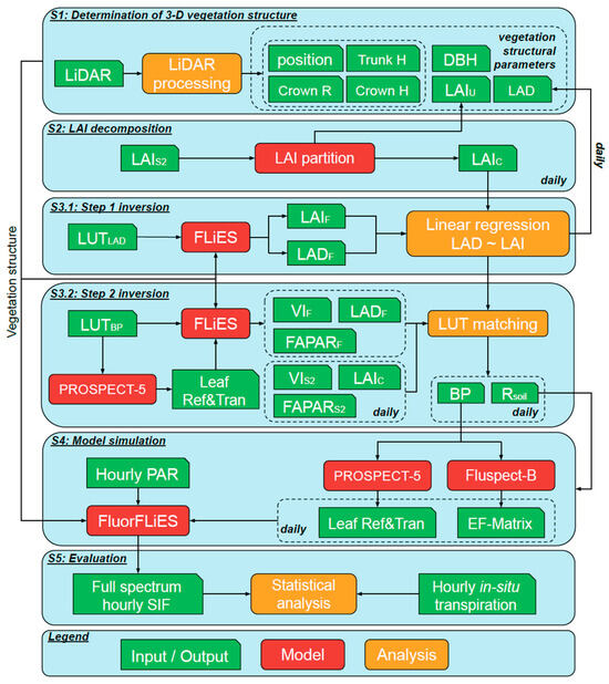
Figure 2.
Flowchart of the simulations. Step 1 (S1)—determine 3-D vegetation structure from LiDAR data. Step 2 (S2)—Sentinel-2 LAI (LAIS2) partitioned into canopy (LAIc) and understory LAI (LAIu). Step 3 (S3)—retrieve leaf area density (LAD) and six bioparameters (BP), including leaf mesophyll structure, leaf chlorophyll a + b content, total carotenoid content, senescence material, leaf dry matter content, and leaf water content, using a two-step inversion method with two lookup tables (LUTLAD and LUTBP). Step 4 (S4)—use FluorFLiES model with vegetation structure and bioparameters to simulate the full spectrum sun-induced chlorophyll fluorescence (SIF). Step 5 (S5)—statistical analysis conducted on the relationship between simulated SIF and field measured transpiration (T). Height (H); radius (R). H and R mean height and radius. Simulated LAI (LAIF), LAD (LADF), and fraction of absorbed photosynthetically active radiation (FAPARF) with the FLiES model. Leaf reflectance (ref); transmittance (tran); soil reflectance (Rsoil); excitation-fluorescence matrices (EF-matrix); photosynthetically active radiation (PAR).
2.3.2. Radiative Transfer Models
FluorFLiES, an extension of the Forest Light Environmental Simulator (FLiES) model, enables the simulation of the full spectrum of SIF from 640 to 850 nm for 3D heterogeneous vegetation [42]. Briefly, FLiES is a 3D RTM based on the Monte Carlo method [68,69] to simulate both the bidirectional reflectance factor and the distribution of absorbed PAR for complex heterogeneous forest scenes, such as the open woodland environments used in this study. The simulation landscape was divided into four layers in the model: atmosphere; canopy, understory vegetation, and soil layers (see FLiES model manual Figure 1). The FLiES photon scattering information was coupled with excitation-fluorescence matrices (EF-matrix) to simulate SIF in FluorFLiES. FluorFLiES was used in forward mode, tracing photon trajectories through the four layers to a virtual sensor located at the top of the canopy. FLiES and FluorFLiES, both open-source software, have been previously validated for several applications in forest environments [42,70,71,72]. The FluorFLiES model requires input bioparameters to generate leaf reflectance, transmittance, and the EF-matrix, which are used to generate leaf-level fluorescence emissions. FluorFLiES structural inputs (tree position, crown height, radius, trunk height, DBH, LAD, and LAIu) were parameterised from airborne LiDAR data (see Section 2.3.3), leading to an accurate spatial representation of these complex heterogeneous forest scenes.
2.3.3. Determination of 3D Vegetation Structure
Both FLiES and FluorFLiES employed the same 3D vegetation scene for each site. The simulation scene was defined as a 50 × 50 m square area for each in situ site. First, FUSION software [73] was applied to extract the digital surface model for ground elevation features and a digital terrain model for ground surface elevation. A canopy height model was calculated by finding the difference between the two models (0.5 m spatial resolution). Hence, each canopy height model pixel indicates vegetation height. Tree location (x and y coordinates), height, and tree crown radius were determined using an R package ‘ForestTools’ [74], by generating a moving window to scan the canopy height model and label treetops depending on the largest value in the pixel window. Crown radius was calculated using a ‘watershed’ method, which outlines crown area [75]. In the FLiES mode, individual trees are represented as cones and cylinders. Crown height was estimated from crown radius, and trunk height was calculated as the difference of tree height and crown height. Lastly, each tree position, treetop height, trunk height, and crown radius were retrieved from the canopy height model for each site (Figure 2 and Figure S1).
In addition, FVC was calculated based on the canopy height model by summing pixels >1.5 m and then dividing by the total pixel numbers for a given area. The acquisition date of the LiDAR survey (2013) was older than the period of field-measured T (2019–2021), so FVC was compared with a recent FVC machine-learning based product [76] referred to as FVCproduct. Results indicated LiDAR FVC from each site in 2013 was consistent with the FVCproduct during the field measurement period (https://doi.org/10.25919/9w38-8268 accessed on 22 December 2021). It was also assumed that FVC of each site was constant during the T measurement period in this study (~two years). Arid and semi-arid floodplain eucalypt species are long-lived and typically show minor fluctuations in tree canopy density unless in response to a major overbank flood or significant above-average rainfall [19], especially for mature canopies and during non-flood periods, as occurred from 2019 to 2021. Canopy cover remained stable from daily fixed camera images taken over the duration of T measurements.
In 3D model simulations, the tree crown is divided into an inner and outer domain where the inner domain contains non-photosynthetic elements, and the outer domain contains only leaves. The function of the inner and outer domain is controlled by Leaf Area Density (LAD) and Branch Area Density (BAD), where LAD was retrieved from a two-step inversion (described below), and BAD was assumed to be constant. In addition, leaf surface angle distribution was defined as erectophile, which is a general trait of mature eucalypt leaves [77]. The understory vegetation layer and ground layer were modelled as a plane-parallel medium [68]. Settings for the understory and the ground layer are introduced below.
2.3.4. LAI Partitioning
A phenology-based decomposition method [78] was applied to partition time series of LAIS2 into canopy and understory LAI (LAIc and LAIu), respectively. This method has been validated against in situ LAI and EC flux measurements with Australian vegetation across a sub-continental ecological and rainfall transect encompassing mesic forests and woodland to xeric shrubland and grasslands [79,80]. The main assumption is that LAIc has less variation than LAIu if the canopy is constituted mainly by evergreen species, and most LAI variations result from understory grass LAI. This assumption applies to our case, as the canopy tree species E. camaldulensis and E. largiflorens are both evergreen, while the understory layer is mainly composed of ephemeral rainfall-driven C4 grasses [79,81]. The partitioning method initially uses SSA to decompose LAI into trend, cyclic signal, and noise. The window length of composite periods and the number of leading components, as SSA-required parameters, present numbers of components that are generated by singular vector decomposition, and these numbers of components are applied to analyse the long-term trend and the contribution of LAI periodicities of decreasing frequency. As suggested by Ma [79] and Zhuang [80], a total of 47 components covering 1.6 years and six leading components were best for explaining LAI periodicity and noise reduction. According to the assumption stated above, LAIc should have weak phenological variations following the time-varying baseline, while LAIu has relatively strong phenological variations with the time-varying peak value of the original LAI trend [78]. Hence, the time-varying peak amplitude LAI was calculated with the LAI cyclic signal and a digital filter. The digital filter was applied three times for ascending time order (the first and third passes) and descending order (the second pass) to help improve decomposition efficiency. Lastly, LAIc and LAIu were calculated based on LAI trend and the amplitude of LAI using soil background LAI. The soil background LAI was determined by using the minimum LAI in the dry season (LAI = 0.2 m2 m−2). Detailed decomposition equations and explanations can be found in Ma [79,81].
2.3.5. Two-Step Parameter Inversion
Two-step inversion was implemented to retrieve (1) LAD (m2 m−3), a key parameter describing the vertical and horizontal leaf distribution of crown structures; (2) six bioparameters, namely leaf mesophyll structure parameter (N, unitless), leaf chlorophyll a + b content (Cab, μg cm−2), total carotenoid content (Ccar, μg cm−2), senescence material (Cs, unitless), leaf dry matter content (Cdm, mg cm−2), and leaf water content (Cw, cm). These data were then used to simulate leaf optical characteristics (Ref and Tran, unitless), the EF-matrix, and (3) Rsoil (unitless).
The first step of inversion aimed to retrieve the canopy layer LAD for each site as LAD is difficult to directly obtain from remote sensing data. Although LAIc represents the crown’s structure and has been partitioned from LAIS2, LAD cannot replace it as it presents leaf area density within the crown volume, while LAI is defined as half the total leaf area per projection area on the ground [82]. The FLiES model provides an LAI calculation mode with input parameters of LAD and BAD, and helps confirm the relationship between LAI and LAD within various 3D scenes. A lookup table (LUTLAD) was created to simulate LAI for each site using retrieved vegetation structure (Figure 2 and Figure S3a). The range of LAD and BAD both varied from 0.1 to 8 m2 m−3 with a step of 0.1 m2 m−3. By simulating 6400 sets of input parameters in a LUTLAD, LAI was simulated from FLiES; thus, . Finally, a linear regression model was fitted using LUTLAD simulations (LAD~LAI, R2 = 0.99, p-value < 0.05) and was used to predic LAD for a given value of LAIc.
The second step of inversion was implemented to retrieve bioparameters and Rsoil with VIS2, LAIS2, and FAPARS2 for each site (Figure 2 and Figure S3b). These bioparameters are critical for simulating the EF-matrix and leaf optical properties, using the Fluspect-B and PROSPECT-5 model for time series SIF simulations for each site [83,84]. A LUTBP (Table 2) was generated to drive the FLiES model to simulate FAPAR (FAPARF) and Ref at the blue, green, red, and NIR band at the top of the canopy (TOC). Then, those simulations were used to match VIS2 to ascertain the best matching inputs for the FLiES model. In the LUTBP, bioparameters were varied to present different leaf conditions [38]. For other settings of LUTBP, the viewing angle was set to nadir direction, sun zenith angle, and sun azimuth angle were both set at 0 degrees, and BAD was defined as 0.5 m−2 m−3 [42]. A total of 217,728 simulations based on LUTBP were run to determine bioparameters and Rsoil for each site.
Table 2.
Value range and steps of the lookup table (LUTBP). Step refers to the increasing value at each simulation.
An LUT matching process was conducted for each site (Figure 2 and Figure S3b). By identifying the best match between VIS2 and VIF (FLiES model’s simulations based on LUTBP), the input parameters (bioparameters and Rsoil) of VIF from LUTBP could be determined. To minimise the effect of ill-posed inversion [85], it was assumed that leaf angle did not change, and Ref simulation at nadir view was less affected by the bidirectional reflectance distribution function [86]. Considering the influence of vegetation structure on vegetation indices, LAIc and FAPARS2 were used to optimise the matching process with LUTBP [38]. For example, for each day, all LUT simulations were selected if the absolute difference between APARS2~APARF and LAIc~LAIF (using the first step inversion results) were both less than 0.1. For those selected simulations, normalised Root Mean Square Error (RMSE) was used to find the best match, as defined in Equation (1) [38]:
where VIF_i and VIS2_i are FLiES simulated and Sentinel-2 vegetation indices, VIavg_i is the average value of a vegetation index (EVI or NDVI), and n is the number of vegetation indices (n = 2 for this study). Finally, the mean values of the top 100 sets of parameters with the lowest RMSE were calculated for each site. In addition, all retrieved input parameters were scaled to daily via linear interpolation.
2.3.6. Model Simulation
The FluorFLiES model was used to simulate hourly SIF between 08:00 and 17:00 h from June 2019 to May 2021 for each site (Figure 2 and Figure S4). Key input parameters included PAR, sun angle, leaf spectrum, and the EF-matrix (Table 3). The leaf spectrum of Ref and Tran were derived from the PROSPECT-5 model simulations using two-step inversion-retrieved bioparameters. The EF-matrix was simulated by Fluspect-B [84] with the same parameters as PROSPECT-5 and additional fluorescence quantum efficiencies of PSI and PSII (fqeI and fqeII). The fqeI and fqeII were assumed to be constant (fqeI = 0.002 and fqeII = 0.01), using the model default values [42]. Considering the influence of the viewing angle on SIF simulations, the Viewing Zenith Angle (VZA) and Viewing Azimuth Angle (VAA) were set at nadir. Sun positions were calculated based on the site coordinates and the time of day.
Table 3.
FluorFLiES model settings. Sun zenith angle (SZA); sun azimuth angle (SAA); view zenith angle (VZA); view azimuth angle (VAA); photosynthetically active radiation (PAR); leaf area density (LAD); brunch area density (BAD); excited fluorescence matrix (EF-matrix); and understory leaf area index (LAIu) are model inputs. Ref and Tran are reflectance and transmittance. Vegetation index (VIS2) was calculated from Sentinel-2.
By simulating the full SIF spectrum using FluorFLiES, five specific SIF bands were further analysed in this study [36,87]. They were (1) SIF red band (685 nm, SIFred), (2) SIF valley band (699 nm, SIFvalley), (3) SIF water vapour band (720 nm, SIFwater vapour), (4) SIF NIR band (740 nm, SIFNIR), (5) SIF O2-A band (760 nm, SIFO2-A). SIFred carries the information of the PSII, the first peak of the SIF spectrum; SIFvalley is the lowest position between two peaks of the SIF spectrum; SIFwater vapour is the band used for SIF retrieval from space; SIFNIR is the second peak of the SIF spectrum and contains the PSI and PSII; and SIFO2-A is widely retrieved from space and empirically correlated with GPP. These SIF bands were used to evaluate the performance of predicting T with sparse vegetation structure (Figure 2).
Due to low canopy cover in the floodplain, it is necessary to understand the influence of understory factors on the relationships between SIF and T. Sensitivity analyses were conducted by changing the LAIu and Rsoil settings in FluorFLiES. Understory vegetation structure was represented by the environmental factor of LAIu, defined as 0.5, 1, and 1.5 m2 m−2 to represent sparse, normal, and dense understory vegetation structure. The FluorFLiES model was implemented to simulate SIF emissions of selected bands for each site with pre-defined LAIu, with other settings the same as previous simulations (Table 3). Another understory environmental factor, Rsoil, was also investigated and defined as 0.1, 0.2, and 0.4 (low, moderate, and high reflectance) for both PAR and NIR regions in the FluorFLiES model. An additional extreme condition was considered where the ground was covered by river water due to overbank flooding. As in situ sites were established on the floodplain and adjacent to permanent and semi-permanent water bodies, the chance of flooding was high in this dynamic river system environment. With flooding, ground reflectance was defined as 0.05 [88], as less photons reflect backward to the sky upon reaching the ground.
3. Results
3.1. Relationships between SIF and T
3.1.1. Correlations between SIF and T at Multiple Temporal Scales
To assess the performance of SIF in predicting T across different vegetation cover using 3D SIF modelling, the correlation between aggregated SIF emissions of selected bands and T was investigated at hourly, daily, and monthly scales (Figure 3 and Table 4). The strongest positive correlation between SIF and T was found for monthly data (R2 = 0.93, Figure 3d,e, p-value < 0.05) for both SIFNIR and SIFO2-A. Coefficients of determinations degraded when downscaled to daily and hourly (Table 4). The highest R2 of hourly and daily aggregated data was found between SIFNIR, closely followed by SIFO2-A (Figure 3d; R2 = 0.86 and 0.85, respectively, for hourly data, R2 = 0.90 for daily data, all p-values < 0.05).

Figure 3.
Scatterplot of transpiration (T) against (a) sun-induced chlorophyll fluorescence (SIF) emission at 685 nm (SIFred), (b) 699 nm (SIFvalley), (c) 720 nm (SIFwater vapour), (d) 740 nm (SIFNIR), (e) 760 nm (SIFO2-A) at hourly, daily, and monthly scale. All p-values < 0.05. Blue colour represents the hourly data, green colour represents the daily data, and red colour represents the monthly data.
Table 4.
The coefficients of determination between transpiration and sun-induced chlorophyll fluorescence (SIF) 685 nm (SIFred); SIF 699 nm (SIFvalley); SIF 720 nm (SIFwater vapour); SIF 740 nm (SIFNIR); and SIF 760 nm (SIFO2-A) for Mallee Cliffs E. largiflorens sparse site (MCBB_S), Mallee Cliffs E. largiflorens moderately sparse site (MCBB_MS), and Lindsay Forest E. camaldulensis open woodland site (LFRRG_OW) at hourly, daily, and monthly scale. “*” means p-value > 0.05.
Plot scale comparison of SIF and T (Table 4), illustrates that monthly SIFO2-A performs best for estimating T for the sparse (MCBB_S, R2 = 0.47, p value < 0.05) and open woodland site (MCBB_MS, R2 = 0.81, p value < 0.05). The moderately sparse site T estimation was best represented by monthly SIFO2-A (R2 = 0.81, p-value < 0.05) and SIFNIR (R2 = 0.80, p-value < 0.05). Comparison between SIFred and SIFvalley returned non-significant correlations with T at MCBB_S most likely due to low canopy cover.
3.1.2. Correlation between SIF and T from the Canopy and Understory
With 3-D SIF modelling, the SIF signal was partitioned into canopy (SIFcanopy) and understory layers (SIFunderstory) and total SIF emission (SIFtotal) for aggregated open woodland T data (Table 5 and Figure 4). SIFcanopy represents SIF photons reflected or emitted at the canopy when observed, while SIFunderstory indicates SIF photons reflected back to the sky from the understory layer after once or multiple scattering. SIFtotal counted all SIF emissions at the leaf level before SIF photosn transferred in the forest scene. Additionally, total SIF emission (SIFtotal) was simulated, and the relationship between T and the five SIF bands was determined for SIFcanopy, SIFunderstory, and SIFtotal (Table 5 and Figure 4). For total emitted, SIF, SIFNIR and SIFO2-A performed best in explaining variations in T (R2 = 0.81 for both SIFNIR and SIFO2-A). Emissions of SIF in the red band also compared well with T (R2 = 0.81) as SIFtotal was simulated and recorded before photons left the leaf, and there was no re-absorption effect. Thus, the R2 of the correlation between SIFred and T sharply decreased by 29% at the canopy level due to high absorption of the red region (van der Tol et al., 2019; Table 5). Likewise, in the same red band region, SIFvalley also declined by 18% from total emission to canopy SIF. Compared to SIF emission from the understory layer, the correlation between SIF–T was stronger for the canopy layer with R2 = 0.86/0.85 compared to 0.75/0.74 for understory SIF (Table 5).
Table 5.
Correlations of T and sun-induced chlorophyll fluorescence (SIF) emissions at 685 nm (SIFred); 699 nm (SIFvalley); 720 nm (SIFwater vapour); 740 nm (SIFNIR); 760 nm (SIFO2-A) from total emission, canopy, and understory layers for Mallee Cliffs E. largiflorens sparse site (MCBB_S), Mallee Cliffs E. largiflorens moderately sparse site (MCBB_MS), and Lindsay Forest E. camaldulensis open woodland site.
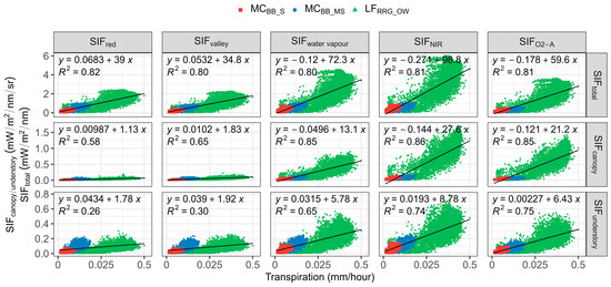
Figure 4.
Scatterplot of transpiration (T) against sun-induced chlorophyll fluorescence (SIF) emissions of selected SIF bands from total leaves, canopy, and understory components. All p-values < 0.05. SIFred is SIF emission at 685 nm; SIFvalley is 699 nm; SIFwater vapour is 720 nm; SIFNIR is 740 nm; SIFO2-A is 760 nm. SIFtotal is the total SIF emission at the leaf level, SIFcanopy is the SIF emission from the canopy, SIFunderstory is the SIF emission from understory vegetation.
It was apparent SIF–T relationships were stronger at the canopy level for all three sites, especially for the sparse forest (MCBB_S; Table 5). This suggests that the performance of SIF in predicting T was influenced by vegetation structure. When comparing the relationship of SIFcanopy and T to the relationship of SIFunderstory and T, R2 was higher at the canopy layer, implying canopy SIF could better explain T variations, and SIF–T correlations were considerably weakened when considering SIF emissions in the whole scene, including SIFunderstory.
3.1.3. Timeseries of SIF and T Comparison across All Sites
Two common SIF bands, SIFred and SIFNIR, were selected to assess seasonal trends within in situ measured T from June 2019 to May 2021 for MCBB_S, MCBB_MS, and LFRRG_OW (Figure 5). With increasing FVC, average values of both T and SIF emissions for red and NIR bands at LFRRG_OW were higher than low FVC sites (MCBB_S and MCBB_MS). For example, mean SIFNIR and T at the hourly scale for LFRRG_OW were 1.09 ± 0.48 mW m−2 nm−1 sr−1 and 0.33 ± 0.008 mm h−1, respectively, while mean SIFNIR and T at MCBB_S were 0.14 ± 0.06 mW m−2 nm−1 sr−1 and 0.005 ± 0.001 mm h−1, respectively. Rainfall in the hydrological year of 2019 (HY-2019, June 2019–May 2020) was lower than the hydrological year of 2020 (HY-2020, June 2020–May 2021) due to 2019 being the most extensive drought year on record [89], leading to slightly higher T in HY-2020 than HY-2019. Similarly, SIFNIR had larger values in HY-2020 than HY-2019. Both hourly SIFNIR and T had similar seasonal trends, peaking at the beginning of 2021 at all sites (Figure 5), demonstrating SIFNIR could track T variations and monitor tree water use trends. However, peaks of SIFNIR and T at MCBB_S in HY-2019 were inconsistent, with a lag of two months (Figure 5a) in SIFNIR, identified by determining the peak seasons of SIFNIR and T using singular spectrum analysis [81]. A sudden rise of T around May 2020 was not demonstrated in the SIFNIR data for this site.
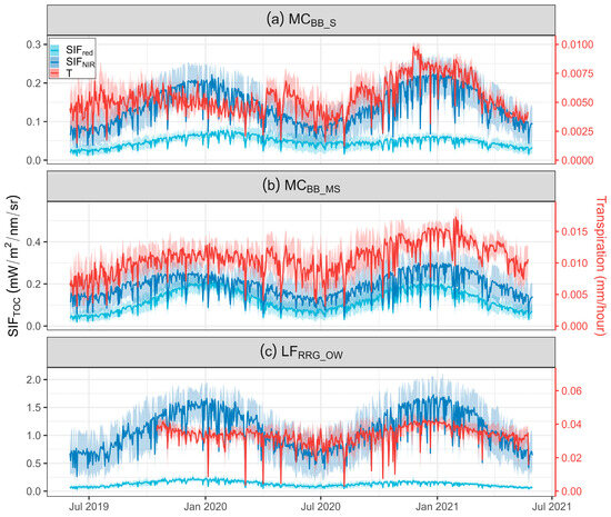
Figure 5.
Time series of sun-induced chlorophyll fluorescence (SIF) simulations (685 and 740 nm) and transpiration (T) measurements at (a) Mallee Cliffs E. largiflorens sparse site (MCBB_S), (b) Mallee Cliffs E. largiflorens moderately sparse site (MCBB_MS), and (c) Lindsay Forest E. camaldulensis open woodland site (LFRRG_OW).
During the wet season of 2020 (April–August), the value of T remained high compared to SIF, which exhibited less seasonality, particularly at LFRRG_OW (Figure 5c). Additionally, the range of T during peak times (i.e., January 2021) was narrow, implying daily fluctuations of T were restricted around periods of high T. Results of SIFNIR and SIFred, however, did not demonstrate similar trends, and the SIFred trend was quite depressed when compared to SIFNIR at LFRRG_OW (Figure 5c). The SIFred results display similar seasonal trends to SIFNIR at both MCBB_S and MCBB_MS.
To explore diurnal variation in photosynthetic activity and tree water use in these sparse open woodlands, mean diurnal patterns of SIF and T were investigated (Figure S3). Strong correlations between SIFNIR and T were observed at all sites (R2 = 0.96 for MCBB_S, R2 = 0.88 for MCBB_MS, and R2 = 0.96 for LFRRG_OW, all p-values < 0.05), while R2 > 0.84 for correlations between SIFred and T for all sites. In addition, a common pattern was found at all sites, with both SIF and T increasing in the morning, maintaining a steady state around noon, and declining during the afternoon. Transpiration peaked one hour earlier than SIF at MCBB_MS and MCBB_S, respectively. Both SIF and T peaked at 1200 h at LFRRG_OW, compared to T at lower FVC sites (MCBB_S and MCBB_MS), where the peak occurred at around 1100 h.
3.2. Influence of Environmental Factors on SIF–T Correlation
3.2.1. Influence of Soil Reflectance and LAI on SIF–T Correlations
There was no evidence that LAIu had a major influence on SIF–T relationships (Figure 6). When LAIu increased, the R2 between SIF and T increased slightly, suggesting the influence of LAIu on the SIF–T relationships was minimal. In addition, it was found that a weak SIF–T relationship existed in sparse forest. With the increase in canopy cover, SIF could explain more variations of T in moderately sparse forest. However, relationships between red SIF and T were degraded in open woodlands (Figure 6). Likewise, three classes of Rsoil were tested, and the R2 of T and SIF emissions for selected bands were slightly degraded (Figure S2). Hence, results suggested the forest background was not the main factor that impacts the ability of SIFred to predict T.
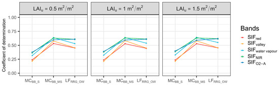
Figure 6.
Coefficient of determinations of correlations between sun-induced chlorophyll fluorescence (SIF) and transpiration (T) at the hourly scale with defined understory leaf area index (LAIu) for each site. MCBB_S is Mallee Cliffs E. largiflorens sparse site, MCBB_MS is Mallee Cliffs E. largiflorens moderately sparse site, and LFRRG_OW is Lindsay Forest E. camaldulensis open woodland site. SIFred is SIF emission at 685 nm; SIFvalley is 699 nm; SIFwater vapour is 720 nm; SIFNIR is 740 nm; SIFO2-A is 760 nm.
3.2.2. Influence of Canopy Leaf Area Index, Temperature, and Rainfall on SIF–T Correlations
Correlation between T and SIF emissions for selected bands under different LAI conditions were assessed (Figure 7), revealing that SIF was not significantly correlated with T when LAI was ≤0.4 m2 m−2 (i.e., sparse forest). However, correlations strengthened above this threshold. The R2 between SIF (SIFwater vapour, SIFNIR, and SIFO2-A) and T decreased slightly when LAI was >0.5 m2 m−2 and was highest between 0.4 m2 m−2 and 0.5 m2 m−2. For the three LAI classes, SIFO2-A had a higher predictive performance for sparse and open woodland, and SIFwater vapour for moderately sparse woodlands. Interestingly, SIFred had an overall higher predictive performance than SIFvalley for sparse forest, even with a very low R2 (0.14). This may indicate that more red SIF photons could escape from the canopy due to a low probability of photon absorption and collision during transmission.
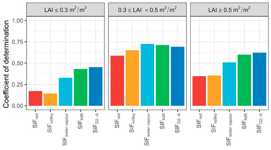
Figure 7.
Coefficient of determination of selected sun-induced chlorophyll fluorescence (SIF) bands and transpiration (T) at the hourly scale for various leaf area index (LAI) conditions. SIFred is SIF emission at 685 nm; SIFvalley is 699 nm; SIFwater vapour is 720 nm; SIFNIR is 740 nm; SIFO2-A is 760 nm.
Additionally, the correlation between SIF emissions and T was assessed using five temperature categories (Figure 8). Similar patterns were found between T and SIF (SIFwater vapour, SIFNIR, and SIFO2-A) for all sites with temperatures between 10 °C and >40 °C. However, the R2 between T and SIF emissions significantly degraded when the temperature rose above 30 °C for each site. With high-temperature conditions (temperature > 40 °C), almost all SIF bands could not predict T across the three sites (R2 < 0.25). Furthermore, it was noted that SIFred was mostly impacted by temperature, where increases in temperature from 10 to 40 °C decreased prediction performance from 50% to 24%. It is possible that LAI changes are related to temperature, with increasing LAI over the Austral spring—early summer, causing a degraded relationship between SIFred–T, as increases in leaf area mean more SIFred photons are absorbed during transmission. This requires further investigation.

Figure 8.
Coefficient of determination of sun-induced chlorophyll fluorescence (SIF) and transpiration (T) at the hourly scale with defined temperature (TEMP) categories. MCBB_S is Mallee Cliffs E. largiflorens sparse site, MCBB_MS is Mallee Cliffs E. largiflorens moderately sparse site, and LFRRG_OW is Lindsay Forest E. camaldulensis open woodland site. SIFred is SIF emission at 685 nm; SIFvalley is 699 nm; SIFwater vapour is 720 nm; SIFNIR is 740 nm; SIFO2-A is 760 nm. “*” denotes p-value is more than 0.05.
Various levels of rainfall led to statistically significant correlations between T and SIF emissions (Figure 9). When daily rainfall was under 3 mm, each site’s SIF–T relationship varied little with a moderate coefficient of variation. When rainfall was >10 mm, the SIF–T relationship degraded with increasing FVC, mostly due to rainfall interception increasing with FVC and affecting photon transmission. The SIF–T pattern for all sites was insignificant (R2 < 0.25) with daily rainfall above 10 mm. Overall, rainfall had little influence on SIF–T correlations as it was highly variable between rainfall intensity, FVC, and SIF band. It appeared SIFNIR and SIFwater vapour exhibited the highest SIF–T correlations across rainfall intensity and FVC.
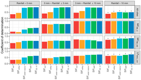
Figure 9.
Coefficient of determinations of sun-induced chlorophyll fluorescence (SIF) and transpiration (T) at the hourly scale with various daily rainfall (mm day−1) conditions. MCBB_S is Mallee Cliffs E. largiflorens sparse site, MCBB_MS is Mallee Cliffs E. largiflorens moderately sparse site, and LFRRG_OW is Lindsay Forest E. camaldulensis open woodland site. SIFred is SIF emission at 685 nm; SIFvalley is 699 nm; SIFwater vapour is 720 nm; SIFNIR is 740 nm; SIFO2-A is 760 nm. “*” denotes p-value is more than 0.05.
4. Discussion
This study assesses the ability of multiple SIF bands to explain T for open woodland environments with varying fractional vegetation cover. It was found that SIFNIR performed better than other bands and explained 93% of the variations in T at the monthly scale for open woodlands. The relationship between SIF and T was examined at various temporal resolutions and different environmental conditions. The SIF–T relationship strengthened as FVC increased, and this relationship remained unaffected with rising temperature and rainfall, except when the temperature surpassed 30 degrees or daily rainfall exceeded 10 mm. Additionally, understory and soil reflection had little influence on SIF’s ability to predict T. This study aims to improve understanding of the SIF–T relationship for open woodlands to contribute to accurate broadscale mapping of tree water use.
4.1. SIF Emission Performance in Explaining T Variation
It appears that SIFred had the weakest correlation with T compared with other SIF bands (Figure 3). Even though SIFred carries the information of PSII and aligns well with photosynthetic activity at the leaf scale [34], SIFred could not explain T variations in sparse woodlands due to small SIFred emission and re-absorption effects in this region. Similarly, when compared with a previous study of SIFred–T correlations in mature dense forest, it was determined that the ability of SIFred to predict T was not as strong as other SIF bands [36]. However, a moderate positive correlation between T and SIFtotal in the red band was found for sparse forests (R2 = 0.30, Table 5) as SIFtotal in the red band is computed from SIF emissions at the leaf level, which is not yet affected by the re-absorption effect. The fluorescence escape ratio (fesc = SIFTOC∙π/SIFtotal) also supports this phenomenon [47,90]. It is defined as the rate of observed SIF at the TOC [47] and used to examine the influence of vegetation structure on SIF photon transference. For sparse forests in this study, the value range of the fesc at the red band was from 0.02 to 0.11 (Figure S6), which was lower than that of dense forests (0.17–0.24) in previous studies [47,90,91]. This implies that only a small portion red SIF could be observed at the TOC for sparse forests. A possible explanation could be that low FVC leads to less SIF emissions. It is noted that the trees in this study (E. largiflorens and E. camaldulensis) possess vertical leaf inclination, which could be another factor causing low fesc, as more photons transfer horizontally rather than escape vertically to the sky. Hence, it is clear that the re-absorption effect significantly impacted SIFred at TOC in this study. Additionally, SIFred performance for T predictions increased by 31% from sparse to moderately sparse forest for hourly data but then declined by 13% for open woodland (Table 4). While there was an increasing SIFred emission with increasing FVC, the reabsorption effect impacted SIFred photon transmission, indicating a possible threshold limiting SIFred performance in predicting T with increasing FVC. Additionally, red region SIFvalley-T performance appeared better than SIFred, although SIFvalley was less effective in predicting T variation with varying environmental factors, such as high temperature and rainfall.
Whilst SIFwater vapour showed an improved relationship with T for moderately sparse forests, (MCBB_MS, R2 = 0.58), the performance of SIFwater vapour in predicting T was weaker when compared to SIFNIR and SIFO2-A for high FVC (LFRRG_OW). This outcome is contrary to previous studies, suggesting that SIFwater vapour has the highest R2 for T estimation for dense and mature forests [36]. Furthermore, it is difficult to retrieve SIF from the water vapour region due to spatial variability of the water vapour band being influenced by temperature and humidity [92].
In our study, SIFNIR produced the strongest correlation with T at MCBB_S and LFRRG_OW, generating a universal model to predict T for various FVC conditions. Furthermore, SIFNIR was more sensitive to changing temperature and precipitation than other SIF bands and was less influenced by the re-absorption effect [93]. Most studies have established that SIFNIR was highly correlated with photosynthetic activity under various environmental conditions [94,95], such as extreme heat and water stress. Hence, SIFNIR is the most reliable band in predicting T for sparse forests. Similarly, SIFO2-A displayed a similar performance to SIFNIR in predicting T for sparse forests.
It is noted that SIFO2-A is widely retrieved from the satellite data (GOME-2 and OCO-2) and field measurement. The strongest correlation between SIFO2-A and T was exhibited at the high FVC site (LFRRG_OW) at both daily and monthly scales (R2 = 0.55 and 0.73 for daily and monthly, respectively; Table 4). These results are consistent with previous research demonstrating the effectiveness of SIFO2-A in estimating tree water use (T) using remote sensing data [38,96]. Hence, SIFO2-A might be the best replacement for SIFNIR for predicting T from space, which is more difficult to retrieve.
4.2. Further Research
Although a universal model was found using SIF to predict T for sparse woodlands, limitations of this research need to be addressed. Firstly, the EF-matrix was retrieved from remote sensing VI products and interpolated to the daily scale. However, the EF-matrix varies with environmental factors [97]; for example, CO2 density or temperature. Currently, the Fluspect-B model is incapable of simulating the EF-matrix with environmental factors. Hence, modelling the EF-matrix with real-time environmental factors could improve the accuracy of SIF simulations and better estimate T at finer temporal scales.
A mismatch in peak timing between SIFNIR and T was observed in MCBB_S (Figure 5) where transpiration reached a peak two months earlier than SIF in HY-2019, and SIF did not respond to a spike in T in during the dry season at this site. Conversely, both SIF and T demonstrated simultaneous declines on cloudy days. These results might be due to FluorFLiES simulated SIF being driven by incoming radiation and the EF-matrix. For example, the seasonal variation of radiation might have led SIF to peak two months later. The SIF emission reduces on cloudy days where tree T is reduced in relation to reduced evaporative demand [98,99]. In addition, the EF-matrix was retrieved from VIs, which are less sensitive to water stress [100]. In summary, improving the method of retrieving the EF-matrix would be beneficial for understanding SIF’s ability to predict tree water use.
This study does, however, provide some feasible future applications, such as improving the understanding of tree water use for floodplain vegetation by incorporating SIF. Since direct monitoring of tree water use from space is not possible, SIF is an effective tool for estimating T at various spatial and temporal scales. The strong relationship between SIF and T identified in this study can assist water managers in developing effective strategies for water resource allocation and maintaining ecosystem biodiversity in floodplains. Furthermore, SIF may benefit the assessment of carbon sequestration for floodplain trees [101]. As SIF serves as a link between the carbon and water cycles, it would be useful to study how tree water use impacts carbon sinks in floodplain environments. A further application is to produce an improved spatial ET product. Currently, remote sensing ET products rely on a complex energy balance and mass transfer model with multiple environmental data [102]. This study helps to improve SIF performance in predicting T, and further improved estimation of ET. In addition, the advanced SIF satellite, the Fluorescence Explorer, will be launched in 2025, carrying a high-resolution fluorescence sensor providing SIF data with a 300 m spatial resolution [103]. Improved spatial resolution form this SIF satellite will enhance global SIF monitoring in the NIR band, improving future global ET estimation.
5. Conclusions
A 3D model, FluorFLiES, was implemented to simulate hourly SIF for three floodplain sparse forests with different FVC, evaluating THE performance of five specific SIF bands in predicting T spatially and temporally. Previous studies on the SIF–T relationship focused on dense forests and assumed vegetation was homogeneously distributed, but this work used a 3D model to present accurate vegetation structure and evaluated how sparse forest structure impacts SIF–T within various environmental conditions. This study has demonstrated that a universal model can be used to predict T using SIFNIR, which was able to explain 85% of T variation for sparse woodlands at the hourly scale. With upscaling to monthly data, the R2 of SIFNIR–T correlations increased to 93%. When removing the reabsorption effect at the leaf scale, red SIF performance in predicting T increased by 24%. Partitioning the SIF signal to the canopy scale, SIFNIR‘s ability to predict T increased by 5%. Sensitivity analysis of understory parameters was conducted with variations of LAIu and Rsoil, highlighting that they did not strongly impact the relationship between SIF and T. Additionally, a weakened SIF–T correlation (R2 < 0.25) was confirmed with high temperatures and heavy daily rainfall, helping us understand this relationship under extreme weather conditions. Study results have the ability to improve T estimation by using SIF, bridging several knowledge gaps in understanding the relationship between tree transpiration and multiple SIF bands. The novelty of this study includes the availability of robust in situ data to compare SIF modelling results against. It is anticipated that future scenario modelling of open woodland water use under differing climate models can now be undertaken to provide more confidence in water use estimates to inform water accounting and determination of sustainable levels of hydrological extraction across the MDB, where open woodlands are the dominant vegetation community. Furthermore, this method is applicable more broadly to river basins across the world.
Supplementary Materials
The following supporting information can be downloaded at: https://www.mdpi.com/article/10.3390/rs16010143/s1, Model validation; Figure S1: Scatter plot of the estimation of transpiration using SIF versus measured T; Figure S2: Coefficient of determinations of correlations between T and SIF emissions at the hourly scale with defined soil reflectance; Figure S3: Mean diurnal patterns of SIF emission; Figure S4: Diurnal photosynthetic active radiation for each site; Figure S5: FluorFLiES model simulated SIF at 740 nm compared with TROPOMI SIF; Figure S6: Violine plots of the escape ratio of SIF emission; Figure S7 Correlation between Cab and the chlorophyll index; Figure S8: Soil reflectance value range; Table S1 Full names of acronyms [104,105].
Author Contributions
Conceptualization, S.G. and T.M.D.; methodology, S.G., W.W., X.M. and T.M.D.; software, S.G.; validation, S.G.; formal analysis, S.G.; investigation, S.G. and T.M.D.; resources, S.G.; data curation, S.G.; writing—original draft preparation, S.G., W.W., X.M. and T.M.D.; writing—review and editing, S.G. and T.M.D.; visualization, S.G.; supervision, T.M.D.; project administration, T.M.D.; funding acquisition, T.M.D. All authors have read and agreed to the published version of the manuscript.
Funding
This research was funded by the Murray–Darling Basin Authority.
Data Availability Statement
The data presented in this study are available upon request from the corresponding author.
Acknowledgments
We would like to acknowledge funding contributions from the Murray–Darling Basin Authority, which have contributed to this research. The research product of PAR (produced from Himawari-8) that was used in this paper was supplied by the P-Tree System, Japan Aerospace Exploration Agency (JAXA). We are grateful to Micah Davies, Sophie Gilbey, Ruan Gannon, Adam McKeown, and Jess Thompson for collecting data.
Conflicts of Interest
The authors declare no conflicts of interest.
References
- Cui, Y.; Chen, X.; Gao, J.; Yan, B.; Tang, G.; Hong, Y. Global Water Cycle and Remote Sensing Big Data: Overview, Challenge, and Opportunities. Big Earth Data 2018, 2, 282–297. [Google Scholar] [CrossRef]
- Huntington, T.G. Evidence for Intensification of the Global Water Cycle: Review and Synthesis. J. Hydrol. 2006, 319, 83–95. [Google Scholar] [CrossRef]
- Mehta, V.M.; DeCandis, A.J.; Mehta, A.V. Remote-Sensing-Based Estimates of the Fundamental Global Water Cycle: Annual Cycle. J. Geophys. Res. Atmos. 2005, 110, 1–14. [Google Scholar] [CrossRef]
- Abbott, B.W.; Bishop, K.; Zarnetske, J.P.; Minaudo, C.; Chapin, F.S.; Krause, S.; Hannah, D.M.; Conner, L.; Ellison, D.; Godsey, S.E.; et al. Human Domination of the Global Water Cycle Absent from Depictions and Perceptions. Nat. Geosci. 2019, 12, 533–540. [Google Scholar] [CrossRef]
- Haddeland, I.; Heinke, J.; Biemans, H.; Eisner, S.; Flörke, M.; Hanasaki, N.; Konzmann, M.; Ludwig, F.; Masaki, Y.; Schewe, J.; et al. Global Water Resources Affected by Human Interventions and Climate Change. Proc. Natl. Acad. Sci. USA 2013, 111, 3251–3256. [Google Scholar] [CrossRef] [PubMed]
- Avand, M.; Moradi, H.; lasboyee, M.R. Using Machine Learning Models, Remote Sensing, and GIS to Investigate the Effects of Changing Climates and Land Uses on Flood Probability. J. Hydrol. 2021, 595, 125663. [Google Scholar] [CrossRef]
- West, H.; Quinn, N.; Horswell, M. Remote Sensing for Drought Monitoring & Impact Assessment: Progress, Past Challenges and Future Opportunities. Remote Sens. Environ. 2019, 232, 111291. [Google Scholar] [CrossRef]
- Miguez-Macho, G.; Fan, Y. The Role of Groundwater in the Amazon Water Cycle: 2. Influence on Seasonal Soil Moisture and Evapotranspiration. J. Geophys. Res. Atmos. 2012, 117, D15. [Google Scholar] [CrossRef]
- Mu, Q.; Heinsch, F.A.; Zhao, M.; Running, S.W. Development of a Global Evapotranspiration Algorithm Based on MODIS and Global Meteorology Data. Remote Sens. Environ. 2007, 111, 519–536. [Google Scholar] [CrossRef]
- Schlesinger, W.H.; Jasechko, S. Transpiration in the Global Water Cycle. Agric. For. Meteorol. 2014, 189–190, 115–117. [Google Scholar] [CrossRef]
- Jasechko, S.; Sharp, Z.D.; Gibson, J.J.; Birks, S.J.; Yi, Y.; Fawcett, P.J. Terrestrial Water Fluxes Dominated by Transpiration. Nature 2013, 496, 347–350. [Google Scholar] [CrossRef] [PubMed]
- Tuzet, A.J. Stomatal Conductance, Photosynthesis, and Transpiration, Modeling. In Encyclopedia of Agrophysics; Encyclopedia of Earth Sciences Series; Springer: Berlin/Heidelberg, Germany, 2011; Part 4; pp. 855–858. [Google Scholar] [CrossRef]
- Moore, D.J.P.; Hu, J.; Sacks, W.J.; Schimel, D.S.; Monson, R.K. Estimating Transpiration and the Sensitivity of Carbon Uptake to Water Availability in a Subalpine Forest Using a Simple Ecosystem Process Model Informed by Measured Net CO2 and H2O Fluxes. Agric. For. Meteorol. 2008, 148, 1467–1477. [Google Scholar] [CrossRef]
- Boegh, E.; Soegaard, H.; Hanan, N.; Kabat, P.; Lesch, L. A Remote Sensing Study of the NDVI–Ts Relationship and the Transpiration from Sparse Vegetation in the Sahel Based on High-Resolution Satellite Data. Remote Sens. Environ. 1999, 69, 224–240. [Google Scholar] [CrossRef]
- Pagán, B.R.; Maes, W.H.; Gentine, P.; Martens, B.; Miralles, D.G. Exploring the Potential of Satellite Solar-Induced Fluorescence to Constrain Global Transpiration Estimates. Remote Sens. 2019, 11, 413. [Google Scholar] [CrossRef]
- Monteith, J.L. Evaporation and Environment. Symp. Soc. Exp. Biol. 1965, 19, 205–234. [Google Scholar] [PubMed]
- Priestley, C.H.B.; Taylor, R.J. On the Assessment of Surface Heat Flux and Evaporation Using Large-Scale Parameters. Mon. Weather Rev. 1972, 100, 81–92. [Google Scholar] [CrossRef]
- Wutzler, T.; Lucas-Moffat, A.; Migliavacca, M.; Knauer, J.; Sickel, K.; Šigut, L.; Menzer, O.; Reichstein, M. Basic and Extensible Post-Processing of Eddy Covariance Flux Data with REddyProc. Biogeosciences 2018, 15, 5015–5030. [Google Scholar] [CrossRef]
- Doody, T.M.; Colloff, M.J.; Davies, M.; Koul, V.; Benyon, R.G.; Nagler, P.L. Quantifying Water Requirements of Riparian River Red Gum (Eucalyptus Camaldulensis) in the Murray–Darling Basin, Australia—Implications for the Management of Environmental Flows. Ecohydrology 2015, 8, 1471–1487. [Google Scholar] [CrossRef]
- Steppe, K.; De Pauw, D.J.W.; Doody, T.M.; Teskey, R.O. A Comparison of Sap Flux Density Using Thermal Dissipation, Heat Pulse Velocity and Heat Field Deformation Methods. Agric. For. Meteorol. 2010, 150, 1046–1056. [Google Scholar] [CrossRef]
- Zhang, H.; Simmonds, L.P.; Morison, J.I.L.L.; Payne, D. Estimation of Transpiration by Single Trees: Comparison of Sap Flow Measurements with a Combination Equation. Agric. For. Meteorol. 1997, 87, 155–169. [Google Scholar] [CrossRef]
- Nagler, P.; Jetton, A.; Fleming, J.; Didan, K.; Glenn, E.; Erker, J.; Morino, K.; Milliken, J.; Gloss, S. Evapotranspiration in a Cottonwood (Populus fremontii) Restoration Plantation Estimated by Sap Flow and Remote Sensing Methods. Agric. For. Meteorol. 2007, 144, 95–110. [Google Scholar] [CrossRef]
- Jonard, F.; De Cannière, S.; Brüggemann, N.; Gentine, P.; Short Gianotti, D.J.; Lobet, G.; Miralles, D.G.; Montzka, C.; Pagán, B.R.; Rascher, U.; et al. Value of Sun-Induced Chlorophyll Fluorescence for Quantifying Hydrological States and Fluxes: Current Status and Challenges. Agric. For. Meteorol. 2020, 291, 108088. [Google Scholar] [CrossRef]
- Sun, Y.; Fu, R.; Dickinson, R.; Joiner, J.; Frankenberg, C.; Gu, L.; Xia, Y.; Fernando, N. Drought Onset Mechanisms Revealed by Satellite Solar-Induced Chlorophyll Fluorescence: Insights from Two Contrasting Extreme Events. J. Geophys. Res. Biogeosci. 2015, 120, 2427–2440. [Google Scholar] [CrossRef]
- Ma, X.; Huete, A.; Cleverly, J.; Eamus, D.; Chevallier, F.; Joiner, J.; Poulter, B.; Zhang, Y.; Guanter, L.; Meyer, W.; et al. Drought Rapidly Diminishes the Large Net CO2 Uptake in 2011 over Semi-Arid Australia. Sci. Rep. 2016, 6, 37747. [Google Scholar] [CrossRef] [PubMed]
- MacBean, N.; Maignan, F.; Bacour, C.; Lewis, P.; Peylin, P.; Guanter, L.; Köhler, P.; Gómez-Dans, J.; Disney, M. Strong Constraint on Modelled Global Carbon Uptake Using Solar-Induced Chlorophyll Fluorescence Data. Sci. Rep. 2018, 8, 1973. [Google Scholar] [CrossRef] [PubMed]
- Mohammed, G.H.; Colombo, R.; Middleton, E.M.; Rascher, U.; van der Tol, C.; Nedbal, L.; Goulas, Y.; Pérez-Priego, O.; Damm, A.; Meroni, M.; et al. Remote Sensing of Solar-Induced Chlorophyll Fluorescence (SIF) in Vegetation: 50 years of Progress. Remote Sens. Environ. 2019, 231, 111177. [Google Scholar] [CrossRef] [PubMed]
- Palombi, L.; Cecchi, G.; Lognoli, D.; Raimondi, V.; Toci, G.; Agati, G. A Retrieval Algorithm to Evaluate the Photosystem I and Photosystem II Spectral Contributions to Leaf Chlorophyll Fluorescence at Physiological Temperatures. Photosynth. Res. 2011, 108, 225–239. [Google Scholar] [CrossRef]
- Porcar-Castell, A.; Malenovský, Z.; Magney, T.; Van Wittenberghe, S.; Fernández-Marín, B.; Maignan, F.; Zhang, Y.; Maseyk, K.; Atherton, J.; Albert, L.P.; et al. Chlorophyll a Fluorescence Illuminates a Path Connecting Plant Molecular Biology to Earth-System Science. Nat. Plants 2021, 7, 998–1009. [Google Scholar] [CrossRef]
- Franck, F.; Juneau, P.; Popovic, R. Resolution of the Photosystem I and Photosystem II Contributions to Chlorophyll Fluorescence of Intact Leaves at Room Temperature. Biochim. Biophys. Acta Bioenerg. 2002, 1556, 239–246. [Google Scholar] [CrossRef]
- Wientjes, E.; Philippi, J.; Borst, J.W.; van Amerongen, H. Imaging the Photosystem I/Photosystem II Chlorophyll Ratio inside the Leaf. Biochim. Biophys. Acta-Bioenerg. 2017, 1858, 259–265. [Google Scholar] [CrossRef]
- Verrelst, J.; Rivera, J.P.; Gitelson, A.; Delegido, J.; Moreno, J.; Camps-Valls, G. Spectral Band Selection for Vegetation Properties Retrieval Using Gaussian Processes Regression. Int. J. Appl. Earth Obs. Geoinf. 2016, 52, 554–567. [Google Scholar] [CrossRef]
- Li, D.; Wu, S.; Liu, L.; Zhang, Y.; Li, S. Vulnerability of the Global Terrestrial Ecosystems to Climate Change. Glob. Chang. Biol. 2018, 24, 4095–4106. [Google Scholar] [CrossRef] [PubMed]
- Magney, T.S.; Frankenberg, C.; Köhler, P.; North, G.; Davis, T.S.; Dold, C.; Dutta, D.; Fisher, J.B.; Grossmann, K.; Harrington, A.; et al. Disentangling Changes in the Spectral Shape of Chlorophyll Fluorescence: Implications for Remote Sensing of Photosynthesis. J. Geophys. Res. Biogeosci. 2019, 124, 1491–1507. [Google Scholar] [CrossRef]
- Sun, Y.; Frankenberg, C.; Wood, J.D.; Schimel, D.S.; Jung, M.; Guanter, L.; Drewry, D.T.; Verma, M.; Porcar-Castell, A.; Griffis, T.J. OCO-2 Advances Photosynthesis Observation from Space via Solar-Induced Chlorophyll Fluorescence. Science 2017, 358, eaam5747. [Google Scholar] [CrossRef] [PubMed]
- Lu, X.; Liu, Z.; An, S.; Miralles, D.G.; Maes, W.; Liu, Y.; Tang, J. Potential of Solar-Induced Chlorophyll Fluorescence to Estimate Transpiration in a Temperate Forest. Agric. For. Meteorol. 2018, 252, 75–87. [Google Scholar] [CrossRef]
- Damm, A.; Roethlin, S.; Fritsche, L. Towards Advanced Retrievals of Plant Transpiration Using Suninduced Chlorophyll Fluorescence: First Considerations. In Proceedings of the International Geoscience and Remote Sensing Symposium (IGARSS), Valencia, Spain, 22–27 July 2018; Institute of Electrical and Electronics Engineers Inc.: New York, NY, USA, 2018; pp. 5983–5986. [Google Scholar]
- Maes, W.H.; Pagán, B.R.; Martens, B.; Gentine, P.; Guanter, L.; Steppe, K.; Verhoest, N.E.C.; Dorigo, W.; Li, X.; Xiao, J.; et al. Sun-Induced Fluorescence Closely Linked to Ecosystem Transpiration as Evidenced by Satellite Data and Radiative Transfer Models. Remote Sens. Environ. 2020, 249, 112030. [Google Scholar] [CrossRef]
- Shan, N.; Ju, W.; Migliavacca, M.; Martini, D.; Guanter, L.; Chen, J.; Goulas, Y.; Zhang, Y. Modeling Canopy Conductance and Transpiration from Solar-Induced Chlorophyll Fluorescence. Agric. For. Meteorol. 2019, 268, 189–201. [Google Scholar] [CrossRef]
- Ahmed, K.R.; Paul-Limoges, E.; Rascher, U.; Hanus, J.; Miglietta, F.; Colombo, R.; Peressotti, A.; Genangeli, A.; Damm, A. Empirical Insights on the Use of Sun-Induced Chlorophyll Fluorescence to Estimate Short-Term Changes in Crop Transpiration under Controlled Water Limitation. ISPRS J. Photogramm. Remote Sens. 2023, 203, 71–85. [Google Scholar] [CrossRef]
- Liu, Y.; Zhang, Y.; Shan, N.; Zhang, Z.; Wei, Z. Global Assessment of Partitioning Transpiration from Evapotranspiration Based on Satellite Solar-Induced Chlorophyll Fluorescence Data. J. Hydrol. 2022, 612, 128044. [Google Scholar] [CrossRef]
- Gao, S.; Huete, A.; Kobayashi, H.; Doody, T.M.; Liu, W.; Wang, Y.; Zhang, Y.; Lu, X. Simulation of Solar-Induced Chlorophyll Fluorescence in a Heterogeneous Forest Using 3-D Radiative Transfer Modelling and Airborne LiDAR. ISPRS J. Photogramm. Remote Sens. 2022, 191, 1–17. [Google Scholar] [CrossRef]
- Zeng, Y.; Badgley, G.; Chen, M.; Li, J.; Anderegg, L.D.L.; Kornfeld, A.; Liu, Q.; Xu, B.; Yang, B.; Yan, K.; et al. A Radiative Transfer Model for Solar Induced Fluorescence Using Spectral Invariants Theory. Remote Sens. Environ. 2020, 240, 111678. [Google Scholar] [CrossRef]
- Hernández-Clemente, R.; North, P.R.J.; Hornero, A.; Zarco-Tejada, P.J. Assessing the Effects of Forest Health on Sun-Induced Chlorophyll Fluorescence Using the FluorFLIGHT 3-D Radiative Transfer Model to Account for Forest Structure. Remote Sens. Environ. 2017, 193, 165–179. [Google Scholar] [CrossRef]
- Liu, W.; Atherton, J.; Mõttus, M.; Gastellu-Etchegorry, J.P.; Malenovský, Z.; Raumonen, P.; Åkerblom, M.; Mäkipää, R.; Porcar-Castell, A. Simulating Solar-Induced Chlorophyll Fluorescence in a Boreal Forest Stand Reconstructed from Terrestrial Laser Scanning Measurements. Remote Sens. Environ. 2019, 232, 111274. [Google Scholar] [CrossRef]
- Zhao, F.; Dai, X.; Verhoef, W.; Guo, Y.; van der Tol, C.; Li, Y.; Huang, Y. FluorWPS: A Monte Carlo Ray-Tracing Model to Compute Sun-Induced Chlorophyll Fluorescence of Three-Dimensional Canopy. Remote Sens. Environ. 2016, 187, 385–399. [Google Scholar] [CrossRef]
- Lu, X.; Liu, Z.; Zhao, F.; Tang, J. Comparison of Total Emitted Solar-Induced Chlorophyll Fluorescence (SIF) and Top-of-Canopy (TOC) SIF in Estimating Photosynthesis. Remote Sens. Environ. 2020, 251, 112083. [Google Scholar] [CrossRef]
- Chu, H.; Luo, X.; Ouyang, Z.; Chan, W.S.; Dengel, S.; Biraud, S.C.; Torn, M.S.; Metzger, S.; Kumar, J.; Arain, M.A.; et al. Representativeness of Eddy-Covariance Flux Footprints for Areas Surrounding AmeriFlux Sites. Agric. For. Meteorol. 2021, 301–302, 108350. [Google Scholar] [CrossRef]
- Doody, T.M.; Gehrig, S.L.; Vervoort, R.W.; Colloff, M.J.; Doble, R. Determining Water Requirements for Black Box (Eucalyptus Largiflorens) Floodplain Woodlands of High Conservation Value Using Drip-Irrigation. Hydrol. Process 2021, 35, e14291. [Google Scholar] [CrossRef]
- Doody, T.M.; Gao, S.; Vervoort, W.; Pritchard, J.; Davies, M.; Nolan, M.; Nagler, P.L. A River Basin Spatial Model to Quantitively Advance Understanding of Riverine Tree Response Dynamics to Water Availability and Hydrological Management. J. Environ. Manag. 2023, 332, 117393. [Google Scholar] [CrossRef]
- Doody, T.M.; Benyon, R.G.; Gao, S. Fine Scale 20-Year Timeseries of Plantation Forest Evapotranspiration for the Lower Limestone Coast. Hydrol. Process 2023, 37, e14836. [Google Scholar] [CrossRef]
- ABS Water and the Murray Darling Basin—A Statistical Profile, 2000-01 to 2005-06; Australian Bureau of Statistics: Canberra, Australia, 2008.
- Van Dijk, A.I.J.M.; Beck, H.E.; Crosbie, R.S.; De Jeu, R.A.M.; Liu, Y.Y.; Podger, G.M.; Timbal, B.; Viney, N.R. The Millennium Drought in Southeast Australia (2001–2009): Natural and Human Causes and Implications for Water Resources, Ecosystems, Economy, and Society. Water Resour. Res. 2013, 49, 1040–1057. [Google Scholar] [CrossRef]
- Roberts, J.; Marston, F. Water Regime for Wetland and Floodplain Plants A Source Book for the Murray–Darling Basin; National Water Commission: Canberra, Australia, 2011. [Google Scholar]
- Overton, I.C.; Jolly, I.D. Integrated Studies of Floodplain Vegetation Health, Saline Groundwater and Flooding on the Chowilla Floodplain South Australia.; CSIRO Land and Water: Adelaide, Australia, 2004. [Google Scholar]
- Hart, B.; Walker, G.; Katupitiya, A.; Doolan, J. Salinity Management in the Murray–Darling Basin, Australia. Water 2020, 12, 1829. [Google Scholar] [CrossRef]
- Doody, T.M.; Benger, S.N.; Pritchard, J.L.; Overton, I.C.; Doody, T.M.; Benger, S.N.; Pritchard, J.L.; Overton, I.C. Ecological Response of Eucalyptus Camaldulensis (River Red Gum) to Extended Drought and Flooding along the River Murray, South Australia (1997–2011) and Implications for Environmental Flow Management. Mar. Freshw. Res. 2014, 65, 1082–1093. [Google Scholar] [CrossRef]
- Laattoe, T.; Werner, A.D.; Woods, J.A.; Cartwright, I. Terrestrial Freshwater Lenses: Unexplored Subterranean Oases. J. Hydrol. 2017, 553, 501–507. [Google Scholar] [CrossRef]
- Benyon, R.G.; Doody, T.M. Water Use by Tree Plantations in South East South Australia; CSIRO Forestry and Forest Products: Mt. Gambier, Australia, 2004. [Google Scholar]
- Burgess, S.S.O.; Adams, M.A.; Turner, N.C.; Beverly, C.R.; Ong, C.K.; Khan, A.A.H.; Bleby, T.M. An Improved Heat Pulse Method to Measure Low and Reverse Rates of Sap Flow in Woody Plants. Tree Physiol. 2001, 21, 589–598. [Google Scholar] [CrossRef] [PubMed]
- Dubayah, R.O.; Drake, J.B. Lidar Remote Sensing for Forestry; Oxford Academic: Oxford, UK, 2000; Volume 98. [Google Scholar]
- Frouin, R.; Murakami, H. Estimating Photosynthetically Available Radiation at the Ocean Surface from ADEOS-II Global Imager Data. J. Oceanogr. 2007, 63, 493–503. [Google Scholar] [CrossRef]
- Huete, A.; Didan, K.; Miura, T.; Rodriguez, E.P.; Gao, X.; Ferreira, L.G. Overview of the Radiometric and Biophysical Performance of the MODIS Vegetation Indices. Remote Sens. Environ. 2002, 83, 195–213. [Google Scholar] [CrossRef]
- Alexandrov, T.; Bianconcini, S.; Dagum, E.B.; Maass, P.; McElroy, T.S. A Review of Some Modern Approaches to the Problem of Trend Extraction. Econ. Rev. 2012, 31, 593–624. [Google Scholar] [CrossRef]
- Chen, J.M.; Rich, P.M.; Gower, S.T.; Norman, J.M.; Plummer, S. Leaf Area Index of Boreal Forests: Theory, Techniques, and Measurements. J. Geophys. Res. Atmos. 1997, 102, 29429–29443. [Google Scholar] [CrossRef]
- Putzenlechner, B.; Castro, S.; Kiese, R.; Ludwig, R.; Marzahn, P.; Sharp, I.; Sanchez-Azofeifa, A. Validation of Sentinel-2 FAPAR Products Using Ground Observations across Three Forest Ecosystems. Remote Sens. Environ. 2019, 232, 111310. [Google Scholar] [CrossRef]
- Weiss, M.; Baret, F.; Jay, S. S2ToolBox Level 2 Products: LAI, FAPAR, FCOVER, Version 2.0; Institut National de la Recherche Agronomique (INRA): Avignon, France, 2020. [Google Scholar]
- Kobayashi, H.; Iwabuchi, H. A Coupled 1-D Atmosphere and 3-D Canopy Radiative Transfer Model for Canopy Reflectance, Light Environment, and Photosynthesis Simulation in a Heterogeneous Landscape. Remote Sens. Environ. 2008, 112, 173–185. [Google Scholar] [CrossRef]
- Kobayashi, H.; Delbart, N.; Suzuki, R.; Kushida, K. A Satellite-Based Method for Monitoring Seasonality in the Overstory Leaf Area Index of Siberian Larch Forest. J. Geophys. Res. Biogeosci. 2010, 115, 1002. [Google Scholar] [CrossRef]
- Wu, J.; Kobayashi, H.; Stark, S.C.; Meng, R.; Guan, K.; Tran, N.N.; Gao, S.; Yang, W.; Restrepo-Coupe, N.; Miura, T.; et al. Biological Processes Dominate Seasonality of Remotely Sensed Canopy Greenness in an Amazon Evergreen Forest. New Phytol. 2018, 217, 1507–1520. [Google Scholar] [CrossRef] [PubMed]
- Kobayashi, H.; Baldocchi, D.D.; Ryu, Y.; Chen, Q.; Ma, S.; Osuna, J.L.; Ustin, S.L. Modeling Energy and Carbon Fluxes in a Heterogeneous Oak Woodland: A Three-Dimensional Approach. Agric. For. Meteorol. 2012, 152, 83–100. [Google Scholar] [CrossRef]
- Köhler, P.; Guanter, L.; Kobayashi, H.; Walther, S.; Yang, W. Assessing the Potential of Sun-Induced Fluorescence and the Canopy Scattering Coefficient to Track Large-Scale Vegetation Dynamics in Amazon Forests. Remote Sens. Environ. 2018, 204, 769–785. [Google Scholar] [CrossRef]
- Boehm, H.D.V.; Liesenberg, V.; Limin, S.H. Multi-Temporal Airborne LiDAR-Survey and Field Measurements of Tropical Peat Swamp Forest to Monitor Changes. IEEE J. Sel. Top. Appl. Earth Obs. Remote Sens. 2013, 6, 1524–1530. [Google Scholar] [CrossRef]
- Plowright, A. ForestTools: Analyzing Remotely Sensed Forest Data. In R Package, Version 0.1; R Core Team: Vienna, Austria, 2017; Volume 5. [Google Scholar]
- Beucher, S.; Meyer, F. The Morphological Approach to Segmentation: The Watershed Transformation. Math. Morphol. Image Process. 1993, 34, 433–481. [Google Scholar]
- Gao, S.; Castellazzi, P.; Vervoort, R.W.; Doody, T.M. Fine Scale Mapping of Fractional Tree Canopy Cover to Support River Basin Management. Hydrol. Process 2021, 35, e14156. [Google Scholar] [CrossRef]
- Pisek, J.; Adamson, K. Dataset of Leaf Inclination Angles for 71 Different Eucalyptus Species. Data Brief. 2020, 33, 106391. [Google Scholar] [CrossRef]
- Lu, H.; Raupach, M.R.; McVicar, T.R.; Barrett, D.J. Decomposition of Vegetation Cover into Woody and Herbaceous Components Using AVHRR NDVI Time Series. Remote Sens. Environ. 2003, 86, 1–18. [Google Scholar] [CrossRef]
- Ma, X.; Huete, A.; Moore, C.E.; Cleverly, J.; Hutley, L.B.; Beringer, J.; Leng, S.; Xie, Z.; Yu, Q.; Eamus, D. Spatiotemporal Partitioning of Savanna Plant Functional Type Productivity along NATT. Remote Sens. Environ. 2020, 246, 111855. [Google Scholar] [CrossRef]
- Zhuang, W.; Shi, H.; Ma, X.; Cleverly, J.; Beringer, J.; Zhang, Y.; He, J.; Eamus, D.; Yu, Q. Improving Estimation of Seasonal Evapotranspiration in Australian Tropical Savannas Using a Flexible Drought Index. Agric. For. Meteorol. 2020, 295, 108203. [Google Scholar] [CrossRef]
- Ma, X.; Huete, A.; Yu, Q.; Coupe, N.R.; Davies, K.; Broich, M.; Ratana, P.; Beringer, J.; Hutley, L.B.; Cleverly, J.; et al. Spatial Patterns and Temporal Dynamics in Savanna Vegetation Phenology across the North Australian Tropical Transect. Remote Sens. Environ. 2013, 139, 97–115. [Google Scholar] [CrossRef]
- Wei, S.; Yin, T.; Dissegna, M.A.; Whittle, A.J.; Ow, G.L.F.; Yusof, M.L.M.; Lauret, N.; Gastellu-Etchegorry, J.P. An Assessment Study of Three Indirect Methods for Estimating Leaf Area Density and Leaf Area Index of Individual Trees. Agric. For. Meteorol. 2020, 292–293, 108101. [Google Scholar] [CrossRef]
- Feret, J.-B.; François, C.; Asner, G.P.; Gitelson, A.A.; Martin, R.E.; Bidel, L.P.R.; Ustin, S.L.; Le Maire, G.; Jacquemoud, S. PROSPECT-4 and 5: Advances in the Leaf Optical Properties Model Separating Photosynthetic Pigments. Remote Sens. Environ. 2008, 112, 3030–3043. [Google Scholar] [CrossRef]
- Vilfan, N.; van der Tol, C.; Muller, O.; Rascher, U.; Verhoef, W. Fluspect-B: A Model for Leaf Fluorescence, Reflectance and Transmittance Spectra. Remote Sens. Environ. 2016, 186, 596–615. [Google Scholar] [CrossRef]
- Combal, B.; Baret, F.; Weiss, M.; Trubuil, A.; Macé, D.; Pragnère, A.; Myneni, R.; Knyazikhin, Y.; Wang, L. Retrieval of Canopy Biophysical Variables from Bidirectional Reflectance: Using Prior Information to Solve the Ill-Posed Inverse Problem. Remote Sens. Environ. 2003, 84, 1–15. [Google Scholar] [CrossRef]
- Bréon, F.M.; Vermote, E. Correction of MODIS Surface Reflectance Time Series for BRDF Effects. Remote Sens. Environ. 2012, 125, 1–9. [Google Scholar] [CrossRef]
- Zhao, F.; Li, R.; Verhoef, W.; Cogliati, S.; Liu, X.; Huang, Y.; Guo, Y.; Huang, J. Reconstruction of the Full Spectrum of Solar-Induced Chlorophyll Fluorescence: Intercomparison Study for a Novel Method. Remote Sens. Environ. 2018, 219, 233–246. [Google Scholar] [CrossRef]
- Kuhn, C.; de Matos Valerio, A.; Ward, N.; Loken, L.; Sawakuchi, H.O.; Kampel, M.; Richey, J.; Stadler, P.; Crawford, J.; Striegl, R.; et al. Performance of Landsat-8 and Sentinel-2 Surface Reflectance Products for River Remote Sensing Retrievals of Chlorophyll-a and Turbidity. Remote Sens. Environ. 2019, 224, 104–118. [Google Scholar] [CrossRef]
- Zhang, W.; Mao, W.; Jiang, F.; Stuecker, M.F.; Jin, F.F.; Qi, L. Tropical Indo-Pacific Compounding Thermal Conditions Drive the 2019 Australian Extreme Drought. Geophys. Res. Lett. 2021, 48, e2020GL090323. [Google Scholar] [CrossRef]
- Zeng, Y.; Badgley, G.; Dechant, B.; Ryu, Y.; Chen, M.; Berry, J.A. A Practical Approach for Estimating the Escape Ratio of Near-Infrared Solar-Induced Chlorophyll Fluorescence. Remote Sens. Environ. 2019, 232, 111209. [Google Scholar] [CrossRef]
- Yang, P.; van der Tol, C. Linking Canopy Scattering of Far-Red Sun-Induced Chlorophyll Fluorescence with Reflectance. Remote Sens. Environ. 2018, 209, 456–467. [Google Scholar] [CrossRef]
- Verrelst, J.; van der Tol, C.; Magnani, F.; Sabater, N.; Rivera, J.P.; Mohammed, G.; Moreno, J. Evaluating the Predictive Power of Sun-Induced Chlorophyll Fluorescence to Estimate Net Photosynthesis of Vegetation Canopies: A SCOPE Modeling Study. Remote Sens. Environ. 2016, 176, 139–151. [Google Scholar] [CrossRef]
- van der Tol, C.; Vilfan, N.; Dauwe, D.; Cendrero-Mateo, M.P.; Yang, P. The Scattering and Re-Absorption of Red and near-Infrared Chlorophyll Fluorescence in the Models Fluspect and SCOPE. Remote Sens. Environ. 2019, 232, 111292. [Google Scholar] [CrossRef]
- Song, L.; Guanter, L.; Guan, K.; You, L.; Huete, A.; Ju, W.; Zhang, Y. Satellite Sun-induced Chlorophyll Fluorescence Detects Early Response of Winter Wheat to Heat Stress in the Indian Indo-Gangetic Plains. Glob. Chang. Biol. 2018, 24, 4023–4037. [Google Scholar] [CrossRef] [PubMed]
- Zhang, Y.; Fang, J.; Smith, W.K.; Wang, X.; Gentine, P.; Scott, R.L.; Migliavacca, M.; Jeong, S.; Litvak, M.; Zhou, S. Satellite Solar-Induced Chlorophyll Fluorescence Tracks Physiological Drought Stress Development during 2020 Southwest US Drought. Glob. Chang. Biol. 2023, 29, 3395–3408. [Google Scholar] [CrossRef] [PubMed]
- Shan, N.; Zhang, Y.; Chen, J.M.; Ju, W.; Migliavacca, M.; Peñuelas, J.; Yang, X.; Zhang, Z.; Nelson, J.A.; Goulas, Y. A Model for Estimating Transpiration from Remotely Sensed Solar-Induced Chlorophyll Fluorescence. Remote Sens. Environ. 2021, 252, 112134. [Google Scholar] [CrossRef]
- Pedrós, R.; Goulas, Y.; Jacquemoud, S.; Louis, J.; Moya, I. FluorMODleaf: A New Leaf Fluorescence Emission Model Based on the PROSPECT Model. Remote Sens. Environ. 2010, 114, 155–167. [Google Scholar] [CrossRef]
- Alvarado-Barrientos, M.S.; Holwerda, F.; Asbjornsen, H.; Dawson, T.E.; Bruijnzeel, L.A. Suppression of Transpiration Due to Cloud Immersion in a Seasonally Dry Mexican Weeping Pine Plantation. Agric. For. Meteorol. 2014, 186, 12–25. [Google Scholar] [CrossRef]
- Miao, G.; Guan, K.; Yang, X.; Bernacchi, C.J.; Berry, J.A.; DeLucia, E.H.; Wu, J.; Moore, C.E.; Meacham, K.; Cai, Y.; et al. Sun-Induced Chlorophyll Fluorescence, Photosynthesis, and Light Use Efficiency of a Soybean Field from Seasonally Continuous Measurements. J. Geophys. Res. Biogeosci. 2018, 123, 610–623. [Google Scholar] [CrossRef]
- Qiu, R.; Li, X.; Han, G.; Xiao, J.; Ma, X.; Gong, W. Monitoring Drought Impacts on Crop Productivity of the U.S. Midwest with Solar-Induced Fluorescence: GOSIF Outperforms GOME-2 SIF and MODIS NDVI, EVI, and NIRv. Agric. For. Meteorol. 2022, 323, 109038. [Google Scholar] [CrossRef]
- Smith, R.; Renton, M.; Reid, N. Growth and Carbon Sequestration by Remnant Eucalyptus Camaldulensis Woodlands in Semi-Arid Australia during La Niña Conditions. Agric. For. Meteorol. 2017, 232, 704–710. [Google Scholar] [CrossRef]
- Guo, D.; Westra, S.; Maier, H.R. An R Package for Modelling Actual, Potential and Reference Evapotranspiration. Environ. Model. Softw. 2016, 78, 216–224. [Google Scholar] [CrossRef]
- Drusch, M.; Moreno, J.; Del Bello, U.; Franco, R.; Goulas, Y.; Huth, A.; Kraft, S.; Middleton, E.M.; Miglietta, F.; Mohammed, G.; et al. The FLuorescence EXplorer Mission Concept-ESA’s Earth Explorer 8. IEEE Trans. Geosci. Remote Sens. 2017, 55, 1273–1284. [Google Scholar] [CrossRef]
- Verrelst, J.; Rivera, J.P.; van der Tol, C.; Magnani, F.; Mohammed, G.; Moreno, J. Global sensitivity analysis of the SCOPE model: What drives simulated canopy-leaving sun-induced fluorescence? Remote Sens. Environ. 2015, 166, 8–21. [Google Scholar] [CrossRef]
- Gitelson, A.A.; Vina, A.; Ciganda, V.; Rundquist, D.C.; Arkebauer, T.J. Remote estimation of canopy chlorophyll content in crops. Geophys. Res. Lett. 2005, 32, 8. [Google Scholar] [CrossRef]
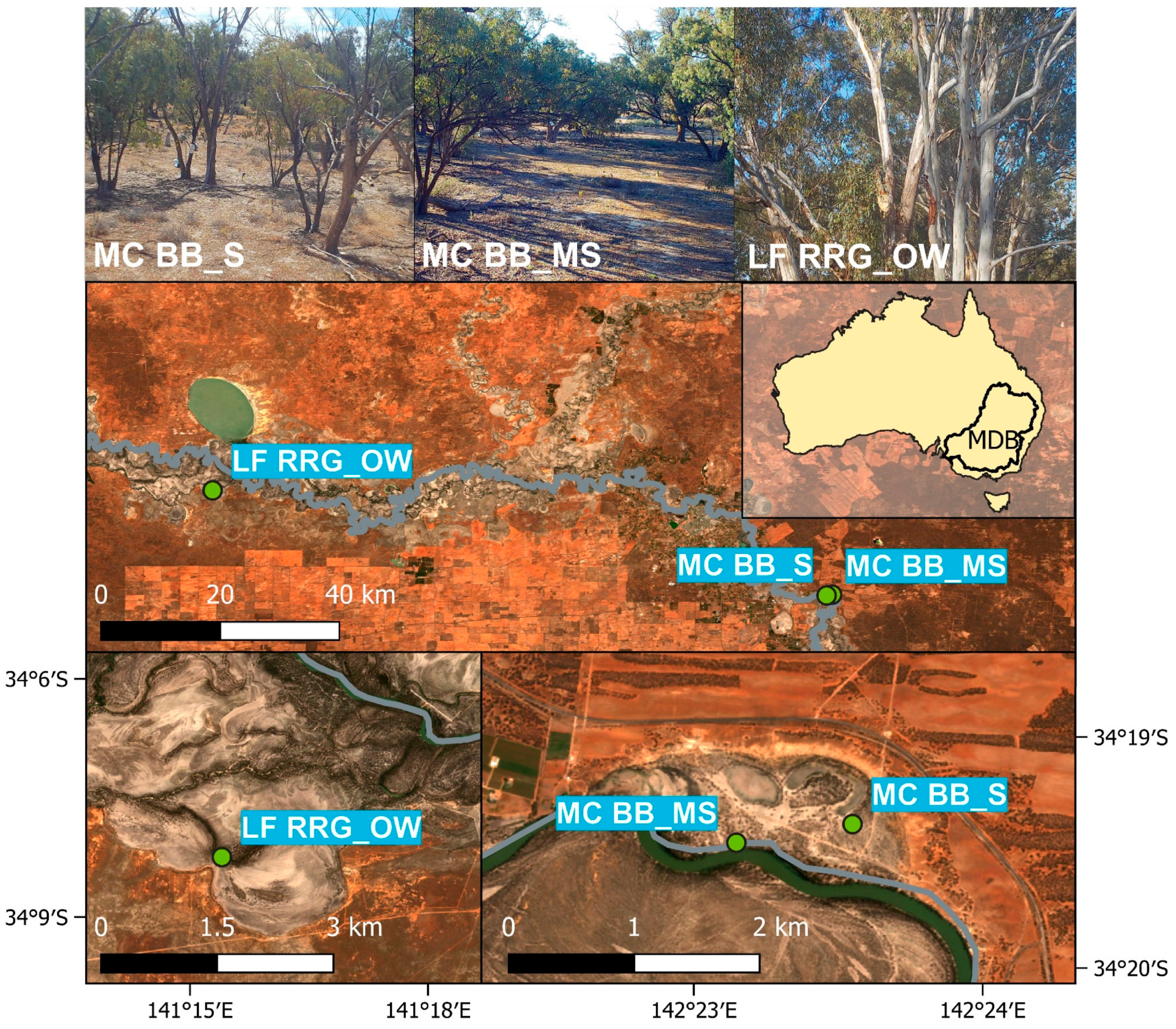
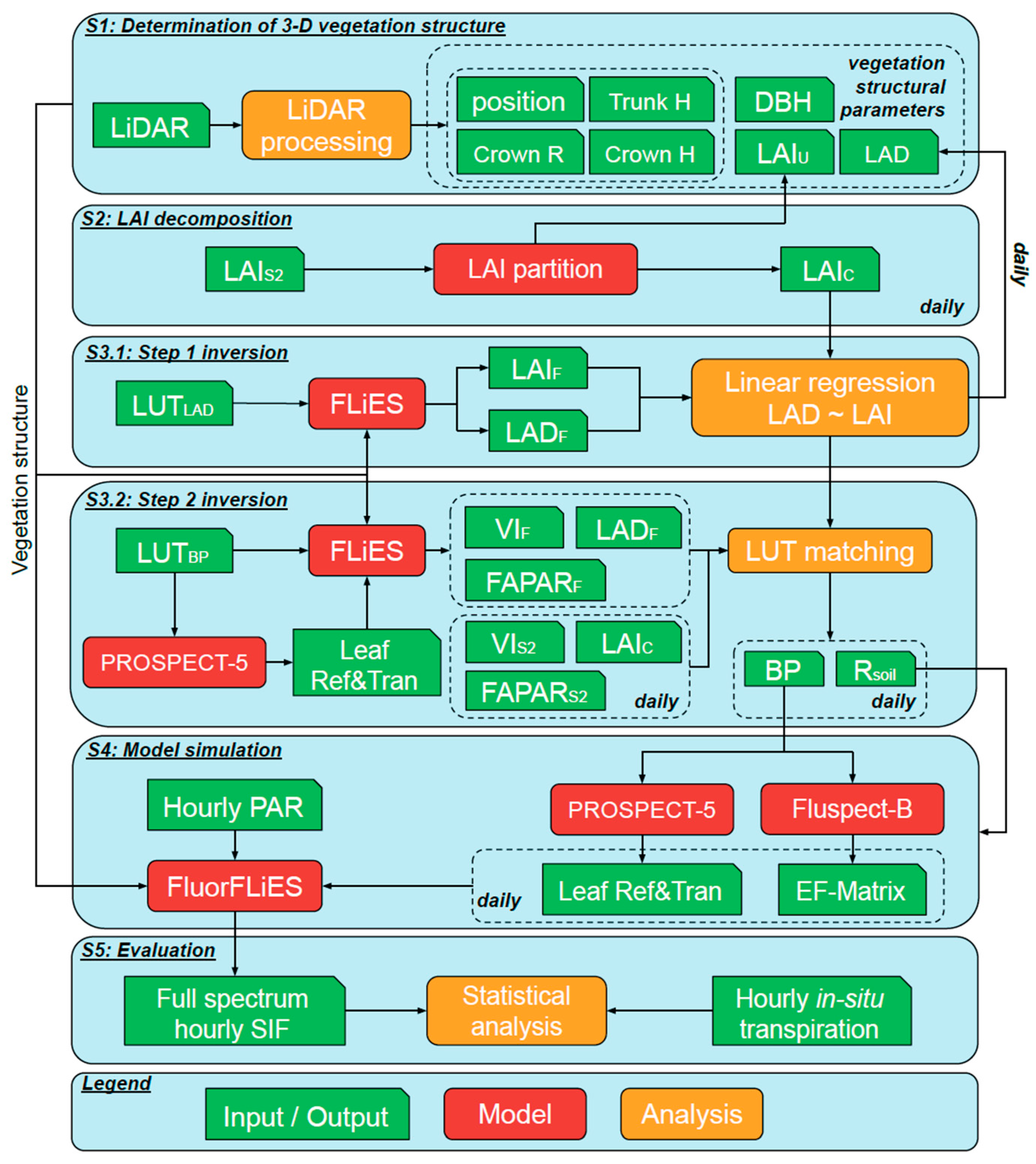
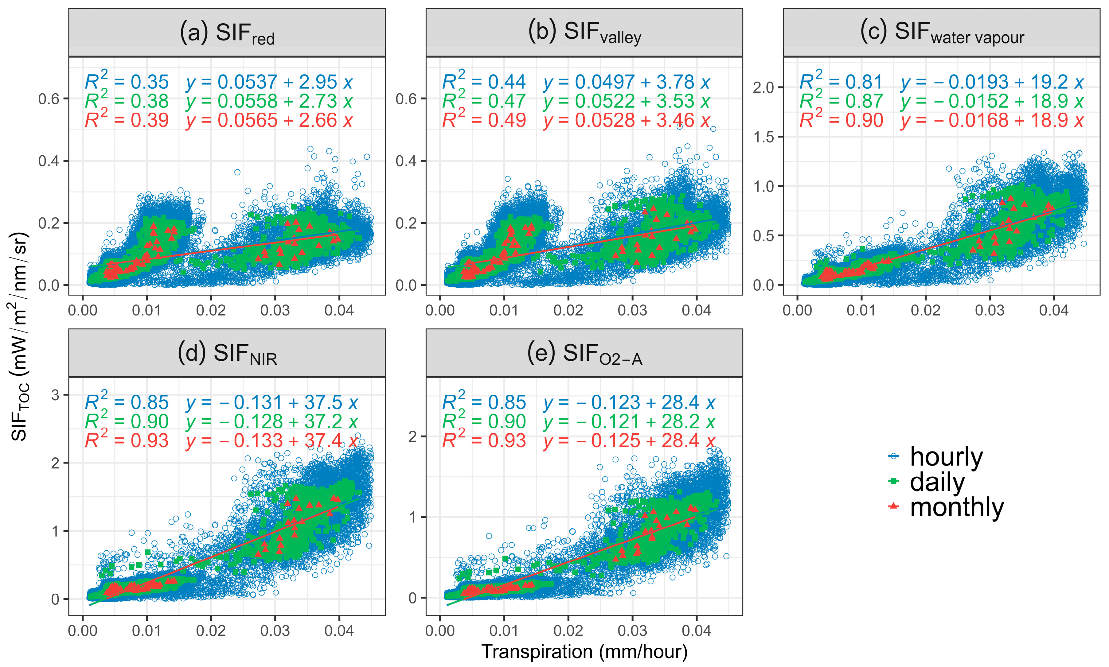

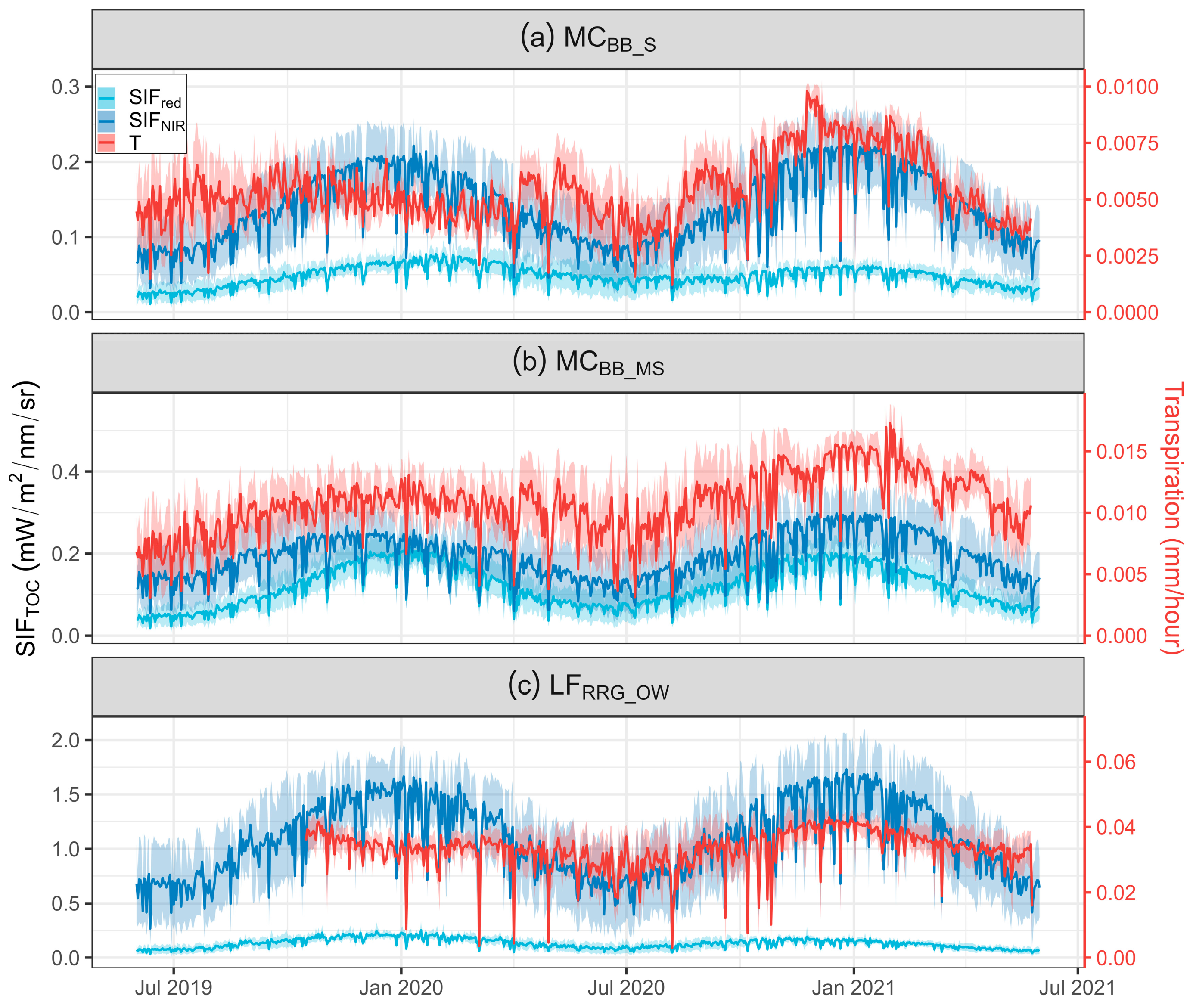
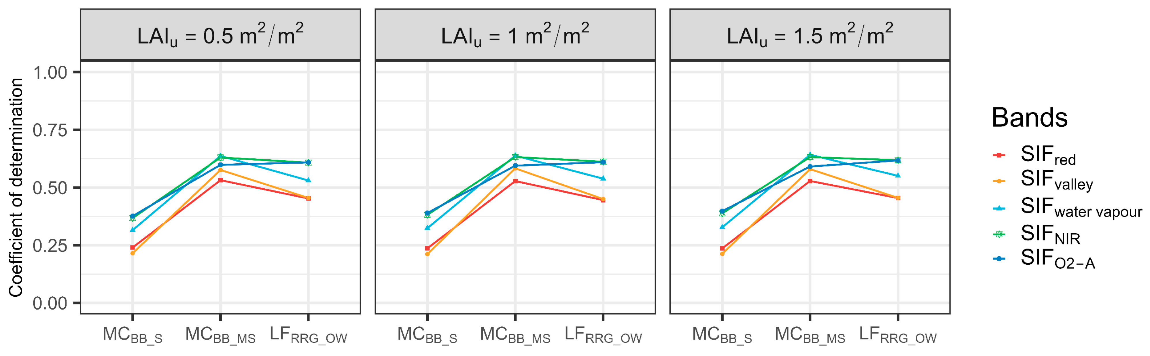

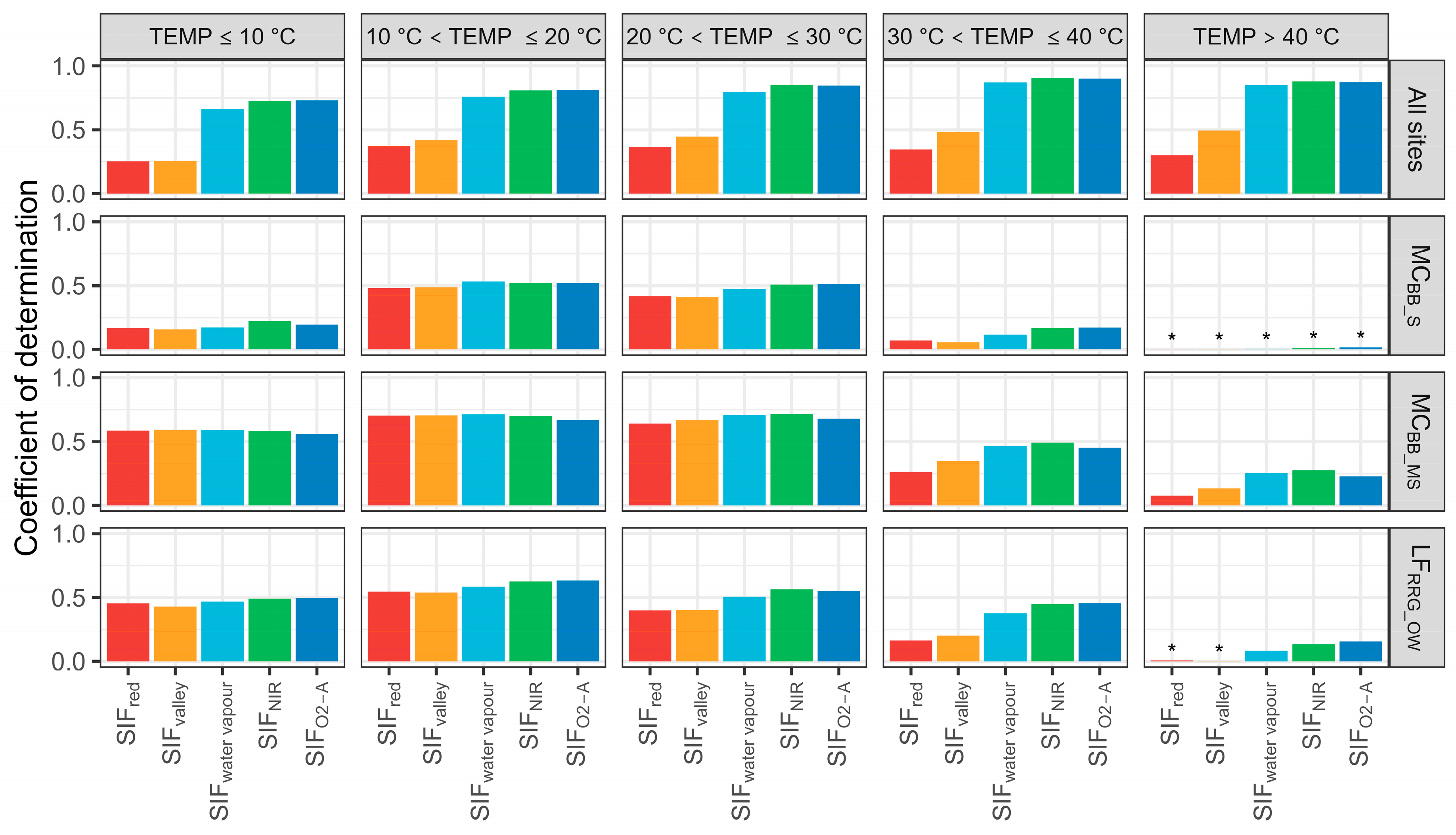
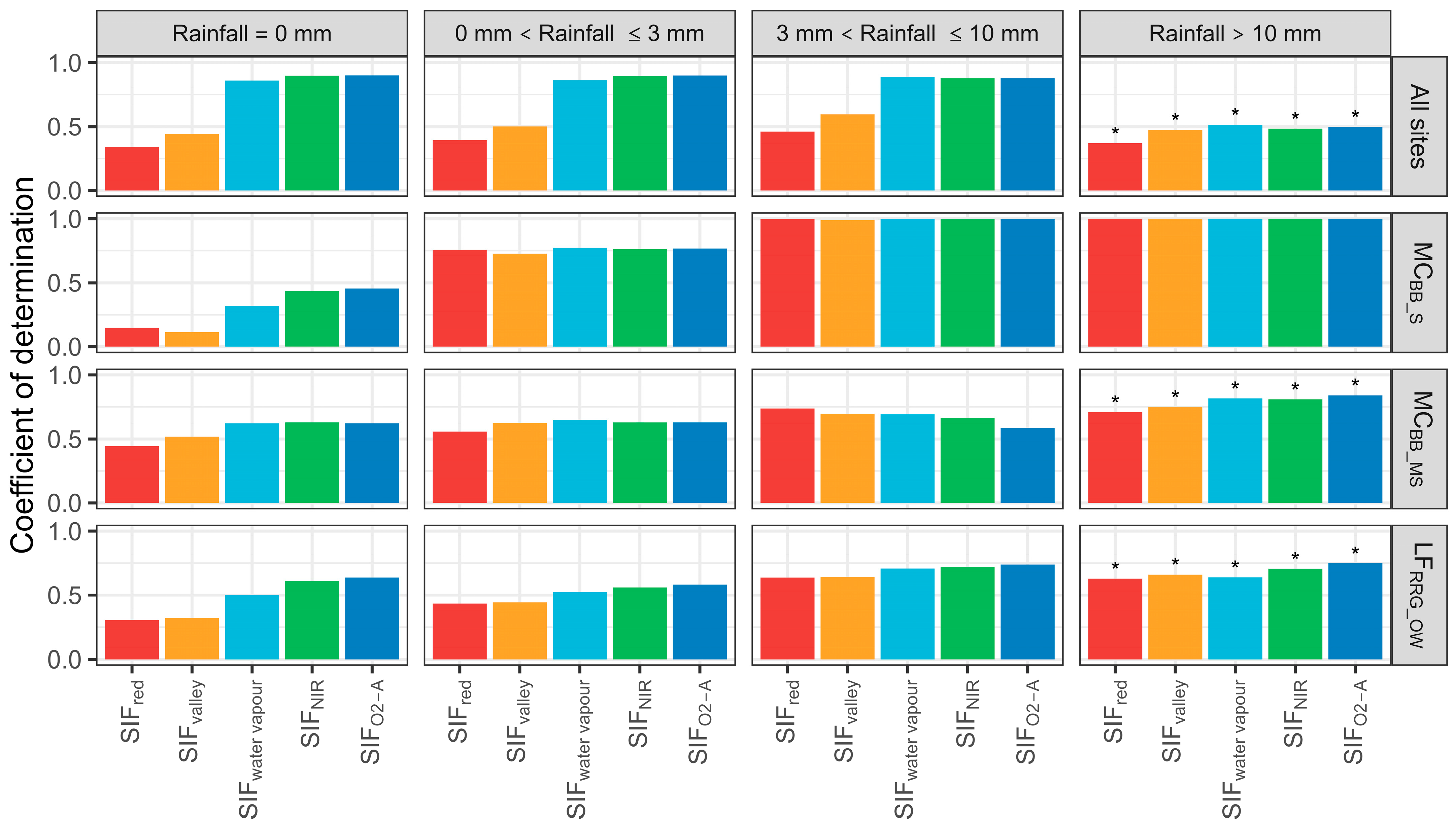
Disclaimer/Publisher’s Note: The statements, opinions and data contained in all publications are solely those of the individual author(s) and contributor(s) and not of MDPI and/or the editor(s). MDPI and/or the editor(s) disclaim responsibility for any injury to people or property resulting from any ideas, methods, instructions or products referred to in the content. |
© 2023 by the authors. Licensee MDPI, Basel, Switzerland. This article is an open access article distributed under the terms and conditions of the Creative Commons Attribution (CC BY) license (https://creativecommons.org/licenses/by/4.0/).