Article

Monitoring of Cotton Boll Opening Rate Based on UAV Multispectral Data

1
Engineering Research Center of Plant Growth Regulator, Ministry of Education, College of Agronomy and Biotechnology, China Agricultural University, Beijing 100193, China
2
Aerospace Information Research Institute, Chinese Academy of Sciences, Beijing 100094, China
3
Shandong Province Agro-Tech Extension and Service Center, Jinan 250100, China
4
Hebei Cottonseed Engineering Technology Research Center, Hejian 062450, China
*
Author to whom correspondence should be addressed.
Remote Sens. 2024, 16(1), 132; https://doi.org/10.3390/rs16010132
Submission received: 27 September 2023 / Revised: 5 December 2023 / Accepted: 18 December 2023 / Published: 28 December 2023

Abstract

:
Defoliation and accelerating ripening are important measures for cotton mechanization, and judging the time of defoliation and accelerating the ripening and harvest of cotton relies heavily on the boll opening rate, making it a crucial factor to consider. The traditional methods of cotton opening rate determination are time-consuming, labor-intensive, destructive, and not suitable for a wide range of applications. In this study, the relationship between the change rate of the vegetation index obtained by the unmanned aerial vehicle multi-spectrum and the ground boll opening rate was established to realize rapid non-destructive testing of the boll opening rate. The normalized difference vegetation index (NDVI) and green normalized difference vegetation index (GNDVI) had good prediction ability for the boll opening rate. NDVI in the training set had an R2 of 0.912 and rRMSE of 15.387%, and the validation set performance had an R2 of 0.929 and rRMSE of 13.414%. GNDVI in the training set had an R2 of 0.901 and rRMSE of 16.318%, and the validation set performance had an R2 of 0.909 and rRMSE of 15.225%. The accuracies of the models based on GNDVI and NDVI were within the acceptable range. In terms of predictive models, random forests achieve the highest accuracy in predictions. Accurately predicting the cotton boll opening rate can support decision-making for harvest and harvest aid spray timing, as well as provide technical support for crop growth monitoring and precision agriculture.

Graphical Abstract

1. Introduction

Cotton is a valuable cash crop and strategic material used in a variety of products. It has a significant correlation with the economies and livelihoods of numerous countries globally. Cotton harvest needs much labor input. In the context of the growing shortage of agricultural labor, mechanization of harvest has become an inevitable trend. Chemical defoliation and ripening are the basis of mechanized cotton harvest. In agricultural practice, the method of spraying the harvest aid is usually adopted to improve the leaf shedding of cotton plants as soon as possible to improve the operation efficiency of mechanical harvesting, reduce the impurity rate of seed cotton, and promote the cracking of bolls [1]. It is very crucial to choose the appropriate time to use the harvest aid in practice, which is difficult to determine [2,3]. Only timely defoliation and ripening can guarantee the effect of defoliation and promote the transfer of the assimilates from the “source” to the “reservoir” to improve cotton yield [4,5]. The accurate monitoring of the boll opening rate enables accurate judgment regarding the time of defoliation and ripening. The most commonly used method to measure the boll opening rate is the five-point sampling method, which means manually measuring or selecting representative plants with uniform growth at different points. However, the results obtained by this method are unrepresentative, non-dynamic, and destructive to in-field cotton plants, which is not conducive to the accurate estimation of the overall boll rate of the cotton field. With the development of agricultural modernization, the traditional methods used to judge the boll opening rate cannot fulfill the requirements of cotton mechanization.
Remote sensing can provide advanced and efficient technical means for the monitoring and diagnosis of crop growth indices and physiological parameters [6,7]. There are three types of remote sensing data available for monitoring the boll opening rate, namely, satellite data, UAV remote sensing, and hand-held spectrometer data. (1) Satellite remote sensing data have been used based on the boll opening rate index, which acquires the most accurate estimation results in both the prediction (R2 = 0.675, RMSE = 7.96%) and validation (R2 = 0.616, RMSE = 2.79%) sets on a regional scale [8]. But interestingly, Zhao et al. showed that the temporal changes in NDVI could explain the differences in agricultural ecosystem cropping systems. This may provide insights for studying the temporal changes in vegetation cover and canopy [9]. (2) Most research on UAV remote sensing focused on predicting the yield after extracting open cotton bolls, and few of them are related to predicting the boll opening rate [10]. (3) Using a handheld Greenseeker red/near-infrared sensor, Owen et al. collected a weekly NDVI of the canopy following mid-bloom. Linear relationships were established between the NDVI of canopy and crop maturity to predict the boll opening rate. The crop maturity was measured as degree-days after planting (DDAP) when the boll opens at the nodes above the white flower (NAWF) = 5 fruiting site [11]. Harris et al. used a GER1500® spectral radiometer to obtain the vegetation reflectance information in the cotton maturity measurement test and built regression models of the NDVI, visible atmospherically resistant index (VARI), and green vegetation index (GVI) on NAWF and the boll opening rate [12]. These studies pointed out that the spectral index had a potential correlation with the crop maturity factor (the boll production rate and NAWF), and aerial images would be of great significance to develop the practical application.
There is also research on extracting cotton bolls from high-resolution images using machine vision to identify the ideal conditions for cotton boll opening [13,14]. Through machine vision, only cotton bolls can be identified, but the information on the boll opening rate cannot be directly obtained. In Ren et al.’s study, the boll opening rate ranged from 0 to 60%. The range of the boll opening rate was not too wide, and the relationship between the boll opening rate and vegetation index was not taken into account after spraying the defoliation ripening agent [8].
While satellite remote sensing data has significant value due to its expansive coverage, the limited spatial resolution poses a challenge in some precision agriculture applications. Forecasting models often cannot provide precise crop yield predictions beyond the county level and fail to capture intricate yield variations at an individual field scale [15,16]. Furthermore, due to the possibility of cloud cover obstructing satellite imagery and its inflexible revisit schedule, timely and comprehensive information on the entire crop growth cycle cannot always be obtained using satellite remote sensing [17]. The hand-held spectrometer method to measure spectral data is time-consuming and laborious. Thus, there is an urgent need for a measurement method that is both effective and relatively accurate. Due to their flexibility and capability of low-altitude flight with centimeter resolution, remote sensing conducted by unmanned aerial vehicles (UAVs) is considered an ideal method for identifying crop phenotypes [18,19,20]. Different types of payloads of unmanned aerial vehicles (UAVs) are based on varying requirements. These types include LiDAR, hyperspectral, multispectral, and RGB cameras. Considering factors such as cost and demand, multispectral and RGB cameras are more widely utilized in practical agricultural applications [21]. Despite the substantial differences in spectral resolution between hyperspectral and multispectral sensors, multispectral cameras equipped with red-edge and near-infrared bands can effectively address a significant portion of crop phenotyping monitoring needs [22]. This includes applications like pest and disease monitoring [23], estimation of crop growth dynamics and yield [24], and inversion of physiological and biochemical traits such as leaf area index and chlorophyll content [25]. Wang et al. achieved favorable results in identifying cotton wilt disease using multispectral UAVs [26], while Chen et al. predicted cotton leaf stripping rates and generated prescription maps based on remote sensing imagery [27].
The existing studies have used the vegetation index to correlate directly with the index to be measured. As we know, the boll opening rate is the ratio of the number of opening bolls to the total number of bolls at a specific time and is an indirect indicator. Therefore, it seems inappropriate to use the vegetation index to directly characterize the cotton boll opening rate. It seems more appropriate to use the opening boll area as a feature to screen the vegetation index, and then characterize the boll opening rate with the rate of change of the vegetation index. Therefore, the target of this study is to establish the relationship between the change rate of vegetation index and the ground boll opening rate in order to realize rapid non-destructive testing of the boll opening rate. To achieve the main target, there are three steps: (1) using a threshold algorithm to extract opening bolls from other components based on an appropriate threshold value, (2) selecting the most relevant vegetation index based on the correlation analysis, and (3) using the change rate of VI to predict boll opening rate and determine the best model.

2. Study Area and Data

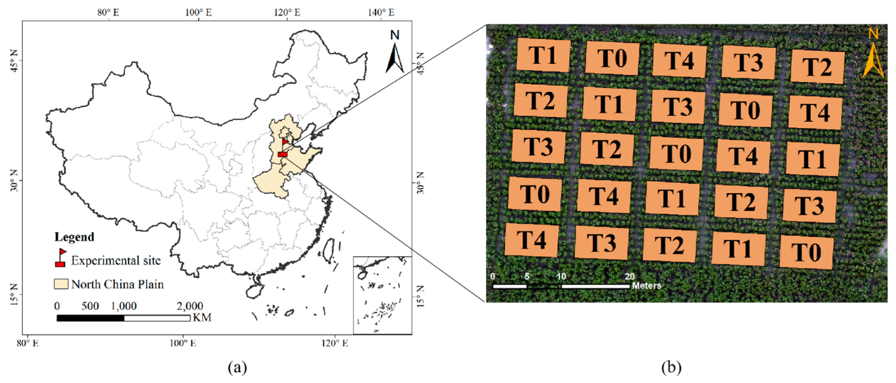
2.1. Study Area and Design of the Experiment

The experiment was conducted in 2021 at the Xi Jiu Ji site, which is located in He Jian (38°23′N, 116°08′E), Hebei Province, China (Figure 1). The site is located in the cotton planting region of the Yellow River basin.
This study adopted a split-plot experiment design. The GuoXin26 variety of cotton was selected in this study, whose planting area was the largest in China. Guoxin 26 is a variety with a growth period of approximately 125 days. It has a columnar plant type with medium-sized leaves. The bolls are elliptical in shape. The plant height is around 98 cm, and the first fruit branch node is located at approximately the 7.2nd node. On average, each plant has about 13.0 fruit branches and produces about 17.2 bolls per plant. It was sowed in April 2021 and harvested in October 2021 with a row spacing of 100 cm and a density of 3.68 × 10⁴ ha−1. The defoliating ripening agent was sprayed on 29 September 2021. The defoliating ripening agent Xinsaili was used to defoliate and ripen the cotton. Xinsaili is the abbreviation for a 50% suspension concentrate of Thiabenzuron and Ethephon (10% Thiabenzuron + 40% Ethephon), with an effective ingredient ratio of 1:4. Before treatment, the growth conditions among the different plots were similar, with an average plant height of 118 cm and a number of fruiting branches of 18. The control group and four defoliating agent treatment groups were established, namely, 0 mL Xinsaili ha−1 (T0), 1500 mL Xinsaili ha−1 (T1), 1500 mL + 1500 mL (i.e., application of a second spray one week after the first application) Xinsaili ha−1 (T2), 3000 mL Xinsaili ha−1 (T3), and 7500 mL Xinsaili ha−1 (T4). Each treatment was replicated five times. Each area of the plot was 63 m2 (9 m × 7 m). The guard row was set as 1 m. For all treatments, the remaining field managements were identical. The utilization of distinct defoliation treatments is primarily intended to shape divergent population conditions during the later growth stage, thereby augmenting the sample dataset and bolstering the model’s robustness.
Hejian’s climate conditions are suitable for cotton cultivation. Daily temperature and precipitation data were recorded by a standard weather station (SPECTRUM WatchDog 2000) located within the field site. From 1 September to 23 October, the average temperature was 17.14 °C; the maximum temperature was 26.64 °C; the minimum temperature was 6.18 °C; and the highest daily rainfall was 36.1 mm.

2.2. Data Collection and Processing

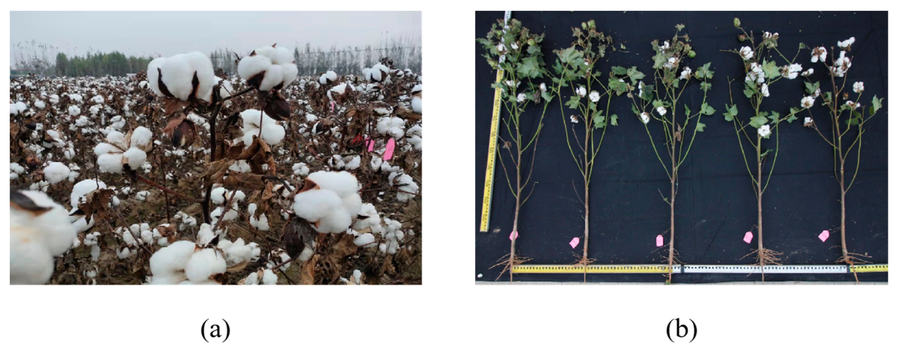
2.2.1. Field Data Collection

The boll opening rate of the cotton plants in the plot was investigated on different dates. Fifteen representative plants were chosen with uniform and consistent growth from five rows in the middle of each plot to investigate the number of opening bolls and total bolls, and opening bolls with a diameter larger than 2 cm were counted. The mean value of 15 plants was taken to represent the boll opening rate of the plot. Refer to Figure 2 for schematic diagrams of the cotton population and individual cotton plants.
The boll opening rate was computed using the following formula:
R B O = N O B N T B × 100 %
RBO refers to the boll opening rate; NOB represents the number of open bolls; and NTB is the total number of bolls on the marked cotton plants within the plot.

2.2.2. Acquisition and Pre-Processing of the UAV Remote Sensing Data

At the same time as the ground sampling, the UAV data was collected synchronously between 11:00 am to 2:00 pm. The DJI (Shenzhen, Guangdong, China) was employed as the UAV platform in this study. It is fitted with a GPS/GNSS satellite positioning system and is capable of bearing up to 1.388 kg of weight and flying for up to 27 min at a time. The payload of the UAV consisted of six 1/2.9-inch CMOS sensors. This set includes one RGB sensor, which captures visible light images, and five monochromatic sensors designed for specific wavelengths: blue (450 nm ± 16 nm), green (560 nm ± 16 nm), red (650 nm ± 16 nm), red edge (730 nm ± 16 nm), and NIR (840 nm ± 26 nm) wavelengths for multi-spectral imaging. Each sensor had an effective pixel count of 2.08 million (see Table 1 for further details). The drone’s flight path was designed using the DJI GsPro 2.0.16 software (DJI, Shenzhen, Guangdong, China), which enabled easy mission planning through various methods such as setting aerial waypoints or importing predefined files. The images were captured at a height of 50 m with 90% overlap and 80% side overlap. The average ground sampling distance is 2.64 cm/pixel. The UAV flew at a speed of 5 m/s. Since the whiteboard was not used for radiometric correction in 2021, the correction coefficient was solved during the same time period in 2022 for radiometric correction of UAV photos in 2021. As shown in Figure 3, the HandHeld2 ground object spectrometer was used to collect hyperspectral curves in six time periods, and the whiteboard photos were taken by UAV at the same time during each collection. The spectral data obtained from the HandHeld2 spectrometer was used for radiometric calibration conducted through the fixed coefficient method. ENVI 5.3 software was used to select each reflection panel image, in turn, to extract the pixel mean value of each calibration panel region in the relative reflectance image. Finally, linear regression between the mean pixel value and the real reflectance was carried out to obtain the radiometric scaling equation. The correction coefficients of the blue band, green band, red band, red edge band, and near-infrared band were, respectively, 4.2309, 2.8996, 2.8994, 2.7181, and 3.1443.
After radiometric calibration, the Pix4D software (Pix4D SA, Lausanne, Switzerland) was used to generate the orthomosaic. The multi-spectral Ag was selected as the template for our model with manually punctured points. By using initialization processing, point cloud, and texture generation, five single-band orthophotos were ultimately generated for each observational stage.

3. Methods

After the acquisition and pre-processing of the UAV data, threshold segmentation was utilized to extract the opening cotton bolls. Afterwards, correlation analysis was conducted to assess the extracted results and twelve selected vegetation indices (VIs) in order to identify the most relevant VIs. The rate of change in the vegetation index was used as the independent variable for predicting cotton boll opening rate. Then, the models were established and evaluated. The method was divided into three parts: (1) opening boll area extraction, (2) selection of vegetation index, and (3) modeling and accuracy evaluation (Figure 4).

3.1. Opening Boll Area Extraction

In ENVI5.3, we select the bolls and non-bolls regions in the RGB image of the cotton field by the tool of ROI (region of interest) and count the range of digital numbers (DNs) on each band of opening bolls and others as shown in Figure 5. The DN refers to the brightness value of a remote-sensing image pixel, recording the dimensionless parameter of the grayscale value of features. In the blue and green bands, the DN values of cotton and other features intersect at different dates, which can cause errors in cotton boll recognition. However, during the growth and development of cotton bolls, in the red band, the minimum value of cotton and the maximum value of others have a minimum difference of 0 and a maximum difference of 17, with no intersection. Therefore, the red band was selected as the threshold segmentation band.

3.2. Selection of VIs

According to the above, the value of the open boll and the background in the red band is quite different, so we selected eight vegetation indices containing the red band from previous related studies and common vegetation indices. Cameras with NIR bands became common, so we selected four additional vegetation indices containing NIR bands to find out whether NIR bands have remarkable performance in cotton boll extraction. The twelve VIs are shown in Table 2. The original multispectral images (Figure 6) were utilized to calculate all VIs, and band math was performed using the open-source software QGIS 3.16. After importing the orthophotos obtained from Pix4D Software into a new QGIS project, the raster calculator function was employed to carry out the band math and produce the initial vegetation index maps. Subsequently, the QGIS 3.22.10 software was used to extract the vegetation index of the region of interest.

3.3. Modeling and Algorithm Accuracy Evaluation

3.3.1. Calculating the Rate of the Vegetation Index Change

In this experiment, we used the rate of change in the vegetation index as the independent variable for predicting the cotton boll opening rate. The rate of change of the vegetation index was computed using the following formula:
VI C = V I o V I s V I o
VIC is the rate of change of the vegetation index; VIo is the vegetation index at the first opening boll of cotton in the plot; and VIS is the vegetation index at different time points under different boll opening rates.

3.3.2. Linear Regression

Linear regression is a kind of regression analysis. Its core idea is to solve the equation between a set of dependent variables and independent variables to obtain the regression function. The error term is usually calculated by the least squares method.
y = β0 + β1x + ε
y represents the dependent variable, x represents the independent variables, β1 stands for partial regression coefficients, and β0 denotes the constant term, while ε is representative of the error term.

3.3.3. Partial Least Squares Regression

PLSR is a classical regression prediction model. It is widely used in spectral regression prediction [28,29,30,40]. The use of PLSR can offer solutions to several problems that are not amenable to ordinary multiple regression. For example, in ordinary multiple linear regression, the multiple correlation of variables can be detrimental to the model. The PLSR approach is effective; in this approach, the data are decomposed and screened in the system to extract the dependent variables, with the greatest power of explanation being chosen as the comprehensive variables to distinguish between the information and noise in the system and better overcome the adverse effects of multiple correlation variables in system modeling. In short, PLSR is a combination of three basic algorithms, namely, PCA, CCA, and multiple linear regression.

3.3.4. Random Forest

Ensemble learning forms the basis of the supervised machine learning algorithm known as RF. The RF model is widely used in remote sensing model prediction [41,42,43]. An RF model comprises multiple decision trees and is considered to be an essential model. The prediction result is obtained by averaging the predictions of all decision trees. This technique reduces variance by training each tree on a subset of data and combining multiple decision trees to determine the final output. In regression problems, the final output is determined by the average of the outputs from all decision trees. Among the popular machine learning algorithms, RF regression is more adept at handling regression problems. Furthermore, this technique is unaffected by the noise present in the training set and produces a robust model.

3.3.5. Evaluation of Model Accuracy

To ensure sufficient training samples and effective validation, the algorithm was trained using a randomly selected 80% of the observed sample data from the field, and the remaining 20% was reserved for validation purposes. To assess the performance of the various models, the coefficient of determination (R2) and relative root mean square error (rRMSE) were employed. Calculation of R2 and rRMSE involved the use of the following equations:
R 2 = 1 1 n y i y ^ i 2 1 n y i y ¯ i 2
r R M S E = 1 n 1 n y i y ^ i 2 y ¯ i
The number of samples can be denoted by n; y ^ i is the predicted value; yi is the actual value; and y ¯ i is the mean of the actual value.

4. Results

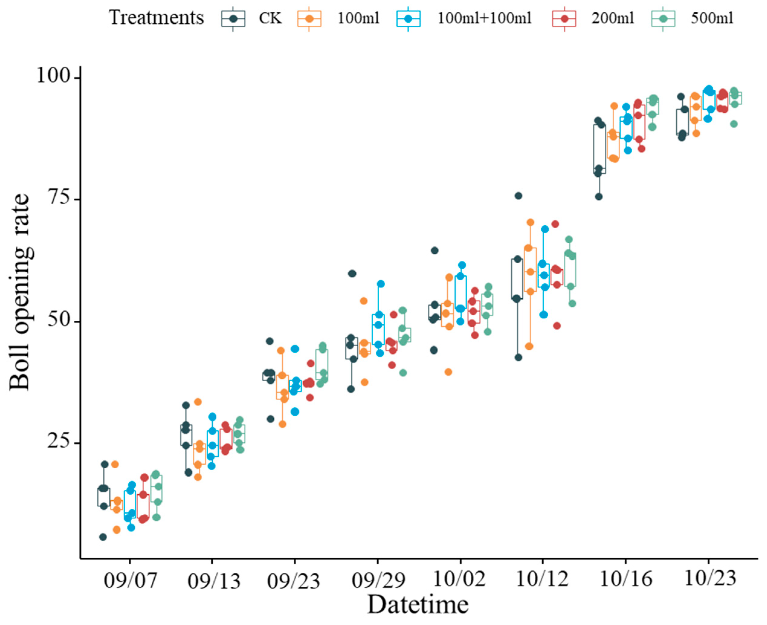
4.1. Variations of the Boll Opening Rate

The information about the date of the survey can be seen in Figure 7, which also shows the descriptive statistics of the boll opening rate by each growth stage and the dynamic of the boll opening rate change with time. Based on Figure 6, it can be observed that there is no obvious difference in boll opening percentage among different defoliant treatments at any time period. However, the trend of boll opening percentage over time was quite interesting. It can be seen that before 12 October, the boll opening percentage showed a slow increase over time. But during the short period of 4 days, from 12 October to 16 October, there was a shocking increase, reaching nearly 80% or more. Through the analysis of meteorological factors, we found that it was likely that the slow increase in the boll opening percentage before 12 October was due to insufficient light and heat conditions caused by cloudy and rainy weather, which delayed the cotton boll opening process. During the period from October 12th to 16th, abundant sunlight accelerated the boll opening process, and previously accumulated unopened cotton bolls were able to open fully, resulting in a rapid increase in the boll opening percentage. Continuous cloudy and rainy weather after defoliation may also be an important reason for the lack of obvious difference in the boll opening percentage among the treatments in the experiment. Across all growth stages, the boll opening rate varied from 5.887 to 97.904%.

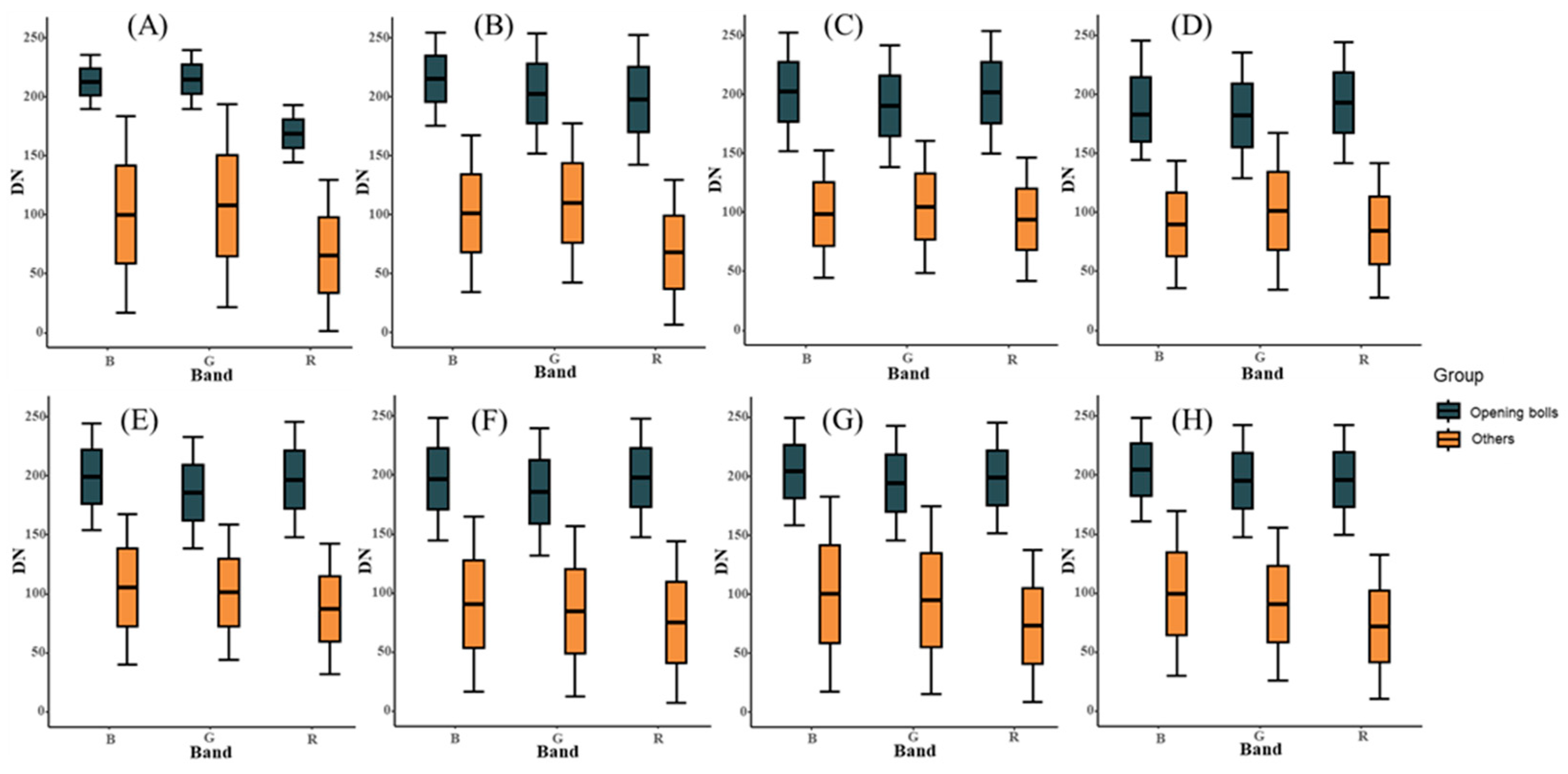
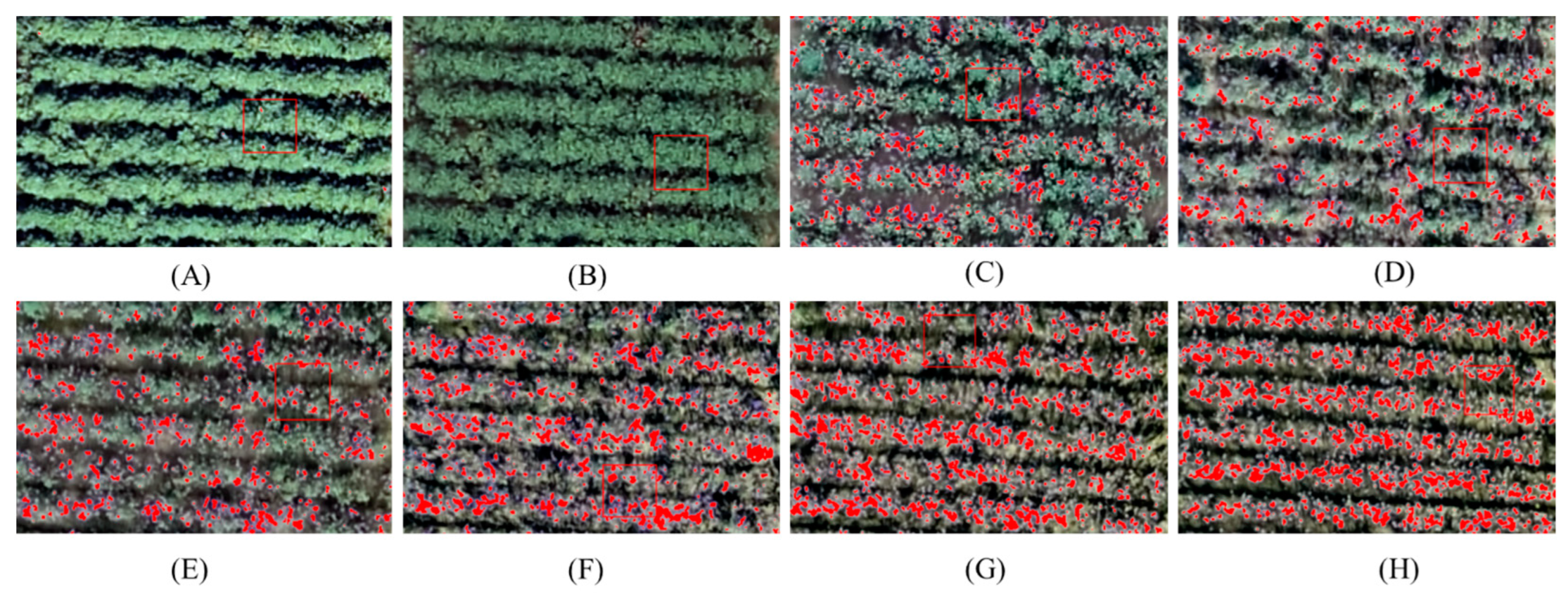
4.2. Extract the Opening Bolls Area Based on the Threshold

The opening bolls’ area is determined by the threshold segmentation method for the red band in the visible image. From Figure 8, we can see the opening bolls’ extraction results in different time periods in a certain cell. The opening boll areas determined by threshold value were compared with the results of visual interpretation. And the accuracy evaluation results are shown in Table 3. The findings indicate that an exceptional level of accuracy was achieved, consistently exceeding 99% across all eight selected days. Additionally, the kappa coefficients surpassed 0.94. That is, the extraction of open cotton bolls demonstrated excellent performance through threshold segmentation.

4.3. Correlation between Vegetation Indices and the Opening Bolls’ Area

Table 4 shows the correlation between the vegetation indices and the opening bolls’ area. The five vegetation indices with the highest correlation coefficient between vegetation indices and the opening bolls’ area were EVI, GNDVI, GRVI, NDVI, and SR and reached a significant level (p < 0.001). All the five vegetation indices included NIR bands, indicating that some plant characteristics reflected by an NIR band, such as canopy photosynthetic capacity and other characteristics, may be related to the change of the boll opening rate. It is worth mentioning that the Spearman correlation analysis was employed in this study, so there is no strict requirement for the normal distribution of data.

4.4. Regression Equations of the Opening Bolls’ Area Estimation Model Based on Each of the Vegetation Indices

We select the five vegetation indices with the strongest correlation in Table 4 for further analysis and calculate the rate of change of these five vegetation indices. Table 5 shows the regression equations of the boll opening rate estimation model based on each of the rate changes of the vegetation indices. The two vegetation indices, namely, NDVI and GNDVI, both showed an R2 greater than 0.900 and an rRMSE smaller than the other indices in both training and validation sets. The linear regression equation of NDVI was y = 101.316x + 15.372. Its training set performance was an R2 of 0.912 and rRMSE of 15.387%, and its validation set performance was an R2 of 0.929 and rRMSE of 13.414%. The linear regression equation of GNDVI was y = 53.333x + 24.562. Its training set performance was an R2 of 0.901 and rRMSE of 16.318%, and its validation set performance was an R2 of 0.909 and rRMSE of 15.225%. NDVI showed the best prediction of the boll opening rate in the training set and validation set.

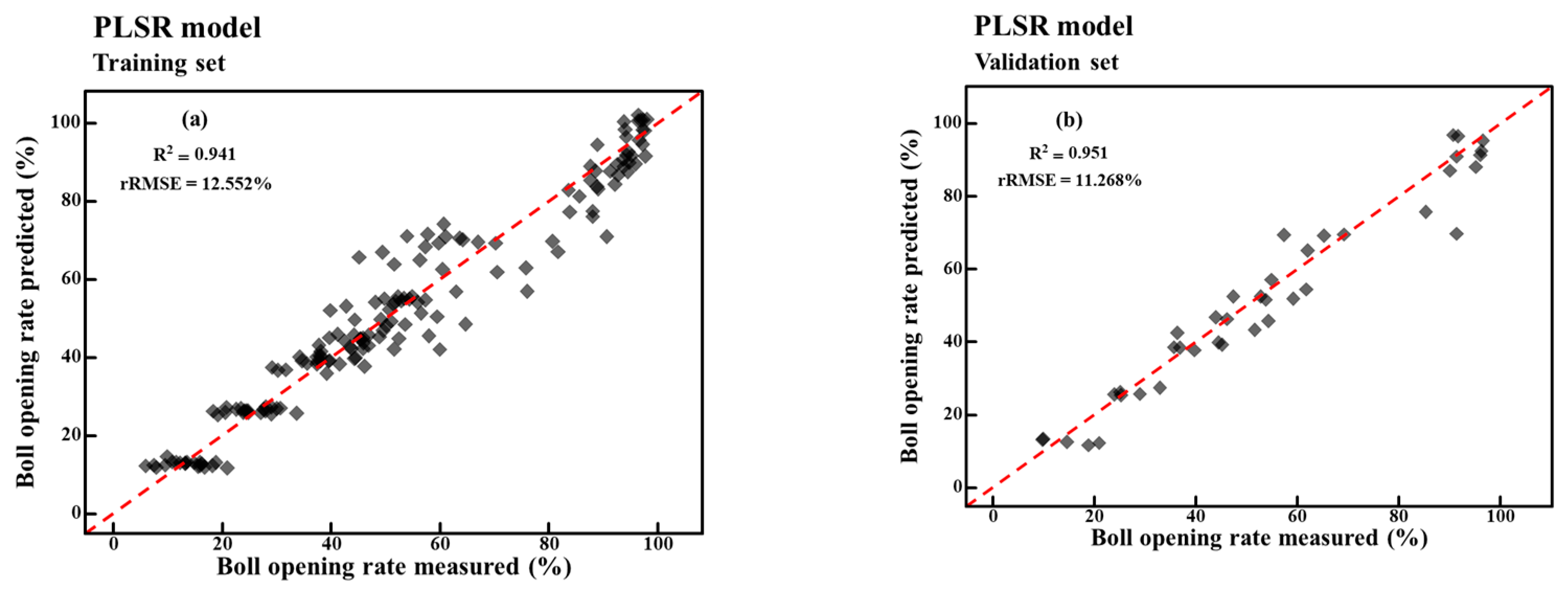
4.5. Boll Opening Rate Model Based on PLSR

The five vegetation indices with the highest correlation coefficient were selected as the independent variables of the model. For the PLSR model, the number of components was selected according to the variance explanation rate. As shown in Table 6, when the component number was three, the variance explanation rate of x was 99.84% and the variance explanation rate of y was 94.12%. In this model, the number of components selected was three.
Figure 9 displays the results of the training set and the validation set based on PLSR. The PLSR model utilizing three components achieved an R2 of above 0.94 and an rRMSE below 13% in both the training and validation sets. Interestingly, the performance on the validation set surpassed that of the training set, indicating the model’s robust generalization ability. Moreover, from Figure 8, it can be observed that the PLSR method exhibited moderate fitting for boll opening rates below 40% in both the training and validation sets. This may be attributed to the complex canopy structure and the model’s limited capacity to fully capture the canopy’s state when boll opening rates are low.

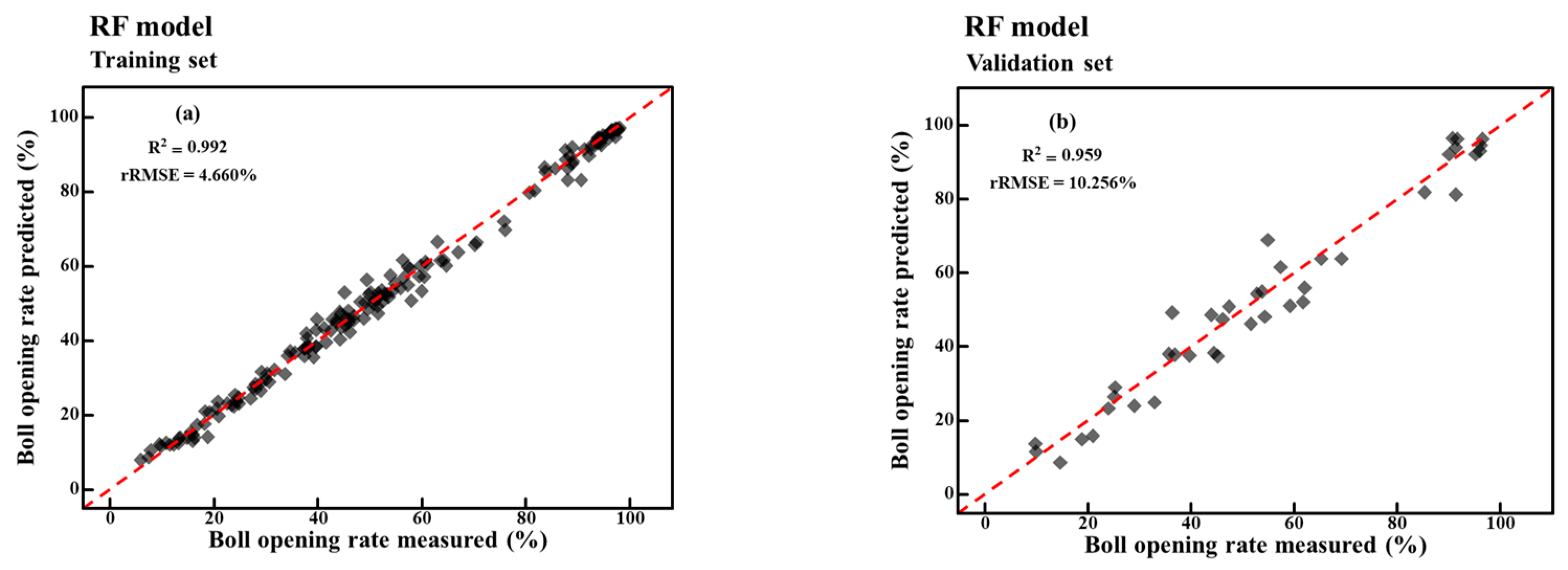
4.6. Boll Opening Rate Model Based on RF

Figure 10 shows the performance of the training and validation sets using RF. In the random forest model, we used rRMSE as an indicator to filter ntree and mtry, and when rRMSE was the smallest, we obtained the values of ntree and mtry. Ntree was 41, and mtry was 5. The RF model performed admirably in predicting the boll opening rate, with R2 values exceeding 0.95 for both the training and validation sets, with a remarkable R2 of 0.992 achieved on the training set. Additionally, the model exhibited rRMSE values below 11% for both datasets. In comparison to the PLSR model, the RF model demonstrated robust predictive capabilities across the entire range of boll opening rates.

5. Discussion

5.1. The Rate of Change of the Vegetation Index Is a More Appropriate Method for the Cotton Boll Opening Rate

Crop spectral properties are influenced by the changes in their light absorption, transmission, and reflection resulting from their physiological characteristics, which reflect the growth status of the crop [44]. The vegetation index is based on this relationship between reflectivity and growth state or characteristics and is calculated by operating on the band. Most vegetation indices are designed for assessing the photosynthetic capacity of plants, which is widely used to describe vegetation dynamics and physiological and biochemical parameters [45,46]. The boll opening rate is the ratio of the number of opening bolls to the total number of bolls at a specific time, which is obviously inconsistent with the original design intent of these vegetation indices. Therefore, it seems inappropriate to use the vegetation index to directly characterize the cotton boll opening rate. However, along with the cotton boll opening, the leaves gradually senesce and the photosynthetic capacity gradually declines. This is because during the boll opening process, the vegetative growth of cotton slows down or even stops and photosynthates are diverted from the leaves to the cotton bolls. As a result, the leaves undergo continual aging, leading to a gradual decline in photosynthetic capacity. This is precisely the rationale behind our intention to employ the change rate of VIs as a means of inferring the boll opening rate.

5.2. The Vegetation Index with a Good Prediction Capability for the Boll Opening Rate

Table 3 shows the relationship between each vegetation index and the opening bolls’ area in the training set and validation set. Then, we select five vegetation indices with strong correlations for further analysis. GNDVI and NDVI showed a good prediction of the boll opening rate in the training set and validation set. Gitelson et al. believe that over a large range of chlorophyll changes (the color of the leaf changed from completely yellow to dark green), GNDVI can accurately estimate pigment concentration [34]. Wang et al. suggested that GNDVI has a wider range of sensitivity to LAI than the red and blue bands [47]. A recent study by Singh et al. showed that GNDVI has a strong correlation with the amount of radiation absorbed for photosynthesis and has a linear relationship with LAI and crop biomass, with the green band being more strongly correlated than the red band. This index is also highly sensitive to plant chlorophyll contents [48]. GNDVI has better sensitivity to the leaf area index and chlorophyll content. As the growth process advances, the leaves undergo aging, change color, and eventually fall off. Fewer leaves mean more cotton bolls have the opportunity to be exposed, and, additionally, the number of opening cotton bolls also increases continuously. Therefore, GNDVI can effectively predict the boll opening rate.
Retrieving the biophysical properties of vegetation canopies with vegetation indices is most commonly achieved using NDVI [49,50,51]. However, if ground biomass is high, NDVI can saturate rapidly. The characteristics of the cotton opening period, which is the period of this study, can effectively avoid this issue. This is because after the cotton enters the boll opening stage, the vegetative growth gradually stops; the cotton gradually enters the complete reproductive growth stage; the leaf color gradually turns yellow from bottom to top; and the leaf area index decreases. Another reason why this experiment was not affected by the saturation effect is the low planting density. Even at the peak growth period of the cotton, the leaf area index remained at only four.

5.3. The Method with Unique Advantages for Predicting the Boll Opening Rate

Among the three methods that we tested, namely, LR, PLSR, and RF, RF had the best predictive ability. The rRMSE of random forest in the training set was 4.660%, and in the validation set it was 10.256%. The RF method, which had the best training performance, was better than the GNDVI in the linear model and the partial least squares methods. RF appears to have unique advantages in predicting crop phenotypes using spectral indices, and previous studies have confirmed this [52].
Although its accuracy was lower than the PLSR and RF methods, the linear model has its own unique characteristics. LR is simple and easy to understand. It can be modeled quickly, especially for data where the relationship to be modeled is not particularly complex and the amount of data is small. The models based on GNDVI and NDVI both demonstrated acceptable levels of accuracy.
Ma et al. utilized correlation coefficients and random forest to screen important variables for lint percentage prediction, including vegetation indices, texture features, and color features. They applied different machine learning algorithms for prediction and obtained a random forest prediction set (R2 = 0.73, RMSE = 19.11%, rRMSE = 46.40%) [53]. Yeom et al. employed high-resolution images captured by unmanned aerial vehicles, extracted random seed points, applied the region growing algorithm and Otsu method to determine the threshold for distinguishing cotton bolls from non-cotton bolls in the images, and established a model to predict yield based on the resultant lint cotton boll area [10]. Ma et al. on the other hand, predicted lint percentage using features such as vegetation indices and color spaces extracted from RGB images, but the prediction accuracy was not high. Moreover, their approach differed from the one proposed in this paper. Yeom’s approach, starting from an “image perspective”, effectively monitored the area of lint cotton bolls, but could not predict the lint percentage. The highlight of this study is the creative utilization of the spatiotemporal variation of lint percentage, inferred by the change rate of vegetation indices, to achieve higher recognition accuracy.

5.4. Limitations of This Study and Suggestions for the Future Boll Opening Rate Estimation

The used method can directly construct the relationship between the vegetation index obtained by UAV and the boll opening rate at a much finer scale and achieve relatively accurate and rapid identification of the boll opening rate. This study only focused on the relationship between the boll opening rate and the change rate of the vegetation index at one density for only one species. The main factors that shape the overall canopy spectral response pattern when evaluating vegetation canopy reflectance are the optical properties of its constituent elements, namely, leaves, stems, and fruits. Under different row spacing, different irrigation volumes, and different density configurations, the distribution of cotton bolls in physical space is distinct. In addition, in the later growth stage, cotton may have three states, namely, normal aging, early maturation, and greedy late maturation, due to the influence of soil, fertilization, or environmental factors. These factors should all be taken into account in future studies. The bolls’ opening follows the order from bottom to top and inside to outside. In the early stage, due to the occlusion of the upper leaves, it is difficult to detect the cotton bolls in the lower layer, and the senescence of the leaves and the overall canopy state of the cotton boll opening rate are not too “coordinated”. Therefore, in the remote sensing image, the vegetation information reflected in the whole canopy due to the change of the boll opening rate in the lower layer is not fully displayed. There may be a segmented linear regression relationship between the change rate of the vegetation index and the boll opening rate, which also needs to be studied in the next step. Yeom et al. employed boll area as a predictive factor for estimating cotton field yield. They observed that an increase in boll area is associated with a corresponding increase in cotton field yield [11]. Additionally, the augmentation of the boll area generally results in an increase in the boll opening rate. Accurately predicting the boll opening rate could serve as a valuable reference for yield forecasting and harvesting decisions. These findings will be further validated in future research endeavors.

6. Conclusions

In this study, we developed a new model for monitoring the boll opening rate of cotton. Based on the correlation results between vegetation indices and the cotton opening boll area, five vegetation indices (EVI, GNDVI, GRVI, NDVI, and SR) with the highest correlation coefficient were selected for further analysis. NDVI exhibited the highest accuracy (R2 = 0.912 and rRMSE = 15.387% in the training set; R2 = 0.929 and rRMSE = 13.414% in the validation set) in predicting the cotton boll opening rate among the change rate of evaluated vegetation indices. The prediction accuracy of GNDVI and NDVI were within the acceptable range. In terms of predictive models, RF achieves the highest accuracy in predictions, with an R2 of 0.992 and rRMSE of 4.660% in the training datasets and an R2 of 0.959 and rRMSE of 10.256% in the validation dataset. We realized rapid non-destructive testing of the boll opening rate by using RF to establish the relationship between the cotton boll opening rate and the change of VIs. The research results demonstrate that the rapid and non-destructive monitoring of the cotton boll opening rate in cotton fields has been achieved by establishing the relationship between the cotton boll opening rate and vegetation index changes using the RF method. Furthermore, the saturation effect of NDVI does not influence the experimental results significantly, due to the gradual leaf senescence in the later growth stage. However, the applicability of this method to cotton populations with significant morphological variations still requires further exploration. Overall, the research findings provide decision support for predicting harvest time and determining the timing of harvest aids application, while also offering technical support for precise agriculture and cotton growth monitoring.

Author Contributions

Conceptualization: Y.W. (Yukun Wang), Q.L., X.D., M.D. and X.T.; Software: Y.W. (Yukun Wang), C.X. and X.D.; Formal analysis: Y.W. (Yukun Wang), Y.W. (Yao Wang) and K.L.; Investigation: Y.W. (Yukun Wang), C.X., Y.W. (Yao Wang), J.G., J.Y. and J.Z.; Resources: H.L., M.D., X.T. and Z.L.; Data curation: Y.W. (Yukun Wang), K.Y., X.D. and M.D.; Writing—original draft: Y.W. (Yukun Wang); Writing—review and editing: Q.L., X.D., M.D. and X.T.; Visualization: Y.W. (Yukun Wang) and C.X.; Project administration: M.Z., M.D., X.T. and Z.L. All authors have read and agreed to the published version of the manuscript.

Funding

This work was jointly funded by the China Agriculture Research System (CARS-15-16) and the Chinese Universities Scientific Fund (2023TC137).

Data Availability Statement

Data are contained within the article.

Acknowledgments

We thank the Guoxin Agricultural Research Association. We are also grateful to Liuwei Xie and Yangyang An for their support in field sampling.

Conflicts of Interest

The authors declare no conflict of interest.

References

  1. Xiao, L.; Liusheng, D.; Zhaohu, L.; Baomin, W.; Zhongpei, H. Physiological bases of chemical accelerated boll maturation and defoliation in cotton. Plant Physiol. J. 2004, 40, 758–762. [Google Scholar]
  2. Gwathmey, C.O.; Bange, M.P.; Brodrick, R. Cotton crop maturity: A compendium of measures and predictors. Field Crops Res. 2016, 191, 41–53. [Google Scholar] [CrossRef]
  3. Snipes, C.E.; Baskin, C.C. Influence of early defoliation on cotton yield, seed quality, and fiber properties. Field Crops Res. 1994, 37, 137–143. [Google Scholar] [CrossRef]
  4. Joel, C.F.; Keith, L.E.; Randy, W.; Alexander, M.S. Timing defoliation applications for maximum yields and optimum quality in cotton containing a fruiting gap. Crop Sci. 2004, 44, 158–164. [Google Scholar]
  5. Zheng, N.; Zhai, W.; Zhang, S.; Zhang, W.; Jiang, G.; Han, R.; Qi, F. Factors affecting cotton maturation and senescence processes and the corre-sponding regulative strategies. Plant Physiol. J. 2014, 50, 1310–1314. [Google Scholar]
  6. Dorigo, W.A.; Zurita-Milla, R.; de Wit, A.J.W.; Brazile, J.; Singh, R.; Schaepman, M.E. A review on reflective remote sensing and data assimilation techniques for enhanced agroecosystem modeling. Int. J. Appl. Earth Obs. 2007, 9, 165–193. [Google Scholar] [CrossRef]
  7. Huang, Y.; Thomson, S.J.; Hoffmann, W.C.; Lan, Y.; Fritz, B.K. Development and prospect of unmanned aerial vehicle technologies for agricultural production management. Int. J. Agric. Biol. Eng. 2013, 6, 1. [Google Scholar]
  8. Ren, Y.; Meng, Y.; Huang, W.; Ye, H.; Han, Y.; Kong, W.; Zhou, X.; Cui, B.; Xing, N.; Guo, A. Novel vegetation indices for cotton boll opening status estimation using sentinel-2 data. Remote Sens. 2020, 12, 1712. [Google Scholar] [CrossRef]
  9. Zhao, H.; Yang, X.; Li, J. MODIS data based NDVI Seasonal dynamics in agro-ecosystems of south bank Hangzhouwan bay. Afr. J. Agric. Res. 2012, 6, 4025–4033. [Google Scholar]
  10. Yeom, J.; Jung, J.; Chang, A.; Maeda, M.; Landivar, J. Automated open cotton boll detection for yield estimation using unmanned aircraft vehicle (UAV) data. Remote Sens. 2019, 10, 1895. [Google Scholar] [CrossRef]
  11. Gwathmey, C.O.; Tyler, D.D.; Yin, X. Prospects for monitoring cotton crop maturity with normalized difference vegetation index. Agron. J. 2010, 102, 1352–1360. [Google Scholar] [CrossRef]
  12. Harris, F.A.; English, P.J.; Sudbrink, D.; Nichols, S.P.; Snipes, C.E.; Wills, G.; Hanks, J. Remote-Sensing Measures of Cotton Maturity—Cutout and Boll Opening. In Proceedings of the Beltwide Cotton Conferences, San Antonio, TX, USA, 5–8 January 2004; pp. 1869–1875. [Google Scholar]
  13. Xu, W.; Yang, W.; Chen, S.; Wu, C.; Chen, P.; Lan, Y. Establishing a model to predict the single boll weight of cotton in northern Xinjiang by using high resolution UAV remote sensing data. Comput. Electron. Agric. 2020, 179, 105762. [Google Scholar] [CrossRef]
  14. Zhu, C.; Ding, J.; Zhang, Z.; Wang, Z. Exploring the potential of UAV hyperspectral image for estimating soil salinity: Effects of optimal band combination algorithm and random forest. Spectrochim. Acta Part A Mol. Biomol. Spectrosc. 2022, 279, 121416. [Google Scholar] [CrossRef] [PubMed]
  15. Maimaitijiang, M.; Sagan, V.; Sidike, P.; Daloye, A.M.; Erkbol, H.; Fritschi, F.B. Crop monitoring using Satellite/UAV data fusion and machine learning. Remote Sens. 2020, 12, 1357. [Google Scholar] [CrossRef]
  16. Xiang, H.; Tian, L. Development of a low-cost agricultural remote sensing system based on an autonomous unmanned aerial vehicle (UAV). Biosyst. Eng. 2011, 108, 174–190. [Google Scholar] [CrossRef]
  17. Homolová, L.; Malenovský, Z.; Clevers, J.G.P.W.; García-Santos, G.; Schaepman, M.E. Review of optical-based remote sensing for plant trait mapping. Ecol. Complex. 2013, 15, 1–16. [Google Scholar] [CrossRef]
  18. Jin, X.; Liu, S.; Baret, F.; Hemerlé, M.; Comar, A. Estimates of plant density of wheat crops at emergence from very low altitude UAV imagery. Remote Sens. Environ. 2017, 198, 105–114. [Google Scholar] [CrossRef]
  19. Xun, L.; Zhang, J.; Yao, F.; Cao, D. Improved identification of cotton cultivated areas by applying instance-based transfer learning on the time series of MODIS NDVI. Catena 2022, 213, 106130. [Google Scholar] [CrossRef]
  20. Feng, A.; Zhou, J.; Vories, E.; Sudduth, K.A. Evaluation of cotton emergence using UAV-based imagery and deep learning. Comput. Electron. Agric. 2020, 177, 105711. [Google Scholar] [CrossRef]
  21. Cuaran, J.; Leon, J. Crop monitoring using unmanned aerial vehicles: A review. Agric. Rev. 2021, 42, 121–132. [Google Scholar] [CrossRef]
  22. Feng, L.; Chen, S.; Zhang, C.; Zhang, Y.; He, Y. A comprehensive review on recent applications of unmanned aerial vehicle remote sensing with various sensors for high-throughput plant phenotyping. Comput. Electron. Agric. 2021, 182, 106033. [Google Scholar] [CrossRef]
  23. Durate, A.; Borralho, N.; Cabral, P.; Caetano, M. Recent advances in forest insect pests and diseases monitoring using uav-based data: A systematic review. Forests 2022, 13, 911. [Google Scholar] [CrossRef]
  24. Fu, Z.; Jiang, J.; Gao, Y.; Krienke, B.; Wang, M.; Zhong, K.; Cao, Q.; Tian, Y.; Zhu, Y.; Cao, W.; et al. Wheat growth monitoring and yield estimation based on multi-rotor unmanned aerial vehicle. Remote Sens. 2020, 12, 508. [Google Scholar] [CrossRef]
  25. Wu, Q.; Zhang, Y.; Zhao, Z.; Xie, M.; Hou, D. Estimation of relative chlorophyll content in spring wheat based on multi-temporal UAV remote sensing. Agronomy 2023, 13, 211. [Google Scholar] [CrossRef]
  26. Wang, C.; Chen, Y.; Xiao, Z.; Zeng, X.; Tang, S.; Lin, F.; Zhang, L.; Meng, X.; Liu, S. Cotton blight identification with ground framed canopy photo-assisted multispectral UAV images. Agronomy 2023, 13, 1222. [Google Scholar] [CrossRef]
  27. Chen, P.; Xu, W.; Zhan, Y.; Yang, W.; Wang, J.; Lan, Y. Evaluation of cotton defoliation rate and establishment of spray prescription map using remote sensing imagery. Remote Sens. 2022, 14, 4206. [Google Scholar] [CrossRef]
  28. Tucker, C.J. Red and photographic infrared linear combinations for monitoring vegetation. Remote Sens. Environ. 1979, 8, 127–150. [Google Scholar] [CrossRef]
  29. Wang, X.; Wang, M.; Wang, S.; Wu, Y. Extraction of vegetation information from visible unmanned aerial vehicle images. Tran. Chin. Society Agric. Eng. 2015, 31, 152–159. [Google Scholar] [CrossRef]
  30. Hunt, E.R.J.; Cavigelli, M.; Daughtry, C.S.T.; McMurtrey, J.I.; Walthall, C.L. Evaluation of digital photography from model aircraft for remote sensing of crop biomass and nitrogen status. Precis. Agric. 2005, 6, 359–378. [Google Scholar] [CrossRef]
  31. Dash, J.; Curran, P.J. Evaluation of the MERIS terrestrial chlorophyll index. Adv. Space Res. 2004, 39, 100–104. [Google Scholar] [CrossRef]
  32. Takebe, M.; Yoneyama, T.; Inada, K.; Murakami, T. Spectral reflectance ratio of rice canopy for estimating crop nitrogen status. Plant Soil. 1990, 122, 295–297. [Google Scholar] [CrossRef]
  33. Kanemasu, E.T. Seasonal canopy reflectance patterns of wheat, sorghum, and soybean. Remote Sens. Environ. 1974, 3, 43–47. [Google Scholar] [CrossRef]
  34. Gitelson, A.A.; Gritz, Y.; Merzlyak, M.N. Relationships between leaf chlorophyll content and spectral reflectance and algorithms for non-destructive chlorophyll assessment in higher plant leaves. J. Plant Physiol. 2003, 160, 271–282. [Google Scholar] [CrossRef] [PubMed]
  35. Woebbecke, D.; Meyer, G.; Mortensen, D. Color indicesfor weed identification under various soil, residue, and lighting conditions. Trans. ASAE 1995, 38, 259–269. [Google Scholar] [CrossRef]
  36. Meyer, G.E.; Hindman, T.; Laksmi, K. Machine vision detection parameters for plant species identification. SPIE Proc. 1999, 14, 3243. [Google Scholar] [CrossRef]
  37. Meyer, G.E.; Neto, J.C. Verification of color vegetation indices for automated crop imaging applications. Comput. Electron. Agric. 2008, 63, 282–293. [Google Scholar] [CrossRef]
  38. Jordan, C.F. Derivation of leaf-area index from quality of light on the forest floor. Ecology 1969, 50, 663–666. [Google Scholar] [CrossRef]
  39. David, R.M.; Rosser, N.J.; Donoghue, D.N.M. Improving above ground biomass estimates of Southern Africa dryland forests by combining Sentinel-1 SAR and Sentinel-2 multispectral imagery. Remote Sens. Environ. 2022, 282, 113232. [Google Scholar] [CrossRef]
  40. Xu, W.; Chen, P.; Zhan, Y.; Chen, S.; Zhang, L.; Lan, Y. Cotton yield estimation model based on machine learning using time series UAV remote sensing data. Int. J. Appl. Earth Obs. 2021, 104, 102511. [Google Scholar] [CrossRef]
  41. Barnes, E.M.; Clarke, T.R.; Richards, S.E.; Colaizzi, P.D.; Haberland, J.; Kostrzewski, M.; Waller, P.; Choi, C.; Riley, E. Coincident Detection of Crop Water Stress, Nitrogen Status and Canopy Density Using Ground-Based Multispectral Data. In Proceedings of the Fifth International Conference on Precision Agriculture, Bloomington, MN, USA, 16–19 July 2000. [Google Scholar]
  42. Ramos, M.A.P.; Osco, P.L.; Furuya, D.E.G.; Gonçalves, W.N.; Santana, D.C.; Teodoro, L.P.R.; Junior, C.A.; Capristo-Silva, G.F.; Li, J.; Baio, F.H.R.; et al. A random forest ranking approach to predict yield in maize with uav-based vegetation spectral indices. Comput. Electron. Agric. 2020, 178, 105791. [Google Scholar] [CrossRef]
  43. Srinet, R.; Nandy, S.; Patel, N.R. Estimating leaf area index and light extinction coefficient using Random Forest regression algorithm in a tropical moist deciduous forest, India. Ecol. Inform. 2019, 52, 94–102. [Google Scholar] [CrossRef]
  44. Teluguntla, P.; Thenkabail, P.S.; Oliphant, A.; Xiong, J.; Gumma, M.K.; Congalton, R.G.; Yadav, K.; Huete, A. A 30-m landsat-derived cropland extent product of Australia and China using random forest machine learning algorithm on Google Earth Engine cloud computing platform. ISPRS J. Photogramm. 2018, 144, 325–340. [Google Scholar] [CrossRef]
  45. Zeng, Y.; Hao, D.; Huete, A.; Dechant, B.; Berry, J.; Chen, J.M.; Joiner, J.; Frankenberg, C.; Bond-Lamberty, B.; Ryu, Y. Optical vegetation indices for monitoring terrestrial ecosystems globally. Nat. Rev. Earth Environ. 2022, 3, 477–493. [Google Scholar] [CrossRef]
  46. Li, F.; Li, D.; Elsayed, S.; Hu, Y.; Schmidhalter, U. Using optimized three-band spectral indices to assess canopy N uptake in corn and wheat. Eur. J. Agron. 2021, 127, 126286. [Google Scholar] [CrossRef]
  47. Wang, F.; Huang, J.; Tang, Y.; Wang, X. New vegetation index and its application in estimating leaf area index of rice. Rice Sci. 2007, 14, 195–203. [Google Scholar] [CrossRef]
  48. Singh, S.; Pandey, P.; Khan, M.S.; Semwal, M. Multi-Temporal High Resolution Unmanned Aerial Vehicle (UAV) Multispectral Imaging for Menthol Mint Crop Monitoring. In Proceedings of the 6th International Conference for Convergence in Technology (I2CT), Maharashtra, India, 2–4 April 2021; Volume 161, p. 20593513. [Google Scholar] [CrossRef]
  49. Jiang, Z.; Huete, A.R.; Chen, J.; Chen, Y.; Li, J.; Yan, G.; Zhang, X. Analysis of NDVI and scaled difference vegetation index retrievals of vegetation fraction. Remote Sens. Environ. 2006, 101, 366–378. [Google Scholar] [CrossRef]
  50. Maestrini, B.; Basso, B. Predicting spatial patterns of within-field crop yield variability. Field Crop. Res. 2018, 219, 106–112. [Google Scholar] [CrossRef]
  51. Tenreiro, T.R.; García-Vila, M.; Gómez, J.A.; Jiménez-Berni, J.A.; Fereres, E. Using NDVI for the assessment of canopy cover in agricultural crops within modelling research. Comput. Electron. Agric. 2021, 182, 106038. [Google Scholar] [CrossRef]
  52. Yang, H.; Yin, H.; Li, F.; Hu, Y.; Yu, K. Machine learning models fed with optimized spectral indices to advance crop nitrogen monitoring. Field Crop. Res. 2023, 293, 108844. [Google Scholar] [CrossRef]
  53. Yiru, M.; Xiangyu, C.; Changping, H.; Tongyu, H.; Xin, L.; Ze, Z. Monitoring defoliation rate and boll-opening rate of machine-harvested cotton based on UAV RGB images. Eur. J. Agron. 2023, 151, 126976. [Google Scholar]
Figure 1. (a) Location of the study area and (b) overview of the experiment site. The five letters in (b), T0 to T4, represent the control group and four defoliating agent treatment groups, which were 0 mL Xinsaili ha−1 (T0), 1500 mL Xinsaili ha−1 (T1), 1500 mL + 1500 mL (i.e., application of a second spray one week after the first application) Xinsaili ha−1 (T2), 3000 mL Xinsaili ha−1 (T3), and 7500 mL Xinsaili ha−1 (T4).
Remotesensing 16 00132 g001
Figure 2. Ground survey of cotton boll opening rate. (a) Image of the cotton group during the harvest season in the year 2021. (b) Diagram of an individual cotton plant in the year 2022.
Remotesensing 16 00132 g002
Figure 3. Remote sensing data collection. (a) An empirical line method was employed for each band (blue, green, red, red edge, and NIR), utilizing three reference reflectance panels (25%, 50%, and 75%). (b) Multispectral data were collected using a DJI P4M.
Remotesensing 16 00132 g003
Figure 4. Overall workflow of the study.
Remotesensing 16 00132 g004
Figure 5. The range of DN values for opening bolls and others in RGB images. (B, G and R) represent the three drone spectral bands mentioned previously: blue (450 nm ± 16 nm), green (560 nm ± 16 nm), and red (650 nm ± 16 nm), respectively. The sub-images represent the range of values for opening bolls and others on September 7th (A), 13th (B), 23rd (C), and 29th (D) and October 2nd (E), 12th (F), 16th (G), and 23rd (H), respectively.
Remotesensing 16 00132 g005
Figure 6. The original multispectral images of all time stages. The sub-images represent the original multispectral images on August 26th (A), September 7th (B), 13th (C), 23rd (D), and 29th (E), and October 2nd (F), 12th (G), 16th (H), and 23rd (I), respectively. Image A marks the date when the first boll on the first fruiting branch of the cotton field began to open, signifying that the cotton entered the boll opening period.
Remotesensing 16 00132 g006
Figure 7. Changes in the boll opening rate over time. September 7th, 13th, 23rd, and 29th and October 2nd, 12th, 16th, and 23rd represent 134, 140, 150, 156, 159, 169, 173, and 180 days after sowing, respectively.
Remotesensing 16 00132 g007
Figure 8. The opening boll extraction results in different time periods in a certain cell. (AH) represent the opening bolls extraction results on September 7th, 13th, 23rd, and 29th and October 2nd, 12th, 16th, and 23rd, respectively.
Remotesensing 16 00132 g008
Figure 9. Results of the training set and the validation set based on PLSR. (a) Prediction results of the training set based on PLSR. (b) Prediction results of the validation set based on PLSR.
Remotesensing 16 00132 g009
Figure 10. Results of the training set and the validation set based on RF. (a) Prediction results of the training set based on RF. (b) Prediction results of the validation set based on RF.
Remotesensing 16 00132 g010
Table 1. Some parameters related to the UAV and sensors.
Aircraft Parameters Camera Parameters
Takeoff weight1487 gFOV62.7°
Diagonal distance350 mmFocal length5.74 mm
Maximum flying altitude6000 mAperturef/2.2
Max ascent speed6 m/sRGB sensor ISO200–800
Max descent speed3 m/sMonochrome sensor gain1–8×
Max speed50 km/hMax image size1600 × 1300
Max flight time27 minPhoto formatJPEG/TIFF
Operating temperature0 °C to 40 °CSupported file systemsFAT32(32 GB); exFAT(>32 GB)
Operating frequency5.72 to 5.85 GHzOperating temperature0 °C to 40 °C
Table 2. The calculation formula of the spectral index.
Vegetation IndexFormulaReferences
Normalized Difference Vegetation Index (NDVI)(NIR − R)/(NIR + R)[28]
Normalized Difference Red Edge (NDRE)(NIR-RE)/(NIR + RE)[29]
Visible-band Difference Vegetation Index (VDVI)(2 × G − R − B)/(2 × G + R + B)[30]
Green Normalized Difference Vegetation Index (GNDVI)(NIR − G)/(NIR + G)[31]
Simple Ratio Index (SR)NIR/R[32]
Green Ratio Vegetation Index (GRVI)NIR/G[33]
Red Green Ratio Index (RGRI)R/G[34]
Difference Vegetation Index (DVI)NIR − R[35]
Excess Green Vegetation Index (EXG)2 × G − R − B[36]
Excess Red Vegetation Index (EXR)1.4 × R − G[37]
Red Edge Soil-Adjusted Vegetation Index (RESAVI)1.5 × (NIR − RE)/(NIR + RE + 0.5)[38]
Enhanced Vegetation Index (EVI)2.5 × (NIR − R)/(NIR + 6 × R − 7.5 × B + 1)[39]
Note: B, G, R, RE, and NIR are the reflectance at the wavelengths of 450, 560, 650, 730, and 840 nm, respectively.
Table 3. Accuracy evaluation results of opening boll extraction.
DateOverall AccuracyKappa Coefficient
7 September99.82%0.945
13 September99.86%0.958
23 September99.16%0.966
29 September99.83%0.991
2 October99.93%0.997
12 October99.98%0.999
16 October99.82%0.994
23 October99.64%0.988
Table 4. Correlation between vegetation indices and opening bolls’ area.
Vegetation Indexr
DVI−0.654 ***
EVI−0.835 ***
EXG−0.815 ***
EXR0.814 ***
GNDVI−0.835 ***
GRVI−0.838 ***
NDRE−0.750 ***
NDVI−0.835 ***
RESAVI−0.810 ***
RGRI0.777 ***
SR−0.838 ***
VDVI−0.794 ***
*** Indicates a strong correlation with a high level of significance, p < 0.001.
Table 5. Results of the training set and the validation set based on the regression equations.
Vegetation IndexModelTraining SetValidation Set
R2rRMSE (%)R2rRMSE (%)
EVIy = 88.580x + 2.3050.81122.4960.83920.165
GNDVIy = 53.333x + 24.5620.90116.3180.90915.225
GRVIy = 97.183x + 3.5810.82521.6660.84119.968
NDVIy = 101.316x + 15.3720.91215.3870.92913.414
SRy = 81.510x − 1.5430.72427.2220.7425.421
Table 6. Fitting results of boll opening percentage trained by PLSR with varying numbers of components.
Data1 Comps2 Comps3 Comps4 Comps5 Comps
X dimension98.5699.2499.84100.98100.00
Y dimension89.7893.5094.1294.1794.26
Disclaimer/Publisher’s Note: The statements, opinions and data contained in all publications are solely those of the individual author(s) and contributor(s) and not of MDPI and/or the editor(s). MDPI and/or the editor(s) disclaim responsibility for any injury to people or property resulting from any ideas, methods, instructions or products referred to in the content.

