Real Aperture Radar Angular Super-Resolution Imaging Using Modified Smoothed L₀ Norm with a Regularization Strategy

Abstract

Restricted by the ill-posed antenna measurement matrix, the conventional smoothed $L_0$ norm algorithm (SL0) fails to enable direct real aperture radar angular super-resolution imaging. This paper proposes a modified smoothed $L_0$ norm (MSL0) algorithm to address this issue. First, as the pseudo-inverse of the ill-posed antenna measurement matrix is required to set the initial values and calculate the gradient projection, a regularization strategy is employed to relax the ill-posedness. Based on the regularization strategy, the proposed MSL0 algorithm can avoid noise amplification when faced with the ill-posed antenna measurement matrix of real aperture radar. Additionally, to prevent local minima problems, we introduce a hard thresholding operator, based on which the proposed MSL0 algorithm can accurately reconstruct sparse targets. Simulations and experimental results verify the performance of the proposed MSL0 algorithm.

1. Introduction

Radar has come to play an increasingly important role in several areas, including autonomous navigation, driverless driving, and ground surveillance [1,2,3,4,5,6,7,8,9,10,11]. Real aperture radar (RAR) can scan an observation area using an antenna to produce two-dimensional range and cross-range imagery. RAR can be used for any imaging geometry, without the need for coherent processing in the cross-range context [12]. Therefore, RAR is of considerable interest for forward-looking imaging, where synthetic aperture radar (SAR) and Doppler beam sharpening (DBS) techniques fail to work [13]. As the range resolution is related to the bandwidth of the transmitted signal and the angular resolution is dependent on the aperture of the antenna, the range resolution typically far outweighs the angular resolution in practical applications, and the problem of low angular resolution is a limiting factor of RAR. Fortunately, echo data along the azimuthal direction can be modeled as a convolution relationship between the target scatterings and the antenna pattern. Deconvolution methods provide potential for improvement in the angular resolution.

Sparse recovery approaches comprise a popular class of deconvolution methods. The sparse recovery problem is an underdetermined linear system, where the unknown vector is assumed to be sparse, meaning that most of its elements are zero. Sparse recovery approaches have been widely used in many fields, such as medical imaging, video processing, source localization, and radar imaging [14,15,16,17]. In radar imaging, SAR, inverse synthetic aperture radar (ISAR), multiple-input multiple-output (MIMO) radar, and ground-penetrating radar have achieved high-resolution imaging with the help of sparse recovery techniques.

For RAR imaging, the target of interest usually only has a few strong scatterers that are sparsely distributed, such as foreign objects on an airport runway. Sparse recovery approaches can be exploited in RAR imaging to enhance the angular resolution [18]. In [19], based on Bayesian theory, the authors assumed the target to have sparse characteristics and employed the Laplace distribution to describe the sparse prior distribution, achieving angular super-resolution imaging. In [20], the authors applied the $L_1$ norm to express the target sparse prior based on the regularization strategy and converted the angular super-resolution problem into an optimization problem. Theoretically, the two types of methods are essentially equivalent, and they aim to address the $L_1$ norm minimization problem. Furthermore, the iterative adaptive approach (IAA) from the sparse spectrum estimation field was applied for angular super-resolution imaging in [21], obtaining similar results to the two above-mentioned sparse approaches.

As mentioned, current sparse recovery algorithms mostly utilize the $L_1$ norm to represent the sparsity of the target. Indeed, mathematically speaking, the $L_0$ norm has stronger sparsity compared to the $L_1$ norm. However, directly solving the $L_0$ norm minimization is an NP-hard problem. Fortunately, in a recent study [22], the authors proposed a smoothed $L_0$ norm (SL0) algorithm, which utilizes a smooth Gaussian function to approximate the $L_0$ norm and then uses the steepest descent and gradient projection to minimize the approximate $L_0$ norm. The SL0 algorithm has higher accuracy and faster convergence speed compared to conventional $L_1$ norm-based sparse recovery algorithms. In radar imaging, we have successfully applied SL0 to SAR [23], ISAR [24], and MIMO radar [25], reducing the computational complexity while improving the imaging quality.

However, little work on the use of the SL0 method for RAR imaging has been reported. After an investigation, we found the existing SL0 algorithm to be unsuitable for RAR imaging. The antenna measurement matrix is seriously ill-posed because of the low-pass characteristic of the antenna in RAR imaging. The SL0 algorithm requires the calculation of the pseudo-inverse of the ill-posed antenna measurement matrix to set the initial value and calculate the gradient projection. For an ill-posed matrix, the error when calculating the pseudo-inverse is too large; as a result, the SL0 algorithm cannot be utilized directly for RAR imaging. Moreover, for the steepest descent, we can easily fall into local minima.

This paper proposes a modified SL0 (MSL0) algorithm. By replacing the ill-posed antenna measurement matrix with the regularization matrix, we avoid the huge error caused by calculating the pseudo-inverse, allowing for the realization of RAR angular super-resolution imaging. In addition, a hard threshold operator is added to prevent local minima and accelerate convergence. Compared with existing angular super-resolution methods, such as the iterative adaptive approach (IAA) [21] and sparse regularization method [20], the proposed method has advantages in terms of super-resolution performance and computational efficiency.

The remainder of this paper is organized as follows. Section 2 introduces the signal model for RAR. In Section 3, the schemes of the proposed MSL0 method are detailed. Section 4 presents the simulation results and a performance comparison between existing methods and the proposed MSL0 method, followed by a discussion in Section 5. In Section 6, experimental data results are presented to further validate the proposed method. Finally, Section 7 presents the conclusions.

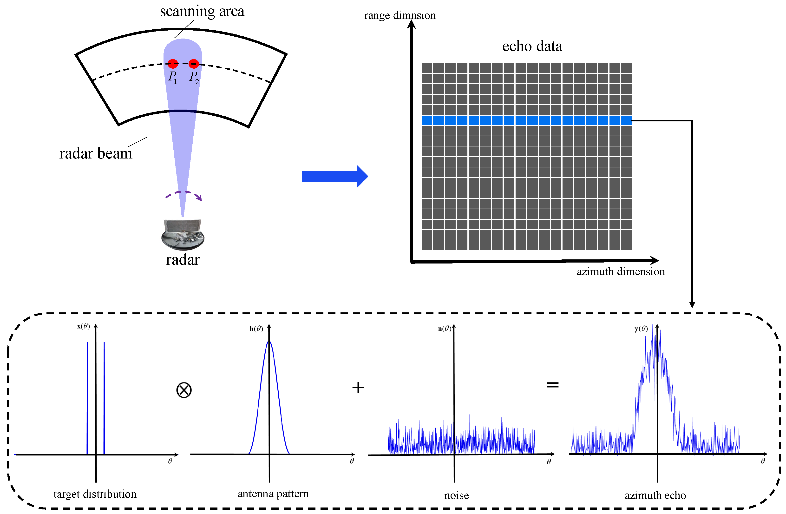
2. Signal Model for Real Aperture Radar Imaging

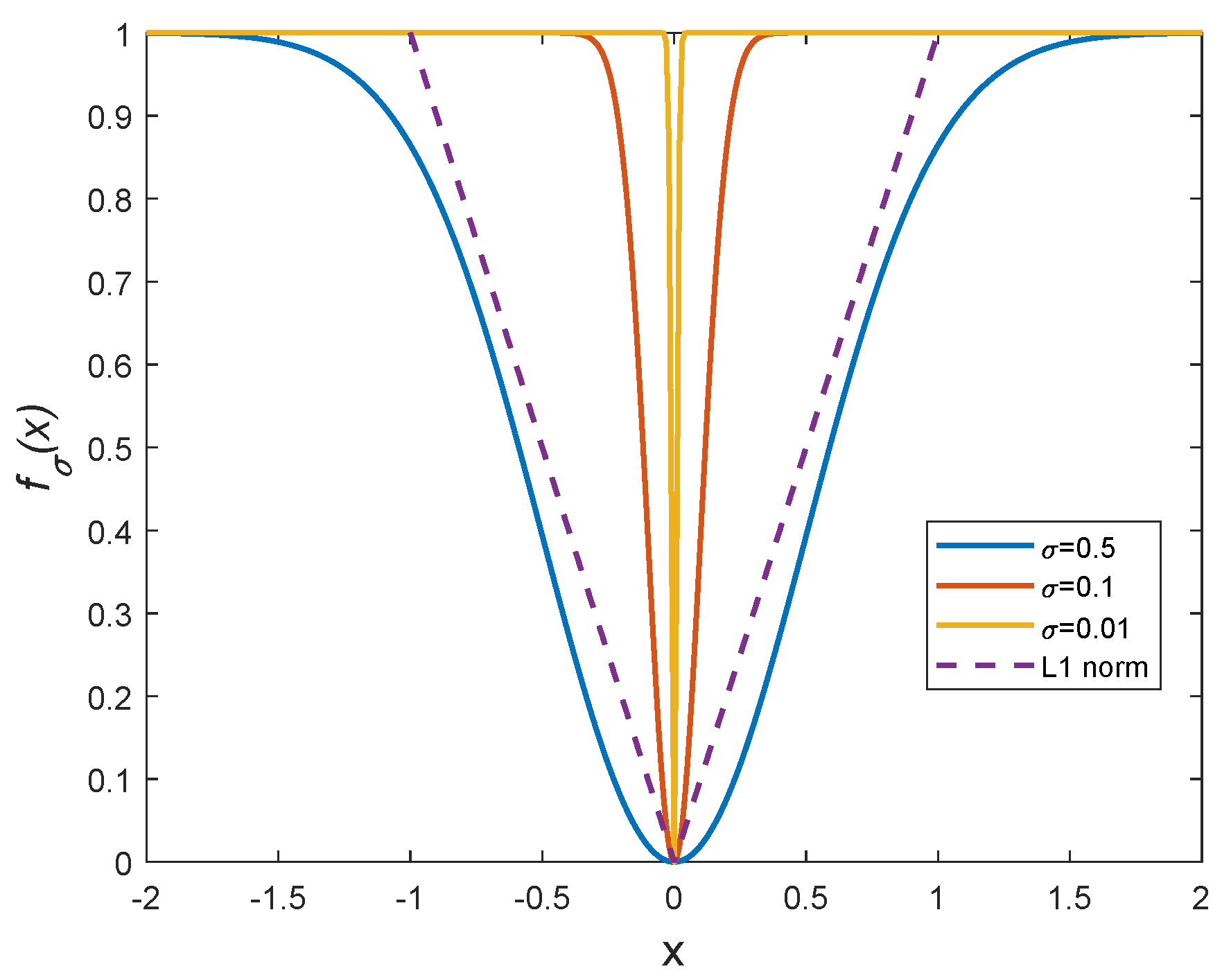
As shown in Figure 1, the RAR acquires echo data through radar beam scanning. The received echo data can achieve high resolution in the range dimension by transmitting a linear frequency modulation (LFM) signal and pulse compression. For the azimuth dimension, according to the sequential process of scanning imaging, the received echo data along the azimuth dimension can be modeled using a one-dimensional convolution model:

$$y\left(\theta \right)=x\left(\theta \right)\otimes h\left(\theta \right)+n\left(\theta \right),$$

(1)

where $\theta$ denotes the azimuth angle, $y\left(\theta \right)$ is the received azimuth echo, $x\left(\theta \right)$ is the target scattering distribution, $h\left(\theta \right)$ is the antenna pattern, $n\left(\theta \right)$ is the noise, and ⊗ is the convolution operation.

After discretization, Equation (1) can be transformed into the following matrix form:

$$\begin{array}{c}\mathit{y}=\mathit{H}\mathit{x}+\mathit{n},\end{array}$$

(2)

where $\mathit{y}={\left[y_{\left({\theta }_1\right)},y_{\left({\theta }_2\right)},\cdots ,y_{\left({\theta }_N\right)}\right]}^T$ is the received azimuth echo vector; $\mathit{x}={\left[x_{\left({\theta }_1\right)},x_{\left({\theta }_2\right)},\cdots ,x_{\left({\theta }_N\right)}\right]}^T$ is the target scattering distribution vector; $\mathit{n}={\left[n_{\left({\theta }_1\right)},n_{\left({\theta }_2\right)},\cdots ,n_{\left({\theta }_N\right)}\right]}^T$ is the noise vector; N represents the number of azimuthal sampling points, which is determined based on the pulse repetition frequency (PRF), scanning scope in the azimuth, and antenna scanning velocity; and H denotes the $N\times N$ antenna measurement matrix composed of the antenna pattern samples shown in Equation (3):

$$\mathit{H}={\left[\begin{array}{ccccc}{h}_{\left({\theta }_0\right)}& \cdots & h_{\left({\theta }_{-l}\right)}& & \\ ⋮& \ddots & & \ddots & \\ h_{\left({\theta }_l\right)}& & \ddots & & h_{\left({\theta }_{-l}\right)}\\ & \ddots & & \ddots & ⋮\\ & & h_{\left({\theta }_l\right)}& \cdots & h_{\left({\theta }_0\right)}\end{array}\right]}_{N\times N},$$

(3)

where $\left[h_{\left({\theta }_{-l}\right)}\cdots h_{\left({\theta }_0\right)}\cdots h_{\left({\theta }_l\right)}\right]$ are the samples of the antenna pattern, and the sampling number is determined according to the PRF, antenna beamwidth, and antenna scanning velocity. As the antenna pattern shown in Figure 2 has low-pass characteristics in the frequency domain, the antenna measurement matrix H is a seriously ill-posed matrix.

Figure 1. Echo acquisition procedure of a real aperture scanning radar.

Figure 1. Echo acquisition procedure of a real aperture scanning radar.

3. Proposed Modified Smoothed ${\mathit{L}}_{\mathbf{0}}$ Norm-Based Method

This section presents a modified smoothed $L_0$ norm (SL0) approach to enhance the angular resolution for sparse targets. Assuming that the target of interest has only a few strong scatterers that are sparsely distributed, most elements in the target scattering vector x are zero. The following optimization problem can be constructed:

$$\widehat{\mathbf{x}}=\underset{\mathbf{x}}{argmin}{∥\mathbf{x}∥}_{0}subjectto∥\mathbf{y}-\mathbf{Hx}∥\le \epsilon ,$$

(4)

where ${∥\mathit{x}∥}_0$ is the penalty term and $\epsilon$ is the noise (or error) energy.

3.1. Main Framework of $L_0$ Norm Minimization

As the $L_0$ norm minimization of a vector is discontinuous, direct minimization is impeded. Therefore, SL0 is employed to approximate this discontinuous function using a suitable continuous one, which can then be optimized with a minimization algorithm for continuous functions. The approximation for the discontinuous function of the $L_0$ norm into a continuous one is as follows:

$$\begin{array}{c}{f}_{\sigma }\left(x_i\right)\triangleq 1-exp(-\frac{{x_i}^2}{2{\sigma }^2}).\end{array}$$

(5)

The accuracy of this approximation is controlled by the parameter $\sigma$. When $\sigma$ is large, the approximation is poor, whereas when $\sigma$ is very small, the approximation tends to be accurate. A small $\sigma$ leads to stronger sparsity compared to the $L_1$ norm, as illustrated in Figure 3. Therefore, we provide a better approximation to the $L_0$ norm of the vector x as follows:

$$\begin{array}{c}{\displaystyle \sum _{i=1}^N}\underset{\sigma \to 0}{lim}{f}_{\sigma }\left(x_i\right)={∥\mathit{x}∥}_0,\end{array}$$

(6)

$$\begin{array}{c}{F}_{\sigma }\left(x\right)={\displaystyle \sum _{i=1}^N}{f}_{\sigma }\left(x_i\right).\end{array}$$

(7)

To minimize the $L_0$ norm, $F_{\sigma }\left(\mathit{x}\right)$ should be minimized. However, a small $\sigma$ value results in a non-smooth approximation containing many local maxima. To avoid these local maxima, a decreasing sequence for the value of $\sigma$ is employed. Therefore, the $L_0$ norm optimization problem based on $F_{\sigma }\left(\mathit{x}\right)$ function minimization can be described as

$$\widehat{\mathbf{x}}=\underset{\sigma \to 0}{lim}\underset{\mathbf{x}}{argmin}{F}_{\sigma }\left(\mathbf{x}\right)subjectto∥\mathbf{y}-\mathbf{Hx}∥\le \epsilon .$$

(8)

3.2. Traditional SL0 Algorithm

In this subsection, a brief review of the traditional SL0 algorithm is given, which mainly includes two parts: the initialization of the traditional SL0 algorithm and the main loop of the traditional SL0 algorithm.

3.2.1. Initialization of Traditional SL0 Algorithm

The core of initialization is to choose a proper initial value for the vector x. In the conventional SL0 algorithm [22], a choice for this initial value ${\widehat{\mathit{x}}}_0$ is given using the pseudo-inverse of H: ${\widehat{\mathit{x}}}_0={\mathit{H}}^T{\left(\mathit{H}{\mathit{H}}^T\right)}^{-1}\mathit{y}$. In addition, a suitable decreasing sequence for $\sigma$ needs to be provided for the algorithm. In [22], the initial value for the $\sigma$ sequence was set as $\sigma =2max\left|{\widehat{\mathit{x}}}_0\right|$. Then, the value of $\sigma$ decreased according to a decreasing coefficient $\rho (0<\rho <1)$.

3.2.2. Main Loop of Traditional SL0 Algorithm

For each value of $\sigma$, a fixed number of steps L in the steepest ascent approach is used to minimize $F_{\sigma }\left(\mathit{x}\right)$. In each steepest ascent iteration, the solution moves in the desired direction, as follows:

$$\begin{array}{c}\widehat{\mathit{x}}\leftarrow \widehat{\mathit{x}}-u_k\nabla F_{\sigma }\left(\mathit{x}\right),\end{array}$$

(9)

where $u_k=u{\sigma }^2$, and u represents a small positive that determines the step size of the algorithm. Furthermore, $\nabla F_{\sigma }\left(\mathbf{x}\right)$ can be expressed as follows:

$$\nabla F_{\sigma }\left(\mathit{x}\right)=\left[-\frac{x_1}{{\sigma }^2}exp(-\frac{x_1}{2{\sigma }^2}),\cdots ,-\frac{x_N}{{\sigma }^2}exp(-\frac{x_N}{2{\sigma }^2})\right].$$

(10)

After the steepest ascent, the following is the projection of the solution into the feasible region, which is performed as:

$$\begin{array}{c}\widehat{\mathit{x}}\leftarrow \widehat{\mathit{x}}-{\mathit{H}}^T{\left(\mathit{H}{\mathit{H}}^T\right)}^{-1}(\mathit{H}\widehat{\mathit{x}}-\mathit{y}).\end{array}$$

(11)

The main loop continues until a minimum value of ${\sigma }_J$ is reached. The SL0 algorithm is summarized in Algorithm 1.

3.3. Proposed MSL0 Algorithm

In the conventional SL0 algorithm, the initial value, descending sequence initial value, and gradient projection all involve the pseudo-inverse of the antenna measurement matrix H. However, as H is a seriously ill-posed matrix, calculating its pseudo-inverse yields a significant error, which has two consequences. Firstly, the final imaging result deviates from the true value because of incorrect initial value setting and gradient projection. As a result, the SL0 method cannot be directly applied for RAR angular super-resolution. Secondly, the descending sequence initial value may become abnormally large, increasing the number of outer loops of the SL0 method and thereby adding to the computational burden.

Algorithm 1 Conventional SL0 algorithm

Initialization:

1. $SetL>0,u>0,0<\rho <1,{\sigma }_J>0$

(e.g., $L=5,u=2,\rho =0.5,{\sigma }_J=0.01)$

2. $Set{\widehat{\mathit{x}}}_0={\mathit{H}}^T{\left(\mathit{H}{\mathit{H}}^T\right)}^{-1}\mathit{y},{\sigma }_0=2max\left|{\widehat{\mathit{x}}}_0\right|;$,

Mainloop:

$Forj=1,\cdots ,J$

$set\widehat{\mathit{x}}={\widehat{\mathit{x}}}_{j-1},\sigma ={\sigma }_{j-1};$

$forl=1,2,3,\cdots ,L$

$\widehat{\mathit{x}}\leftarrow \widehat{\mathit{x}}-u_k\nabla F_{\sigma }\left(\mathit{x}\right);$

$\widehat{\mathit{x}}\leftarrow \widehat{\mathit{x}}-{\mathit{H}}^T{\left(\mathit{H}{\mathit{H}}^T\right)}^{-1}(\mathit{H}\widehat{\mathit{x}}-y);$

$end$

${\sigma }_j=\rho {\sigma }_{j-1},{\widehat{\mathit{x}}}_j=\widehat{\mathit{x}};$

$j=j+1;$

end

Output: $\widehat{\mathit{x}}={\widehat{\mathit{x}}}_J$

3.3.1. Regularization Strategy for Antenna Measurement Matrix

To address the above problems, we introduce a regularization strategy to repair the antenna measurement matrix. The singular value decomposition (SVD) transformation is performed on the antenna measurement matrix as follows:

$$\mathit{H}=\mathit{UDV}=\sum _{i=1}^N{u}_i{d}_i{v_i}^T,$$

(12)

where $\mathit{U}=({\mathit{u}}_1,{\mathit{u}}_2,\dots ,{\mathit{u}}_N)$ and $\mathit{V}=({\mathit{v}}_1,{\mathit{v}}_2,\dots ,{\mathit{v}}_N)$ are unitary matrices of size $N\times N$, and $\mathit{D}=\mathrm{diag}(d_1,d_2\cdots ,d_N)$, $d_{\mathrm{i}}$ is composed of the singular values of H, which satisfies $d_1>d_2>d_i>\dots >d_N$.

The pseudo-inverse of the antenna measurement matrix can be expressed using the singular value decomposition transformation:

$${\mathit{H}}^{†}={\mathit{H}}^T{\left(\mathit{H}{\mathit{H}}^T\right)}^{-1}\mathit{y}=\sum _{i=1}^N{\mathit{v}}_i{{\mathit{v}}_i}^T\mathit{x}+\sum _{i=1}^N{\mathit{v}}_i{{\mathit{u}}_i}^T\frac{\mathit{n}}{d_i}.$$

(13)

Because of the serious ill-posedness of H, inevitably, many small singular values are close to zero. The inversion of small singular values causes noise to be amplified in $\frac{\mathbf{n}}{d_i}$, thus introducing significant errors. To alleviate the influence of the inversion of small singular values, a regularization strategy is adopted to repair the antenna measurement matrix. As a result, the pseudo-inverse is replaced with the following equation:

$${\mathit{H}}_R^{†}={\mathit{H}}^T{(\mathit{H}{\mathit{H}}^T+\lambda \mathit{I})}^{-1}\mathit{y}=\sum _{i=1}^N\frac{{d_i}^2}{{d_i}^2+\lambda }{\mathit{v}}_i{{\mathit{v}}_i}^T\mathit{x}+\sum _{i=1}^N{\mathit{v}}_i{{\mathit{u}}_i}^T\frac{d_i\mathit{n}}{{d_i}^2+\lambda },$$

(14)

where $\lambda$ is the regularization parameter.

From the above equation, after the regularization process, we obtain $\frac{d_i\mathbf{n}}{{d_i}^2+\lambda }=\frac{\mathbf{n}}{d_i+\frac{\lambda }{d_i}}$. With the addition of $\frac{\lambda }{d_i}$ in the denominator, the noise amplification caused by the inversion of small singular values is avoided. By replacing ${\mathit{H}}^{†}$ with ${\mathit{H}}_R^{†}$, we can avoid introducing errors, thereby obtaining a stable azimuth super-resolution imaging result.

3.3.2. Hard Threshold Operator in the Iterative Procedure

The next modification is to prevent falling into local minima. As the search path assumes a sawtooth shape in the process of searching for the optimal value via steepest descent, a hard threshold operation, which is an element-wise operator with low computational complexity, is utilized. The hard threshold operator is defined as

$$\begin{array}{c}hard(\mathit{w},\delta )=\left\{\begin{array}{c}\mathit{w},\left|w\right|\ge \delta \hfill \\ 0,\left|\mathit{w}\right|<\delta \hfill \end{array}\right.,\end{array}$$

(15)

where w is the variable and $\delta$ is the threshold.

By employing the hard threshold operator, any element of $\widehat{x}$ that falls below the set threshold $\delta$ is set to zero. By using a hard threshold operator, falling into local minima is prevented. Furthermore, the problem-solving speed increases with each step. The threshold $\delta$ is an important parameter, and a suggested way to select $\delta$ is to set it as 0.01$max\left|{\widehat{\mathit{x}}}_0\right|$. The MSL0 algorithm for RAR imaging is summarized in Algorithm 2.

Algorithm 2 The MSL0 algorithm

Initialization:

1. $SetL>0,u>0,0<\rho <1,{\sigma }_J>0,\lambda >0$

(e.g., $L=5,u=2,\rho =0.5,{\sigma }_J=0.01,\lambda =2)$

2. $Set{\widehat{\mathit{x}}}_0={\mathit{H}}^T{({\mathit{H}}^T\mathit{H}+\lambda \mathit{I})}^{-1}\mathit{y},{\sigma }_0=2max\left|{\widehat{\mathit{x}}}_0\right|,$

$\delta =0.01max\left|{\widehat{\mathit{x}}}_0\right|;$

Mainloop:

$Forj=1,\cdots ,J$

$set\widehat{\mathit{x}}={\widehat{\mathit{x}}}_{j-1},\sigma ={\sigma }_{j-1};$

$forl=1,2,3,\cdots ,L$

$\widehat{\mathit{x}}\leftarrow \widehat{\mathit{x}}-u_k\nabla F_{\sigma }\left(\mathit{x}\right);$

$\widehat{\mathit{x}}\leftarrow \widehat{\mathit{x}}-{\mathit{H}}^T{({\mathit{H}}^T\mathit{H}+\lambda \mathit{I})}^{-1}(\mathit{H}\widehat{\mathit{x}}-\mathit{y});$

$\widehat{\mathit{x}}\leftarrow hard(\widehat{\mathit{x}},\delta );$

$end$

${\sigma }_j=\rho {\sigma }_{j-1},{\widehat{\mathit{x}}}_j=\widehat{\mathit{x}};$

$j=j+1;$

end

Output: $\widehat{\mathit{x}}={\widehat{\mathit{x}}}_J$

3.3.3. Complexity Analysis of the Proposed Algorithm

During initialization, we can calculate the matrix ${\mathit{H}}^T{({\mathit{H}}^T\mathit{H}+\lambda \mathit{I})}^{-1}$ and the target scattering coefficient ${\widehat{\mathit{x}}}_0={\mathit{H}}^T{({\mathit{H}}^T\mathit{H}+\lambda \mathit{I})}^{-1}\mathit{y}$ and set the parameters in advance. Therefore, we mainly analyze the complexity within the main loop. Suppose the number of outer loops is J and the number of inner loops is L.

For inner loops, computing $\widehat{\mathit{x}}\leftarrow \widehat{\mathit{x}}-u_k\nabla F_{\sigma }\left(\mathit{x}\right)$ involves an element-wise calculation, the complexity of which is $O\left(N\right)$; computing $\widehat{\mathit{x}}\leftarrow \widehat{\mathit{x}}-{\mathit{H}}^T{({\mathit{H}}^T\mathit{H}+\lambda \mathit{I})}^{-1}(\mathit{H}\widehat{\mathit{x}}-\mathit{y})$ is $O(2N^2+N)$; and computing $\widehat{\mathit{x}}\leftarrow hard(\widehat{\mathit{x}},\delta )$ also involves an element-wise calculation with complexity $O\left(N\right)$. For the outer loops, the complexity is almost negligible. Hence, for the main loop, the total complexity is approximately $JL·O(2N^2+3N)$.

As the proposed MSL0 algorithm adopts the steepest descent solver, its computational complexity is only on the level of $O\left(N^2\right)$, which is lower than the $O\left(N^3\right)$-level computational complexity of traditional super-resolution methods.

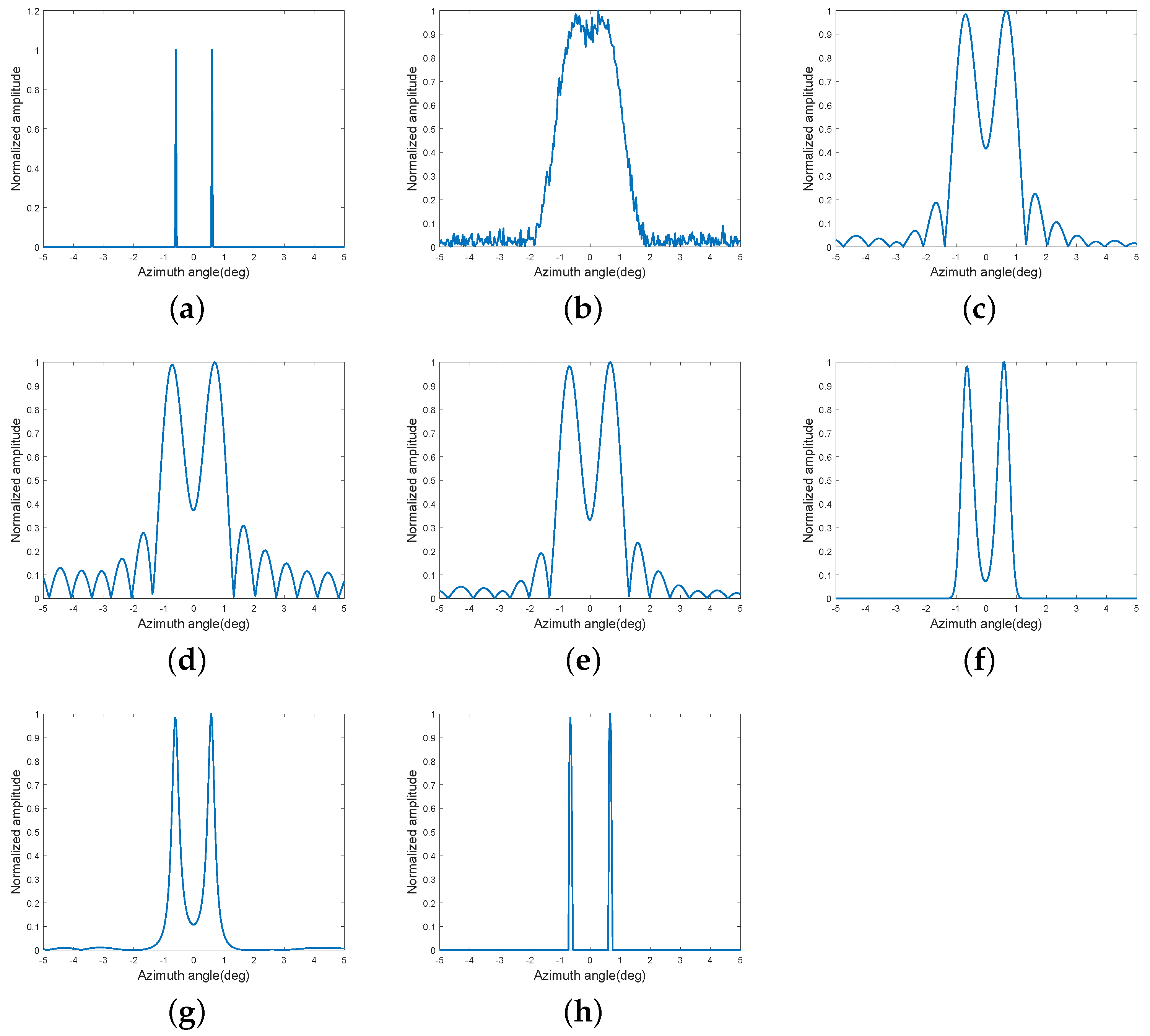
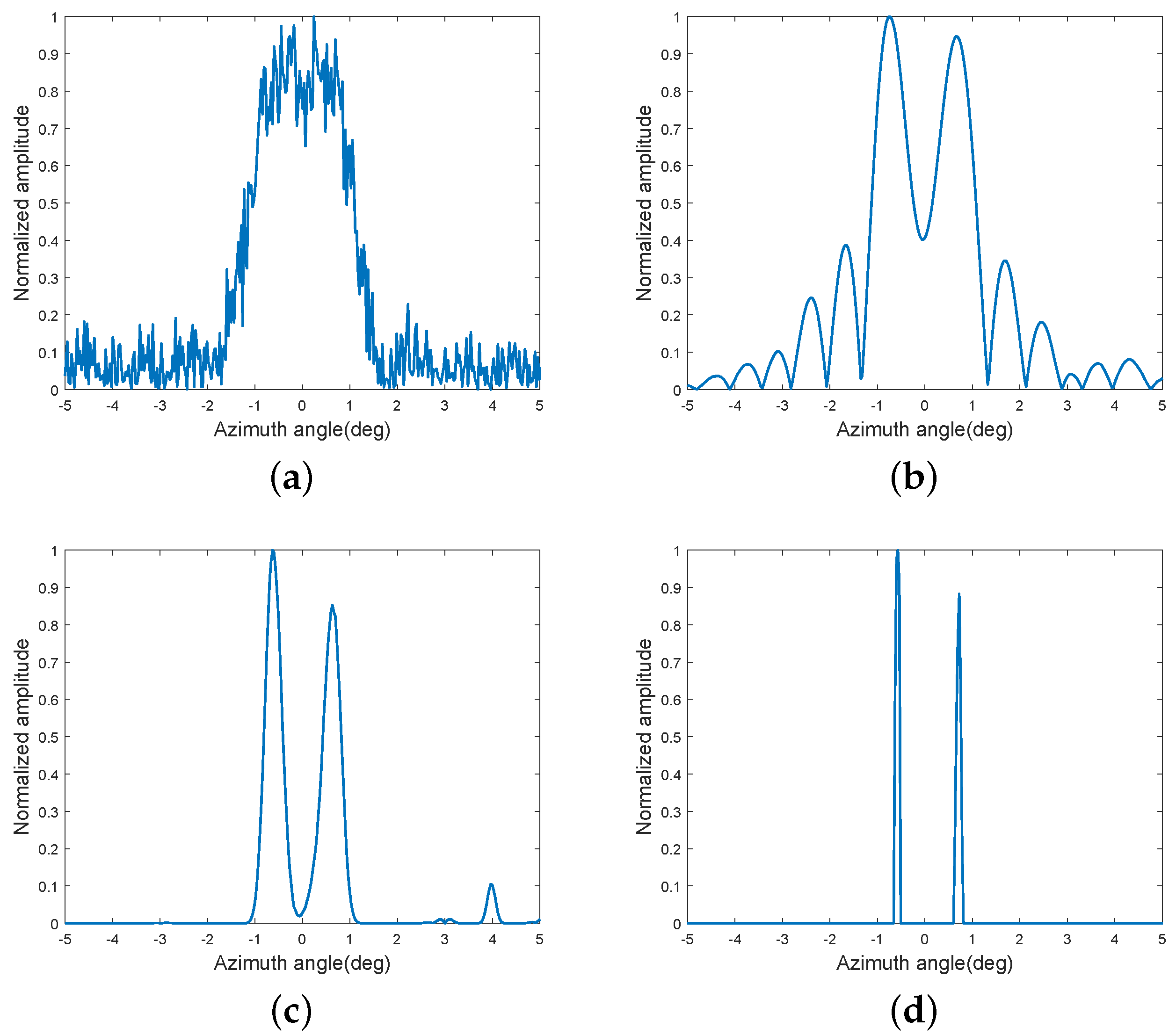
4. Simulation Results for Super-Resolution Algorithms

In this section, simulation results are given to verify the performance of the proposed method. The proposed MSL0 method was compared with the Tikhonov regularization method [26], truncated singular value decomposition (TSVD) method [27], Wiener filter method [28], sparse regularization method [20], and IAA [21]. We compared the super-resolution imaging performance and computational efficiency of the six methods through point simulation.

To quantify and compare the super-resolution performance of these six methods, we applied the structure similarity index measure (SSIM) [29] and the mean square error (MSE) [30].

The SSIM is defined as follows:

$$\mathrm{SSIM}=\frac{2\rho (\widehat{\mathbf{x}},\mathbf{x})·(2u_{\widehat{\mathbf{x}}}·u_{\mathbf{x}})}{({u_{\widehat{\mathbf{x}}}}^2+{u_{\mathbf{x}}}^2)({{\sigma }_{\widehat{\mathbf{x}}}}^2+{{\sigma }_{\mathbf{x}}}^2)},$$

(16)

where $u_{\mathbf{x}},u_{\widehat{\mathbf{x}}}$ and ${\sigma }_{\mathbf{x}},{\sigma }_{\widehat{\mathbf{x}}}$ are the mean and standard deviation of the vectors $\mathbf{x}$ and $\widehat{\mathbf{x}}$, respectively, and $\rho (\widehat{\mathbf{x}},\mathbf{x})$ represents the correlation coefficients corresponding to the vectors $\mathbf{x}$ and $\widehat{\mathbf{x}}$, respectively. The SSIM is a quantitative measure between the super-resolution imaging result and the target true scene. The value of the SSIM ranges between −1 and 1, where 1 indicates that the super-resolution imaging result is identical to the target true scene. A larger SSIM value indicates better super-resolution performance.

The MSE is used to measure the relative error between the super-resolution imaging result and the target true distribution, which is defined as

$$\mathrm{MSE}=\frac{1}{MN}∥\widehat{\mathbf{x}}-\mathbf{x}∥,$$

(17)

where M and N denote the range cell and azimuth cell, respectively.

For the simulations, we adopted the ideal $sin\mathrm{c}$ antenna pattern and considered additive white Gaussian noise. The main simulation parameters are listed in

Table 1. Simulation parameters for the radar system.

Parameter	Value
Carrier frequency	10 GHz
LFM bandwidth	75 MHz
LFM timewidth	2 $\mathsf{\mu }$s
Antenna beamwidth	3°
Antenna scanning velocity	30°/s
Scanning scope in azimuth	−10° to 10°
Pulse repetition frequency	1000 Hz

. Our point targets, as shown in Figure 4a, were located at $-0.6°$ and $+0.6°$ with normalized amplitudes of 1. As shown in Figure 4b, as the interval between the two targets was narrower than the antenna beamwidth, the echoes of the targets were mixed in the azimuth dimension. The results of the Tikhonov regularization, TSVD, and Wiener filtering methods are presented in Figure 4c–e, which show limited resolution improvements. The sparse regularization method and the IAA, as shown in Figure 4f,g, respectively, resolved the two targets to a certain extent, but their super-resolution performance was weaker than that of the MSL0 method, as shown in Figure 4h.

Table 2. Comparison of various imaging indices.

Method	SSIM	MSE	Computation Time(s)
Tikhonov regularization	0.3400	$9.9\times {10}^{-3}$	0.096
TSVD	0.2102	$10.3\times {10}^{-3}$	0.093
Wiener filter	0.3141	$9.6\times {10}^{-3}$	0.062
Sparse regularization	0.8878	$6.8\times {10}^{-3}$	0.556
IAA	0.6658	$5.4\times {10}^{-3}$	0.873
MSL0 method	0.9623	$3.8\times {10}^{-3}$	0.114

provides a comparison of the various imaging indices, where the computation times are reported from tests using Matlab 2020a on an AMD Ryzen5 4500U with 16 GB of RAM. From the simulation parameters in Table 1, the dimensions of the matrices involved can be calculated: the echo matrix y has a size of $667\times 1$, whereas the antenna measurement matrix H has a size of $667\times 667$. As shown in Table 2, the MSL0 method obtained the largest SSIM and the smallest MSE, indicating that its super-resolution performance was superior to that of the other methods. Furthermore, compared with the sparse regularization method and the IAA, the proposed method exhibited a certain advantage in terms of computation speed.

5. Influence of the SNR on the Imaging Results and Target Location Performance

This section discusses the influence of the SNR on the imaging results and target location performance. Here, we only consider the Tikhonov regularization method, sparse regularization method, and proposed method for comparison.

5.1. Influence of SNR on Imaging Results

To explore the influence of the SNR on the imaging results, we present the imaging results under low SNR conditions (10 and 5 dB). The target true scene and simulation parameter settings were the same as in the point simulation in the previous section. In Figure 5, it can be seen that when the SNR was 10 dB, the sidelobes in the Tikhonov regularization method became strong. The sparse regularization method began to produce significant sidelobes, whereas the proposed method maintained an extremely low sidelobe amplitude. When the SNR was 5 dB, as shown in Figure 6, the sidelobe amplitude of the Tikhonov regularization method was further enhanced. Both the sparse regularization method and MSL0 method produced obvious sidelobes, but those of the sparse regularization method were higher. Therefore, as the SNR decreased, stronger sidelobes were generated in the super-resolution result. Compared to the traditional methods, the SNR had the least influence on the imaging result of the proposed MSL0 method.

5.2. Influence of SNR on Target Location Performance

In this subsection, we discuss the effect of the SNR on the target location performance. We first defined the target location error (TLE), as depicted in Figure 7a; that is, we selected the peaks in the super-resolution result as the target localization result [31,32]. The TLE is calculated as

$$\mathrm{TLE}=\mathrm{abs}({\theta }_1+0.6)+\mathrm{abs}({\theta }_2-0.6),$$

(18)

where ${\theta }_1$ and ${\theta }_2$ are the angles of the left and right peaks in the super-resolution imaging results, respectively.

To examine the influence of the SNR on target localization performance, we conducted 10 Monte Carlo simulations to reduce the influence of randomness and then calculated the average of the 10 location errors. The TLE curves under different SNRs are shown in Figure 7b; with an increase in the SNR, the TLE decreased. The error curve of the proposed MSL0 method was always lower compared to that of the traditional methods; thus, MSL0 is superior to the traditional methods in terms of target location performance.

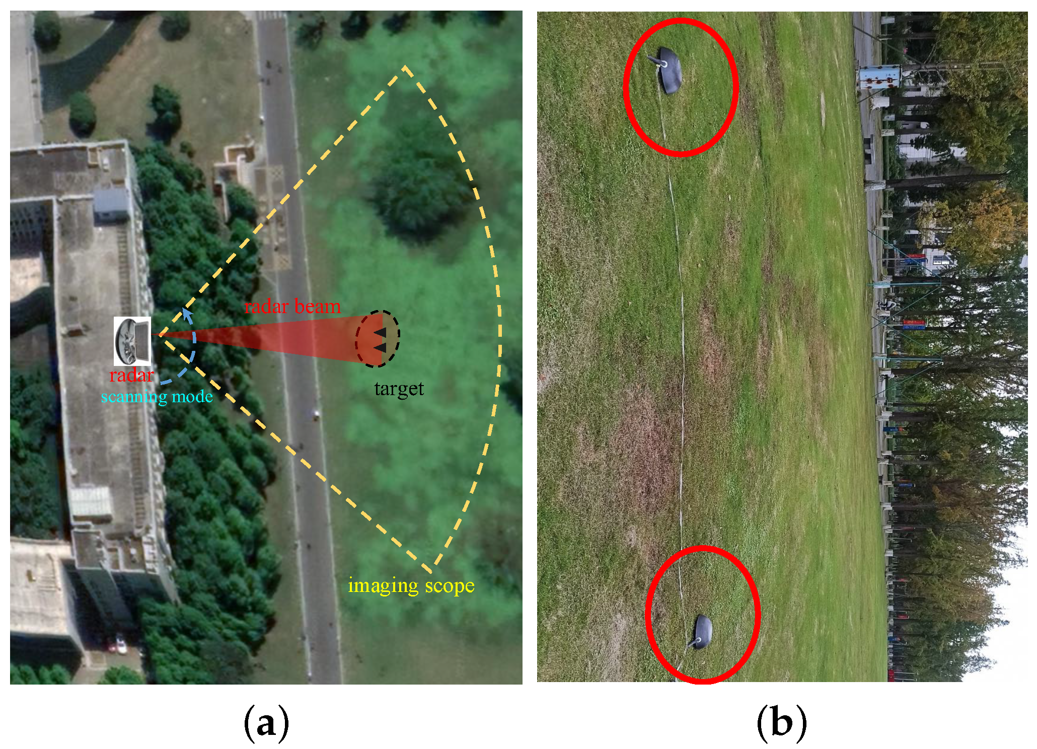
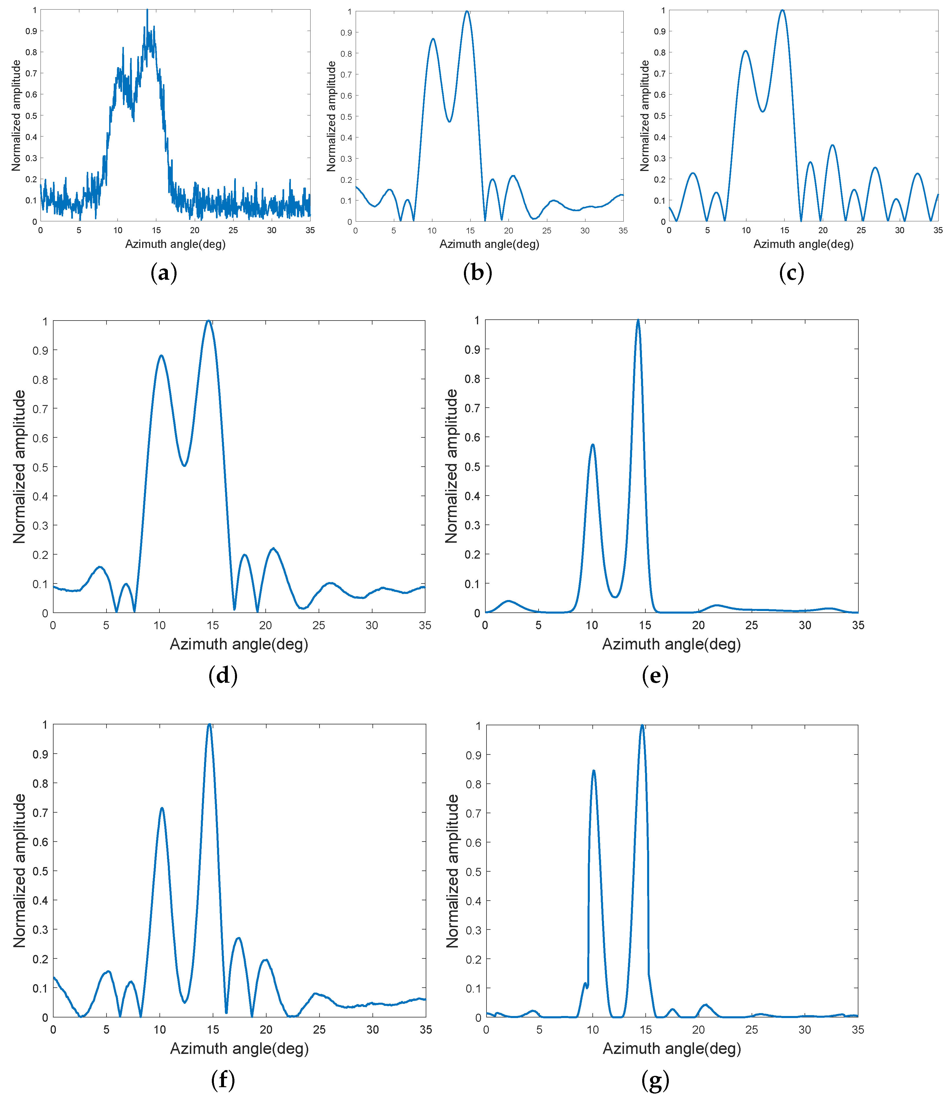
6. Experimental Data Results

Next, experimental data were applied to validate the super-resolution performance of the six considered algorithms. The experiment was carried out at the University of Electronic Science and Technology of China, Chengdu, China. In this experiment, the radar was fixed on top of a building, as shown in Figure 8a, and the targets were the two corner reflectors on the lawn in the radar forward-looking area shown in Figure 8b. The main parameters of the radar system are listed in

Table 3. Radar system parameters for experimental data collection.

Parameter	Value
Carrier frequency	30.75 GHz
LFM bandwidth	200 MHz
LFM timewidth	1 $\mathsf{\mu }$s
Antenna beamwidth	4°
Antenna scanning velocity	60°/s
Scanning scope in azimuth	$-35°$ to 35°
Pulse repetition frequency	4000 Hz
Pitch angle	$13°$

.

After collecting the echoes, we used different super-resolution methods to process the echo data using the Matlab 2020a software. The echoes of the two corner reflectors and the corresponding super-resolution processing results are marked with red ovals in Figure 9. Figure 9a depicts the real beam echo after pulse compression, which exhibited coarse resolution. The results for the Tikhonov regularization, TSVD, and Wiener filter methods are shown in Figure 9b–d. Visually, their resolution improvement effects were restricted. The results of the sparse regularization method and the IAA are presented in Figure 9e,f, where the two corner reflectors can be distinguished; however, some shadows between the two targets can be observed. Because of its superior super-resolution performance, the proposed MSL0 method achieved better shade-free processing results, as shown in Figure 9g.

The profile results in Figure 10 show that the Tikhonov regularization, TSVD, and Wiener filtering methods exhibited limited resolution improvement effects. The two targets were not completely separated by the sparse regularization method and the IAA, whereas the proposed MSL0 method achieved complete separation of the two targets.

To further evaluate the experimental data processing results of the above methods, we introduced image entropy, which is commonly utilized to evaluate the overall quality of the radar imagery since entropy increases with an increase in the image blurring level [33]. From the perspective of image processing, angular super-resolution is the removal of antenna pattern blurring, which is essentially an entropy reduction process. Therefore, lower entropy indicates better super-resolution performance [19]. Image entropy is defined as

$$E=-\sum _{m=1}^M\sum _{n=1}^N{p}_{m,n}log\left(p_{m,n}\right),$$

(19)

where the probability distribution function is

$$p_{m,n}=\frac{\left|I_{m,n}\right|}{{\displaystyle \sum _{m=1}^M}{\displaystyle \sum _{n=1}^N}\left|I_{m,n}\right|},$$

(20)

where $I_{m,n}$ is an element of the related image.

The size of the echo matrix in this experiment was $201\times 560$.

Table 4. Comparison of results of image entropy and computational times for experimental data.

Method	Entropy	Computation Time(s)
Tikhonov regularization	6.4569	8.383
TSVD	7.2049	8.199
Wiener filter	6.2383	6.644
Sparse regularization	5.1745	50.068
IAA	6.0715	46.377
MSL0 method	3.5295	11.819

compares the results of the image entropy and computational times for the various methods. The proposed MSL0 method yielded the smallest entropy, indicating that it had the best super-resolution performance in the considered practical application scenario. In terms of execution time, the proposed MSL0 method exhibited certain advantages when compared with the sparse regularization method and the IAA.

7. Discussion

This paper presents a modified smoothed L0 norm (MSL0) algorithm to increase real aperture radar angular resolution. Through simulations and experimental data verification, it can be seen that the advantages of the MSL0 algorithm include fast running speed and better imaging performance for sparse targets. However, its disadvantage is that it is only suitable for sparse targets and may fail for extended targets or dense, complex scenarios.

In future studies, we will consider combining the proposed method with another super-resolution method, where the proposed method deals with sparse targets and the other method deals with background scenes.

8. Conclusions

This paper presents our MSL0 algorithm for sparse targets. By applying the regularization strategy, we re-designed the initial iteration value and the gradient projection calculation and introduced the hard threshold operator to prevent falling into local minima. Both simulations and experimental data show that for sparse targets, the proposed method exhibits better super-resolution performance with a faster running speed compared to the commonly used sparse regularization method and the IAA.

References

1. Jose, E.; Adams, M.; Mullane, J.S.; Patrikalakis, N.M. Predicting millimeter wave radar spectra for autonomous navigation. IEEE Sens. J. 2010, 10, 960–971. [Google Scholar] [CrossRef]
2. Milias, C.; Andersen, R.B.; Muhammad, B.; Kristensen, J.T.; Lazaridis, P.I.; Zaharis, Z.D.; Mihovska, A.; Hermansen, D.D. Uas-borne radar for autonomous navigation and surveillance applications. IEEE Trans. Intell. Transp. Syst. 2023, 24, 7215–7229. [Google Scholar] [CrossRef]
3. Gao, X.; Roy, S.; Xing, G. Mimo-sar: A hierarchical high-resolution imaging algorithm for mmwave fmcw radar in autonomous driving. IEEE Trans. Veh. Technol. 2021, 70, 7322–7334. [Google Scholar] [CrossRef]
4. Huang, Y.; Liao, G.; Zhang, Z.; Xiang, Y.; Li, J.; Nehorai, A. Sar automatic target recognition using joint low-rank and sparse multiview denoising. IEEE Geosci. Remote Sens. Lett. 2018, 15, 1570–1574. [Google Scholar] [CrossRef]
5. Huang, Y.; Liao, G.; Xu, J.; Li, J.; Yang, D. Gmti and parameter estimation for mimo sar system via fast interferometry rpca method. IEEE Trans. Geosci. Remote Sens. 2017, 56, 1774–1787. [Google Scholar] [CrossRef]
6. Jia, Y.; Cui, G.; Kong, L.; Yang, X. Multichannel and multiview imaging approach to building layout determination of through-wall radar. IEEE Geosci. Remote Sens. Lett. 2013, 11, 970–974. [Google Scholar] [CrossRef]
7. Tang, Q.; Li, J.; Wang, L.; Jia, Y.; Cui, G. Multipath imaging for nlos targets behind an l-shaped corner with single-channel uwb radar. IEEE Sens. J. 2021, 22, 1531–1540. [Google Scholar] [CrossRef]
8. Valencia, E.; Camps, A.; Rodriguez-Alvarez, N.; Park, H.; Ramos-Perez, I. Using gnss-r imaging of the ocean surface for oil slick detection. IEEE J. Sel. Top. Appl. Earth Obs. Remote Sens. 2012, 6, 217–223. [Google Scholar] [CrossRef]
9. Du, L.; Liu, H.; Bao, Z.; Zhang, J. Radar automatic target recognition using complex high-resolution range profiles. IET Radar Sonar Navig. 2007, 1, 18–26. [Google Scholar] [CrossRef]
10. Kirscht, M.; Mietzner, J.; Bickert, B.; Dallinger, A.; Hippler, J.; Meyer-Hilberg, J.; Zahn, R.; Boukamp, J. An airborne radar sensor for maritime and ground surveillance and reconnaissance—Algorithmic issues and exemplary results. IEEE J. Sel. Top. Appl. Earth Obs. Remote Sens. 2015, 9, 971–979. [Google Scholar] [CrossRef]
11. Xu, G.; Xing, M.; Zhang, L.; Liu, Y.; Li, Y. Bayesian inverse synthetic aperture radar imaging. IEEE Geosci. Remote Sens. Lett. 2011, 8, 1150–1154. [Google Scholar] [CrossRef]
12. Zhang, Y.; Huang, Y.; Zha, Y.; Yang, J. Superresolution imaging for forward-looking scanning radar with generalized gaussian constraint. Prog. Electromagn. Res. 2016, 46, 1–10. [Google Scholar] [CrossRef]
13. Chen, H.; Li, M.; Zhang, P.; Liu, G.; Jia, L.; Wu, Y. Resolution enhancement for doppler beam sharpening imaging. Iet Radar Sonar Navig. 2015, 9, 843–851. [Google Scholar] [CrossRef]
14. Zhang, Y.; Wan, Q.; Huang, A.-M. Localization of narrow band sources in the presence of mutual coupling via sparse solution finding. Prog. Electromagn. Res. 2008, 86, 243–257. [Google Scholar] [CrossRef]
15. Bai, F.; Franchois, A.; Pizurica, A. 3D microwave tomography with Huber regularization applied to realistic numerical breast phantoms. Prog. Electromagn. Res. 2016, 155, 75–91. [Google Scholar] [CrossRef]
16. Chen, D.; Zhu, S.; Cao, X.; Zhao, F.; Liang, J. X-ray luminescence computed tomography imaging based on x-ray distribution model and adaptively split bregman method. Biomed. Opt. Express 2015, 6, 2649–2663. [Google Scholar] [CrossRef] [PubMed]
17. Pu, T.; Tong, N.; Feng, W.; Wan, P.; Hu, X. Mimo radar sparse recovery imaging with wideband interference prediction. Remote Sens. 2022, 14, 3774. [Google Scholar] [CrossRef]
18. Alonso, M.T.; López-Dekker, P.; Mallorquí, J.J. A novel strategy for radar imaging based on compressive sensing. IEEE Trans. Geosci. Remote Sens. 2010, 48, 4285–4295. [Google Scholar] [CrossRef]
19. Chen, H.; Li, Y.; Gao, W.; Zhang, W.; Sun, H.; Guo, L.; Yu, J. Bayesian forward-looking superresolution imaging using doppler deconvolution in expanded beam space for high-speed platform. IEEE Trans. Geosci. Remote Sens. 2021, 60, 5105113. [Google Scholar] [CrossRef]
20. Tuo, X.; Zhang, Y.; Huang, Y.; Yang, J. A fast sparse azimuth super-resolution imaging method of real aperture radar based on iterative reweighted least squares with linear sketching. IEEE J. Sel. Top. Appl. Earth Obs. Remote Sens. 2021, 14, 2928–2941. [Google Scholar] [CrossRef]
21. Yardibi, T.; Li, J.; Stoica, P.; Xue, M.; Baggeroer, A.B. Source localization and sensing: A nonparametric iterative adaptive approach based on weighted least squares. IEEE Trans. Aerosp. Electron. Syst. 2010, 46, 425–443. [Google Scholar] [CrossRef]
22. Mohimani, H.; Babaie-Zadeh, M.; Jutten, C. A fast approach for overcomplete sparse decomposition based on smoothed l0 norm. IEEE Trans. Signal Process. 2009, 57, 289–301. [Google Scholar] [CrossRef]
23. Zhang, S.; Dong, G.; Kuang, G. Superresolution downward-looking linear array three-dimensional sar imaging based on two-dimensional compressive sensing. IEEE J. Sel. Top. Appl. Earth Obs. Remote Sens. 2016, 9, 2184–2196. [Google Scholar] [CrossRef]
24. Nazari, M.; Mehrpooya, A.; Bastani, M.H.; Nayebi, M.; Abbasi, Z. High-dimensional sparse recovery using modified generalised sl0 and its application in 3D isar imaging. IET Radar Sonar & Navig. 2020, 14, 1267–1278. [Google Scholar]
25. Jun-Jie, F.; Zhang, G.; Fang-Qing, W. Mimo radar imaging based on smoothed l 0 norm. Math. Probl. Eng. 2015, 2015, 841986. [Google Scholar]
26. Gambardella, A.; Migliaccio, M. On the superresolution of microwave scanning radiometer measurements. IEEE Geosci. Remote Sens. Lett. 2008, 5, 796–800. [Google Scholar] [CrossRef]
27. Randazzo, A.; Ponti, C.; Fedeli, A.; Estatico, C.; D’Atanasio, P.; Pastorino, M.; Schettini, G. A through-the-wall imaging approach based on a tsvd/variable-exponent lebesgue-space method. Remote Sens. 2021, 13, 2028. [Google Scholar] [CrossRef]
28. Palsson, F.; Sveinsson, J.R.; Ulfarsson, M.O.; Benediktsson, J.A. Mtf-based deblurring using a wiener filter for cs and mra pansharpening methods. IEEE J. Sel. Top. Appl. Earth Obs. Remote Sens. 2016, 9, 2255–2269. [Google Scholar] [CrossRef]
29. Wang, Z.; Bovik, A.C.; Sheikh, H.R.; Simoncelli, E.P. Image quality assessment: From error visibility to structural similarity. IEEE Trans. Image Process. 2004, 13, 600–612. [Google Scholar] [CrossRef]
30. Li, W.; Li, M.; Zuo, L.; Chen, H.; Wu, Y.; Zhuo, Z. A computationally efficient airborne forward-looking super-resolution imaging method based on sparse bayesian learning. IEEE Trans. Geosci. Remote Sens. 2023, 61, 5102613. [Google Scholar] [CrossRef]
31. Wu, Y.; Zhang, Y.; Mao, D.; Huang, Y.; Yang, J. Sparse super-resolution method based on truncated singular value decomposition strategy for radar forward-looking imaging. J. Appl. Remote Sens. 2018, 12, 035021. [Google Scholar]
32. Zhang, Y.; Zhang, Y.; Huang, Y.; Yang, J. A sparse bayesian approach for forward-looking superresolution radar imaging. Sensors 2017, 17, 1353. [Google Scholar] [CrossRef]
33. Long, T.; Lu, Z.; Ding, Z.; Liu, L. A dbs doppler centroid estimation algorithm based on entropy minimization. IEEE Trans. Geosci. Remote Sens. 2011, 49, 3703–3712. [Google Scholar] [CrossRef]
Figure 2. Comparison of an antenna pattern in different domains: (a) Antenna pattern in the azimuthal time domain and (b) antenna pattern in the azimuthal frequency domain.
Remotesensing 16 00012 g002
Figure 3. Schematic diagram of approximate L 0 norm function f σ ( x ) with three values of σ .
Remotesensing 16 00012 g003
Figure 4. Point simulation results (SNR = 20 dB): (a) Target true scene; (b) Real beam echo; (c) Tikhonov regularization method; (d) TSVD method; (e) Wiener filter method; (f) Sparse regularization method; (g) IAA; (h) MSL0 method.
Remotesensing 16 00012 g004
Figure 5. Point simulation results (SNR = 10 dB): (a) Real beam echo; (b) Tikhonov regularization method; (c) Sparse regularization method; (d) MSL0 method.
Remotesensing 16 00012 g005
Figure 6. Point simulation results (SNR = 5 dB): (a) Real beam echo; (b) Tikhonov regularization method; (c) Sparse regularization method; (d) MSL0 method.
Remotesensing 16 00012 g006
Figure 7. Influence of SNR on target location performance: (a) Definition of target location error; (b) Target location error curve.
Remotesensing 16 00012 g007
Figure 8. (a) Schematic diagram of the experimental scene; (b) The locations of the corner reflectors.
Remotesensing 16 00012 g008
Figure 9. Experimental data processing results: (a) Real beam echo after pulse compression; (b) Tikhonov regularization method; (c) TSVD method; (d) Wiener filter method; (e) Sparse regularization method; (f) IAA; (g) MSL0 method.
Remotesensing 16 00012 g009
Figure 10. Experimental data processing profiles: (a) Real beam echo; (b) Tikhonov regularization method; (c) TSVD method; (d) Wiener filter method; (e) Sparse regularization method; (f) IAA; (g) MSL0 method.
Remotesensing 16 00012 g010