Article

DF-UHRNet: A Modified CNN-Based Deep Learning Method for Automatic Sea Ice Classification from Sentinel-1A/B SAR Images

College of Computer Science & Technology, Qingdao University, Qingdao 266071, China
*
Author to whom correspondence should be addressed.
Remote Sens. 2023, 15(9), 2448; https://doi.org/10.3390/rs15092448
Submission received: 17 March 2023 / Revised: 3 May 2023 / Accepted: 4 May 2023 / Published: 6 May 2023
(This article belongs to the Section AI Remote Sensing)

Abstract

:
With the goal of automatic sea ice mapping during the summer sea ice melt cycle, this study involved designing a fully automatic sea ice segmentation method based on a deep learning semantic segmentation network applicable to summer SAR images, which achieved high accuracy and the fully automatic extraction of sea ice segmentation during the summer ice melt cycle by optimizing the process, improving the pixel-level semantic segmentation network, and introducing high-resolution sea ice concentration features. Firstly, a convolution-based, high-resolution sea ice concentration calculation method is proposed and was applied to the deep learning task. Secondly, the proposed DF-UHRNet network was improved upon by designing high- and low-level fusion modules, introducing an attention mechanism, and reducing the number of convolution layers and other operations, and it can effectively fuse high- and low-scale semantic features and global contextual information based on reducing the overall number of network parameters, enabling it to achieve pixel-level classification. The results show that this method meets the needs associated with the automatic mapping and high-precision classification of thin ice, one-year ice, open water, and multi-year ice and effectively reduces the model size.

Graphical Abstract

1. Introduction

Sea ice covers approximately 7% to 15% of the ocean and is the most important component of the global cryosphere [1]. With global warming increasing in recent years, the areas occupied by different categories of sea ice have decreased to differing degrees [2], which has provided conditions for seasonal alterations to the Arctic navigation channel. The complex sea ice conditions in Arctic waters seriously affect the navigability of the Arctic seaway, especially during the summer sea ice melt and freeze periods, during which the sea ice conditions are serious. At different ice levels, ships have different means of quantifying navigational risk, such as by using the POLARIS system proposed by the International Maritime Organization (IMO) based on sea ice concentration and sea ice category development stage characteristics [3], which all require prior data. Sea ice information, including regarding the sea ice type and sea ice concentration of a region, needs to be obtained in advance. Therefore, sea ice classification during Arctic sea ice monitoring is important and helpful when assessing ice conditions, undertaking sea ice forecasting, and conducting polar research.
In recent years, new technologies and methods have emerged for Arctic cryosphere detection. Satellites such as the GNSS-R have a low launch cost and can be used to achieve the low-cost, high-temporal resolution detection of the above-mentioned geophysical elements through the implementation of a highly promising constellation network observation program. Many scholars have carried out related research, for example, via sea ice thickness [4,5] and sea ice concentration [6] monitoring missions. Moreover, the use of synthetic aperture radar (SAR) images to extract sea ice types is currently the main approach used in research. Traditional machine learning-based sea ice classification methods extract features to distinguish sea ice types based on backscattering, image texture, etc. For example, Liu [7] used the support vector machine and decision tree classification methods based on Radarsat-2 dual-polarization experimental data to obtain open seawater and flat ice information by calculating sea ice textural feature classification maps. Zhang proposed a method based on a combination of the Kalman filter, a gray-level concurrence matrix, and the SVM algorithm to classify SAR images. Wang [8] proposed an attribute difference decision tree classification method to be used in considering the original multi-polarization attribute features of images, which improved the accuracy of sea ice classification in full-polarization SAR images. Lohse [9] introduced a fully automatic design of a numerically optimized decision tree algorithm and demonstrated its application to sea ice classification using SAR data. In conclusion, these methods require a priori expert knowledge and complex algorithms to extract features. Further, in Arctic Sea ice classification tasks, differences in regions and seasons have a large impact on sea ice classification accuracy, which make it difficult to ensure the fast, frequent, and fully automated delivery of sea ice segmentation maps. Moreover, image classification based on traditional methods cannot extract deep-level features and often misses spatial and textural features that are beneficial for classification. In recent years, various deep learning algorithms have gradually been developed and matured, and deep learning techniques have been widely used in the fields of target detection and image semantic segmentation [10]. Further, many researchers have used deep learning-based full convolutional neural networks to extract sea ice classification information. For example, Wang [11] was the first to use deep learning convolutional neural networks (CNNs) to map sea ice concentrations in 2016 and illustrated the potential of deep learning in relation to the study of classification methods for two open ocean categories and four sea ice categories in response to the different representations of the features of different polar categories in Sentinel-1A images. De Gelis [12] applied a fully convolutional network of U-Net networks to a Sentinel-1 SAR image classification prediction task. Huang [13] applied CNN models in sea ice concentration assessments and sea ice classification experiments, resulting in an overall classification accuracy of 93% and a kappa coefficient of 0.8. Deep learning semantic segmentation methods can better tap into the deep non-linear relationships of image features and thus better extract the change patterns of data features, which can then be applied in the field of sea ice segmentation tasks. In summary, during the summer sea ice freezing and melting period, regional sea ice conditions are complex, and sea ice classification becomes a more and more difficult problem. Deep learning also has problems; for example, deep learning-based methods require a large number of labeled samples, which entails a lot of manual work, and the differences between sea ice categories are small, while their interpretation often requires the input of experienced professionals. Meanwhile, although SAR has the advantages of being all-weather and unaffected by cloudy images, the SAR data source itself has fewer feature dimensions compared with optical remote sensing and lacks rich feature information.
In this paper, remote sensing sea ice image classification in the Arctic summer is addressed using dual-polarized Sentinel-1SAR C-band images. Under the conditions related to melting sea ice, it is difficult to distinguish ice types in the C-band [14], meaning it will be important to figure out how to extract deeper feature information useful for sea ice classification using deep learning methods. This paper focuses on the optimization of the automatic summer sea ice classification process for SAR images and peri-ice map data. A high-resolution sea ice concentration feature extraction method was designed to improve sea ice classification based on SAR images of summer sea ice melt cycles. Compared with traditional sea ice concentration extraction methods, this method uses convolution operations and array computation operations to quickly and accurately complete regional high-resolution sea ice concentration feature extraction tasks. A deep learning fully convolutional neural network—the Double Fusion Module of a U-shaped High-Resolution Network (DF-UHRNet)—is also proposed. It is a semantic segmentation model combining U-Net and HRNet structures. The effective segmentation of summer sea ice was achieved by designing two fusion modules, introducing an attention mechanism, a conditional random field, and morphological post-processing modules. The specific contributions of our work are as follows:
(1)
We propose a U-shaped network architecture using the two fusion modules. Compared with the U-HRNet and HRNet networks separately, it requires fewer network parameters and can more effectively fuse neighboring scale semantic features and extensively extract global contextual information to achieve summer sea ice classification.
(2)
We designed a sea ice concentration extraction method based on the K-means clustering algorithm and convolution operation, which can extract high-resolution information regarding the sea ice concentration in the Arctic region during summer using SAR images, is faster in terms of extraction, and can obtain a better resolution compared with traditional methods.
(3)
We propose a deep learning-based process of optimization for the automatic classification of Arctic summer sea ice using SAR and ice map data, enabling the one-click extraction and identification of sea ice in the region.
The experimental results show that our method can achieve the fully automated and effective extraction of sea ice classification information from the Arctic region during summer, and the proposed model is better in all relevant experimental metrics. This study can provide sea ice segmentation maps and sea ice concentration data for the fast and accurate identification of sea ice in the summer polar route sea ice area and provide guidance for the planning and dynamic correction of polar routes. The rest of this paper is organized as follows. Section 2 describes the study area and related data and presents the high-resolution sea ice concentration calculation method and the proposed network structure. The third section presents the experiments and an analysis of the results. Finally, Section 4 provide discussions of the results and conclusions, respectively.

2. Materials and Methods

2.1. Ice Charts

This study used the weekly ice charts released by the Canadian Ice Service (CIS) as the baseline for classifying the training data and validating the test data used for the semantic segmentation of sea ice via deep learning. The CIS, an essential component of the Canadian Meteorological Service (CMS), provides sea ice charts that were compiled through in situ collection and satellite and aerial reconnaissance, which cover the five study hotspots in the North Pole. The ice charts contain one-week sea ice concentration data for the study area, the development stage of sea ice coverage in the area, and the percentage of sea ice coverage; these data not only covered our area of study but have also been proven over the years to be relatively reliable and accurate, supporting their validity.
The ice charts published by the CIS follow the sea ice classification standards of the World Meteorological Organization (WMO). The ice charts, published in the shapefile format, were extracted and matched with SAR images using Python software to obtain the original uninterpreted ice chart information. We also set corresponding reading rules, such as using sea ice development stages and proportions in determining the main sea ice types; labels for open water and land areas were also extracted based on the information on sea ice concentration and the development stages. Meanwhile, the places identified as unknown and glacial areas were cropped out as effectively as possible.

2.2. SAR Imagery

Compared with visible remote sensing and near-infrared remote sensing, the SAR images acquired by Sentinel-1 had the advantage of being unaffected by atmospheric and solar radiation; compared with passive microwave remote sensing, this approach has higher spatial resolution and can provide more details on sea ice boundaries. Further, compared with other SAR image types, it yields far more data, which are open-source and more accessible [15], and have short satellite revisit cycles. These characteristics make it widely popular among polar researchers, and it is the top choice for the extraction of sea ice classification information.
The Sentinel-1 satellite constellation is an Earth observation satellite within the European Copernicus program, consisting of two radar satellites set 180° apart. It is a two-satellite system containing Sentinel-1A and Sentinel-1B satellites, with a single satellite revisit cycle of 12 days and a shortened double satellite revisit cycle of 6 days. One of the Sentinel-1B satellites was officially determined to be offline on 6 August 2022, after it was rendered unable to transmit radar data due to anomalies in the power supply of its instruments, along with other reasons, beginning on 23 December 2021. We selected 2020 data for this study. The Sentinel-1A/B data used in this study were obtained from https://search.earthdata.nasa.gov/ (accessed on 3 May 2023) and comprise L1-level medium-resolution ground data detection product (GRDM) data, from which images had multi-look and thermal noise removed to enhance their quality.
The SWATH mode of the Sentinel-1 dual-polarization (HH/HV) product, the medium-resolution ground data detection product (GRDM), was used in this study. The product has an image width of 400 km per scene, a resolution of 100 m in terms of both distance and orientation, and a uniform pixel scale of 50 m × 50 m after resampling. All the data were dual-polarized, i.e., they underwent horizontal emission and reception (co-polarization, HH) and horizontal emission and vertical reception (cross-polarization, HV). The data were pre-processed, including via orbit correction, refined Lee denoising, radiometric calibration, and terrain correction. All data were projected into a coordinate system with a spatial resolution of 50 m.
Following filtration and space–time matching, data with spatial distributions overlapping with the weekly ice charts published by the CIS, as well as data with a time difference of less than 1 day from the ice charts, were obtained and used to extract sea ice features. Finally, more than 60 views of Sentinel-1A/B data between July and November 2020 were obtained as the training dataset. To reduce the incidence angle dependence of Sentinel-1 SAR images in the HH band, angle of incidence normalization correction was first carried out using Python software, and the images were then sliced to obtain the 256 × 256 pixel training datasets.

2.3. Description of the Study Area

The Eastern Beaufort Sea region was selected as our study area. This area of sea is located between northern Alaska and the northwestern Canadian coast, north of Banks Island, west of the Arctic islands, and east of the Chukchi Sea. In the summertime, the northern part of the sea remains heavily covered with multi-year ice that is conveyed from the central Arctic by anticyclonic Beaufort circulation [16]. In the southern part of this sea, there are areas of widely covered open sea, as well as areas of newly frozen sea ice.
During the navigable window of the Arctic shipping lanes (early August to late October), the sea ice in the Beaufort Sea area undergoes a melting, drifting, and then freezing process, producing many different types of sea ice, which can be classified using deep learning remote sensing semantic segmentation methods. The types of sea ice in this sea are complex and more typical, with almost all the WMO-defined sea ice development stages represented throughout the summer period. As shown in Figure 1, the sea ice types in this zone are mixed and disordered, but mainly comprise multi-year ice and thin ice. We classified the sea ice into four stages based on the sea ice development process defined by the WMO, which are open ocean, one-year ice, multi-year ice, and thin ice. Here, thin ice refers to the group of sea ice stages with a thickness of less than 30 cm, including new ice, Nilas ice, young ice, and gray and gray-white ice. Multi-year ice refers to the group of sea ice stages with a thickness of more than 120 cm, mainly consisting of old ice, second-year ice, and multi-year ice. Due to the low distribution of one-year ice during the summer ice melt period, we grouped both unknown developmental stages and iceberg regions into the one-year ice category. Different types of sea ice show significant differences regarding their representation in SAR images. Because the microwaves emitted by SAR are scattered more diffusely on rough surfaces, causing the sensor to receive returning microwaves from multiple directions, such surfaces appear brighter. Multi-year ice tends to have a rougher surface than one-year ice due to a variety of factors, such as sea winds and multi-year melting. Thin ice, on the other hand, is also affected by both melting and freezing during its formation, making the surface smoother, but with more widespread coverage and distributions, such as in inter-ice channels, compared to one-year ice. These factors account for the differences in color and texture between different types of sea ice.
The most typical sea ice types in each category are gray and white ice, multi-year ice, and thin one-year ice. In terms of time scale, our study focuses on the summer ice melt period, during which we found fewer one-year ice examples, and therefore, the one-year ice type was considered as a background category in our experiments.

2.4. Overall Process of Sea Ice Image Segmentation

We automated the analysis of the summer ice charts with a 50 m spatial resolution by designing a fully automated sea ice segmentation process for summer with an improved deep learning semantic segmentation technique for overall sea ice categories. The overall sea ice classification information extraction process is shown in Figure 2.
As ideal experimental data, the contents of the weekly CIS ice charts effectively reflect the sea ice categories that occur in the area during summer, but one faces several problems when these are used directly for deep learning training, including the following: (1) The CIS weekly ice charts are released every Monday, and there is thus a gap between the time of acquiring the SAR images and their actual current condition. Further, the sea ice categories during the summer melt and freeze periods change very fast, so there is often a mismatch in the boundaries of the areas. This is particularly true for the boundary between thin ice and open ocean. (2) Since the sea ice concentration information contained in the CIS weekly ice charts offers a regional average based on the segmentation results, it cannot be used as a training set. (3) A large number of ice lanes develops during the summer ice melt period for thin summer ice and multi-year ice, which are not marked on the ice maps as important sea ice characterization information, and there are obvious differences in the characterization between ice lanes with open ocean and other sea ice categories. (4) The results of the ice map interpretation are rough, and other categories of sea ice are often mixed in. To improve and optimize the classification process, we must address these problems.
The features of bright white sea ice and dark gray open water are easily distinguishable in both optical and SAR images, but making such a distinction between different sea ice types is much more difficult. Meanwhile, due to the influences of the season, temperature, and ocean circulation, the sea ice in summer is also characterized by large areas of inter-ice channels that fit into all sea ice categories, in addition to the presence of open waters, and these inter-ice channels are also an important feature to use in the classification of sea ice categories during the summer melt.
Therefore, we improved the sea ice segmentation process to enable us to better perform sea ice characterization during the Arctic ice melt period, thus ensuring the mapping results cohered more closely to the interpretation of the CIS ice charts. The whole segmentation process was divided into two parts: large-area extraction of open water and sea ice segmentation by type. In terms of the space–time mismatch between the ice maps and the source data, we kept this difference to less than 1 day, while the ice charts were released every Monday and the acquired SAR images were collected from Sunday to Monday. From the spatial point of view, the most commonly mismatched areas were found to be open ocean and various types of boundaries, and so the boundary areas were discarded.
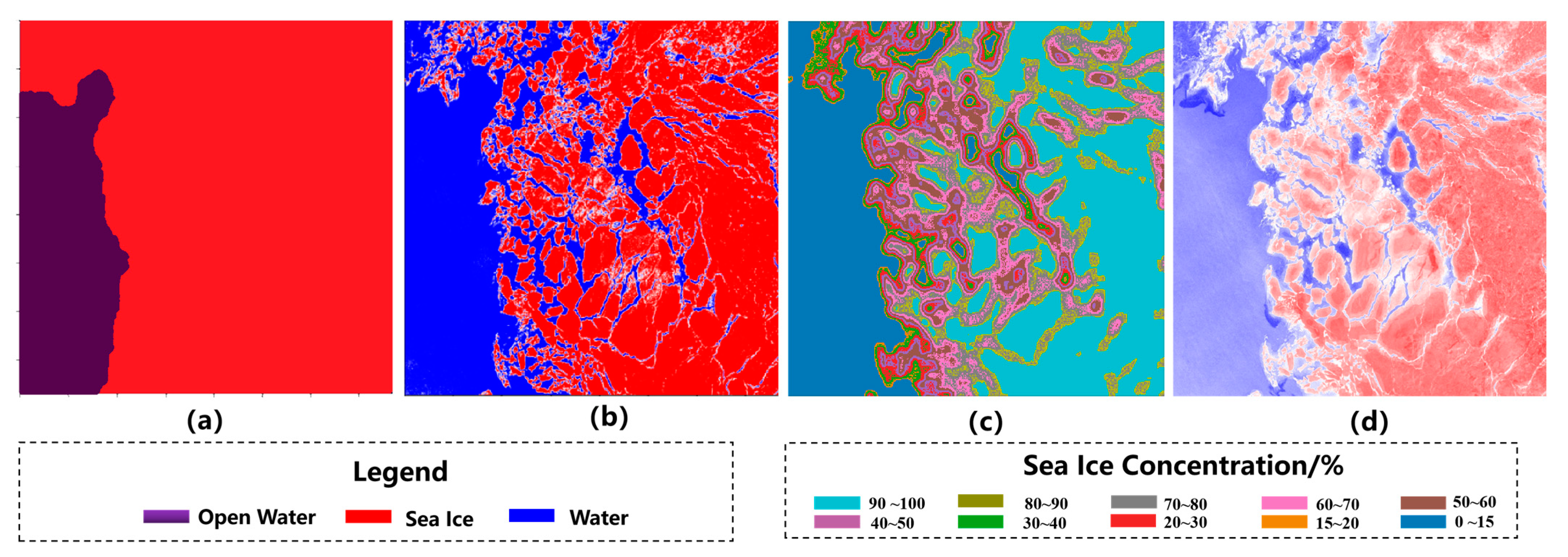
In terms of sea ice concentration, if other related products are introduced directly, not only will the difference in spatial resolution be large, but the extraction process will also become more complex. In this regard, we extracted high-resolution sea ice concentration features and first used the ice water distribution details extracted by the K-means clustering algorithm to analyze them. We then extracted further high-resolution sea ice concentration features via a sea ice concentration calculation method and then compressed and reduced the scale of the data channel via principal component analysis (PCA) [17], which was then used as the input in the sea ice classification. The extraction results are shown in Figure 3.
As regards the coarse granularity of the CIS validation data, after obtaining the sea ice classification results, the conditional random field (CRF) [18] algorithm was used to effectively remove the noise from the classification results and to optimize the boundaries. The results were then transformed into CIS-like ice maps via morphological post-processing, and the final sea ice classification results were obtained by combining the results of the two types of segmentation tasks.

2.5. Extraction of High-Resolution Sea Ice Concentration

As an important parameter reflecting the sea ice conditions in the region during the summer ice melt period, sea ice concentration can be used to infer the spatial distributional differences amongst sea ice categories to some degree. This feature is also key when considering the navigability of shipping services [19]. There are obvious differences in sea ice concentration between different sea ice categories; for example, the thin ice type tends to have a lower sea ice concentration, while that of multi-year ice is relatively higher, and one-year ice represents a kind of transition from thin ice to multi-year ice—it is rarely found in summer and has a sea ice concentration of effectively 100%.
Sea ice concentration traditionally depends on active–passive remote sensing and is defined as the percentage of sea ice area within a single image element [20], a method which generally has a low spatial resolution. Given the high resolution of SAR images, we propose an optimized high-resolution sea ice concentration calculation method, defining the average sea ice concentration within the neighboring rectangular area of a specific image element as the sea ice concentration at that point.
The whole extraction process of this method can be divided into two parts: ice water segmentation and sea ice concentration calculation. First, a regional ice water segmentation map with a 50 m spatial resolution is obtained using the K-means++ clustering algorithm [21] and land mask. Then, based on the above results, a convolution operation and array calculation are used to speed up the calculation and obtain the sea ice concentration at the same resolution as the SAR data.

2.5.1. Classification of Ice and Water

Since carrying out a fully automated sea ice classification task based on deep learning requires the preparation of a large amount of training data, this places restrictions on the selection of ice and water segmentation algorithms. It is important to ensure good robustness and extraction speed, while both ensuring algorithmic accuracy and avoiding any manual intervention in adjusting parameters. The K-means algorithm satisfies these requirements well and has been widely used in studies related to sea ice extraction and classification [22,23,24].
As an unsupervised learning method, the K-means++ algorithm does not require the aid of a priori expert knowledge and can be used to automate the extraction process. It has the advantages of low complexity and high interpretability and has good flexibility in dealing with large data samples. Compared with the traditional K-means method, K-means++ optimizes the selection of the initial class cluster center coordinates by calculating the weighted probability distribution among the class clusters, which partly solves the problem that makes K-means insufficient in the identification of weaker class clusters. However, our algorithm also has certain shortcomings, such as being more sensitive to outliers and abnormal values; the setting of the initial class values, k, and the number of iterations have a large impact on the clustering results and need to be manually pre-specified. Further, its application with non-convex data is not effective.
In this study, our goal was to accurately extract the details of regional ice water distribution, and so the selection of relevant parameters was equally important. The data were pre-normalized using the HH and HV bands’ backscattering intensities of the SAR image data, and the land areas were removed using a land mask before clustering. After applying the clustering algorithm, based on the difference in brightness between sea ice and seawater in the HV band of the SAR images, the final classification results were obtained by calculating the mean value of the clustered data in the HV band, labeling the lower ones as sea ice and the higher ones as seawater.
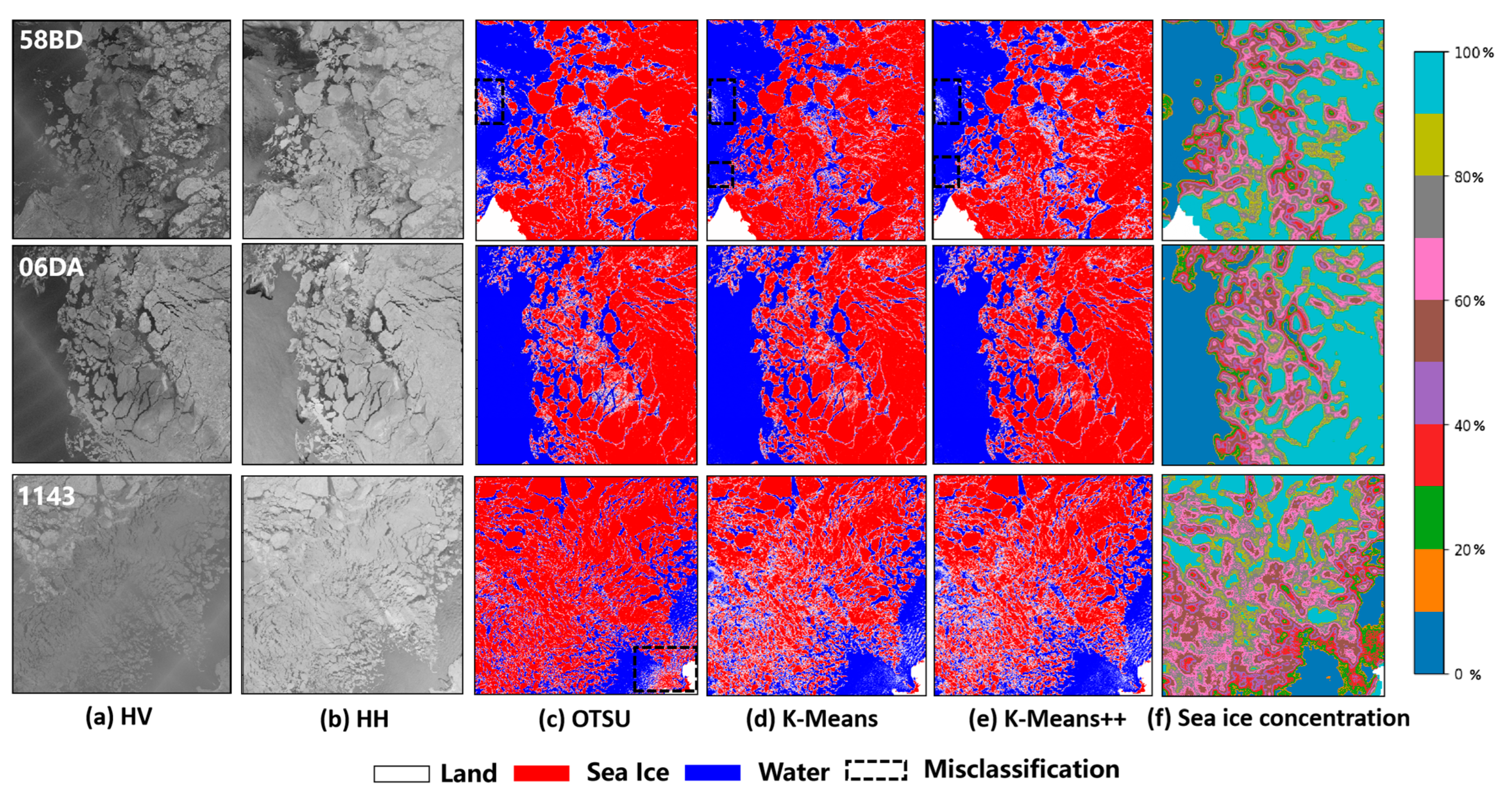
The open water in the HH band of SAR images is affected by sea wind, and the sea surface texture there is rougher, while the backscattering is enhanced, which leads to the values of ice and water brightness being similar to each other [25]. Through a large number of experimental observations, the rough seawater on the sea surface is more easily identified as sea ice when the number of clusters, K, exceeds three, and misclassification of ice and water will lead to the overestimation of ice conditions. In this regard, we set the number of clusters, K, as two for ice water extraction and compared several similar methods; the identification results are shown in Figure 4. The Otsu method yields better extraction results when the image distribution presents two peaks, but serious misclassification occurred when the ice was distributed ice and the water was uneven. While the K-means and K-means++ algorithms are similar overall in terms of their recognition of large pieces of ice, K-means++ is better applied in the recognition of details and yields more accurate data for fine and miscellaneous ice, with less noise.

2.5.2. Calculation Method of Sea Ice Concentration

In sea ice concentration calculation, the traditional method involves using a small sliding window and calculating the ratio of the number of sea ice pixels within it to the total number of pixels. This method is simple in principle, but time-consuming.
Here, we propose a fast sea ice concentration calculation method based on convolution and array operations. The convolution operation quickly counts the number of sea ice and seawater points, and array operations can be used to directly obtain the sea ice concentration data at a 50 m resolution for the whole area. The algorithm proceeds as follows:
Step 1: Segmentation maps of ice, water, and land are extracted based on the method outlined in Section 2.5.1, by identifying the land area followed by the land mask. Since sea ice concentration determination involves using the k s 2 image elements in the surrounding rectangular area to calculate the sea ice concentration value at the center point, where ks indicates the size of the convolution kernel, the edge of the image needs to be filled symmetrically in advance before carrying out the rest of the process, and the length of the filled image elements on each side is calculated as k s 2 .
Step 2: Preliminary processing of the triple classification map. Here, we set the pixel value of the sea ice point to 1 and the pixel value of seawater points to 0, while the land area is given the same pixel value as the sea ice point of 1. The first convolution operation is carried out with a convolution kernel value of 1 and convolution kernel size of ks to obtain the statistical map A l I .
Step 3: Similarly to Step 2, the land area is first given the same pixel value (0) as the seawater point, and the second convolution is carried out using a convolution kernel with a value of 1 and a size of ks to obtain the second statistical map A l w .
Step 4: Matrix operations are carried out based on Equation (2) to obtain high-resolution sea ice concentration data.
S I C = A l w A k s 2 A l w + A l I × 100 %
where ks is the kernel size—the spatial resolution of the sea ice concentration data is 50 m × ks; SIC denotes the point sea ice concentration matrix of the region; A k s 2   is the matrix containing all values; A l I is the result obtained when setting all sea ice points to 1 and seawater points to 0, treating the land region as sea ice, and performing a single convolution using a rectangle of size ks with a fixed value of 1 for the convolution kernel; and A l w is the result obtained when treating the land area as seawater and performing a single convolution using the same convolution kernel. A value of sea ice concentration between 0 and 1 is obtained by the formula, which greatly reduces the time of calculation of sea ice concentration. Any point within the result is the calculated sea ice concentration within the k s 2 pixel region adjacent to that point, and this approach thus preserves more of the details of the spatial distribution of sea ice (Figure 3c). All the convolution operations in this method use the fast Fourier transform (FFT) to optimize the computational speed [26]. This method has been shown to significantly improve computational speed, especially for convolution kernel sizes larger than 8 × 8.
Through this calculation method, the overall time required for sea ice concentration computation is reduced to 11% that of the conventional method, although the memory required is increased. The reason for this is that the time complexity of the algorithm is reduced from O n 2 , which is required for the sliding window calculation, to O n log 2 n   due to optimization using a fast Fourier transform (FFT) in the convolution operation. In terms of extraction accuracy, the calculation process does not affect the accuracy of sea ice concentration since the above calculation method uses ice and water details obtained by K-means++ clustering, which is a fast statistical process. Using this method, the efficiency of the sea ice concentration extraction task is effectively improved.
Therefore, before being used in the input network, the extracted high-resolution sea ice concentration data were fused with the features of other channels via PCA to achieve feature extraction and dimensionality reduction. The processed data are shown in Figure 3d.

2.6. Architecture of DF-UHRNet

Through multiple extensive experiments, we found that semantic segmentation networks with complex structures and deep networks are more prone to gradient vanishing and the problem of overfitting when used in this task.
In response, we develop a simple and effective Double Fusion Module of a U-shaped High-Resolution Network by improving the structure of the U-HRNet [27]. It has the advantages of U-Net-based [28] networks and the HRNet network [29] and requires fewer computational parameters compared to the U-HRNet. It also shows better results in terms of sea ice segmentation tasks. We describe the details of the DF-UHRNet network in three main areas: the main body, the attention module, and the fusion module.

2.6.1. Main Body

The main structure of the DF-UHRNet is shown in Figure 5; it is a U-shaped network structure with a symmetrical structure of encoding and decoding common to fully convolutional neural networks, which enables end-to-end semantic segmentation tasks. The U-Net-based network has certain defects. On the one hand, it employs a skip concatenation approach, which leads to a lack of efficient multi-scale features during feature fusion recovery. This gives rise to the semantic gap problem, which is exhibited by the weak extraction ability of the network in relation to feature boundaries and small objects. In sea ice segmentation problems, the morphological details of sea ice boundaries are particularly important in obtaining good segmentation accuracy. On the other hand, U-Net-based methods use CNNs to obtain information, and CNNs are often unable to make good use of global contextual information due to the limitations of their sensory field size. In this respect, our network adopts a method of improvement similar to that of the U-HRNet network by introducing a fusion module with no more than two resolution branches into the HRNet, so as to avoid the loss of feature details that occurs due to the multiple consecutive upsampling and downsampling operations undertaken in HRNet networks. The advantages of the HRNet are thus maintained, and repeated cross-resolution information transmission can be enacted by retaining multiple resolution streams. By adopting the CBAM attention mechanism, which adjusts feature computations adaptively through the channel attention mechanism and the spatial attention mechanism, it enables unnecessary computations on each resolution feature mapping to be allocated to more meaningful parts to improve the overall semantic presentation. Details can be found in Section 2.6.2.
As is shown in Figure 5, the structure of the network’s main body can be divided into nine stages, where stages 1 and 9 involve feature convolution extraction at the same resolution, while stages 2 to 8 are the fusion modules of the same resolution features, with down- and upsampling. The higher-scale semantic features that result from the fusion process in the encoding part of stages 2 to 4 are fed into the fusion module of the decoding part of stages 6 to 8 through jump connection. The lower-scale semantic features obtained after fusion are then used in the decoding part of stages 5 to 8. The semantic features of sets with four different pixel sizes—16 × 16, 32 × 32, 64 × 64, and 128 × 128—are resampled to 256 × 256 pixels, the multitude of semantic features are spliced and fused to obtain the final layer (which is the same size as the input features), the information on images with different resolutions is cross-fused, and the activation of the softmax function is then finally followed by the final output.
Since stage 5 had the strongest semantic features with the lowest resolution, unlike other fusion modules, we introduced Atreus Spatial Pyramid Pooling convolution into the deep fusion module to increase the receptive field, extract a wider range of global contextual information, and output the results directly through the deepest semantic layer in stage 5. A more useful fusion of higher-resolution semantic and lower-resolution global contextual information is obtained by concatenating high- and low-resolution networks in parallel. This enabled us to obtain multi-scale semantic information, after which the segmentation results were post-processed using conditional random fields.

2.6.2. Attention Module

Accurately identifying the open ocean is a precondition of sea ice type classification; however, summer ice lanes can provide more information relevant to sea ice classification, which can improve overall identification accuracy. As an important part of deep learning processing, the attention module has been widely used in semantic segmentation models applied to remote sensing. Simulating human perception helps the computer select the key information from the current target.
In this experiment, we wanted the feature attention to focus more on representations such as the texture and backscattering intensity of the sea ice. For this, the Convolutional Block Attention Module (CBAM) [30], which is embedded between the decoder and the encoder, helped to reconstruct the multi-scale features extracted by the encoder module and amplified the effective feature channel weights, such that the model could pay more attention to the representational features that distinguished the sea ice categories, such as spatial and texture features. The structure of the attention mechanism is shown in Figure 6.
The CBAM consists of a channel attention mechanism and a spatial attention mechanism, set up in series. The channel attention mechanism passes the input feature map through the global maximum pooling module and the global average pooling module and then feeds it into a shared network consisting of a multi-layer sigmoid mechanism and a hidden layer that scales the output features after characteristic stacking (summation operation). The result is fed into the sigmoid activation function to obtain F′, the input features that will be used for generating the spatial attention mechanism. This acts to carry out the spatial compression of the feature map, which yields a one-dimensional vector. One of two types of pooling is used to aggregate the spatial information of the feature map, which is then sent to the multi-layer perceptual machine species for parameter sharing. The channel attention features are generated by compressing the spatial dimensions of the semantic features and merging them, element by element, with the summation.
The channel attention mechanism focuses on the parts of the feature map that have the most important influence. The spatial attention mechanism, on the other hand, takes the feature map that is output by the channel attention mechanism as its input and performs cascade operations on the features extracted by global maximum pooling and global average pooling. The features obtained are convolved to produce the channel feature map, and then a new feature map F″ is obtained after processing using the sigmoid activation function, which multiplies the previous output. The final result, i.e., the features, is obtained by combining the previous feature map with these features.

2.6.3. Low-Level and High-Level Fusion Module

The fusion module within the U-HRNet network can be used to effectively fuse together the low-resolution and high-resolution semantic information, but the presence of more bottleneck blocks in the series leads to huge model parameters, which are at the same time more prone to overfitting. In this experiment, two different fusion modules were designed to extract and fuse feature information applicable to different scales and levels of semantic intensity. After using the residual module to extract features, up- and downsampling was performed, and the splicing operation was used to enact the mutual fusion of high-level and low-level features. The structure of the high-level fusion module is shown in Figure 7a and the structure of the low-level fusion module is shown in Figure 7b. Compared with the low-level fusion module, the high-level fusion module we designed mainly facilitates the extraction and fusion of stronger semantic features at small scales and introduces improved the Atreus Pyramid Pooling Convolution (ASPP) [31] for the extraction of larger-scale semantic features before fusion, which effectively expands the receptive field and can be applied to the information of the whole region. However, the selection of the convolutional expansion rate was particularly important for the ASPP module, and here, we adopted the principle of hybrid dilated convolution (HDC) to set an expansion rate that ensured that the extracted image features could be fully addressed without any voids or missing edges. This process must consider the relationship between the maximum distance between the two non-zero points used, M, and the size of the convolution kernel used, K, as shown in Equation (2):
max M i + 1 2 r i , M i + 1 2 M i + 1 2 r i , r i K
where r i   denotes the expansion rate for the expansion rate of the i-th convolution operation, which must cover all the low-level features and ensure that no convention exceeds 1. Here, convolution dilation rates of 2, 3, and 7 were chosen to enhance the receptive field such that it could cover the entire region, effectively extract sea ice features at different scales, and more effectively extract global contextual information. At the same time, we replaced the channel fusion of features in ASPP with an ADD operation, which further reduced the overall parameters.
Overall, the present network achieves the fusion of adjacent scale features by adding fusion modules to the U-Net network after each cycle of resampling. There were seven fusion modules in total, from stages 2 to 8, which could be split into two categories: the low-level fusion module and the high-level fusion module. Compared with the original U-HRNet, which extracts features of the bottleneck block four times, this network uses a single/double basic block, which can effectively reduce the number of network parameters and thus alleviate the overfitting problem. After extracting the features using the basic block, the higher-scale features were downsampled using the lower-scale features that were input for splicing and fusion to derive new lower-scale features, and similarly, the lower-scale features were upsampled with the higher-scale features that were input to derive new fused features. In stages 6 and 7 of the decoder part, the fused features that were extracted from the encoder were fused with the deep semantic features after upsampling, and the jump connections were spliced and fused with the semantic information after the upsampling of the lower-resolution features to derive the new semantic features. The high-level fusion module was used in stage 5 to output the strongest deep semantic features at the lowest scale within the network.

2.6.4. Post-Processing Process

The post-processing part of this experiment was divided into two processes: firstly, by conditional random field (CRF) and secondly, by morphological methods and a boundary relation correction.
Using full convolutional neural networks may lead to coarse segmentation. As such, the CRF instead uses an efficient inference algorithm, wherein the two edge potentials are defined by a linear combination of Gaussian kernels in an arbitrary feature space. The algorithm assigns classes to specific pixels while considering the influence of those surrounding them in order to obtain better semantic segmentation results, which can be used to effectively eliminate the fine noise that occurs and obtain optimized recognition results.
Because our experiment used CIS ice charts as the test datasets, and the granularity of CIS segmentation is coarse in addition to the optimization of training sets, we also had to undertake post-processing to ensure the results were similar to those of the ice charts. The results of the interpretation based on deep learning can be divided into two types based on their morphology—one refers to relatively concentrated areas of sea ice, which appear as large areas of ice with small pieces distributed nearby, and the second is a mixture of multiple sea ice categories, which appears as a block of dense foreground ice segmented by other sea ice types.
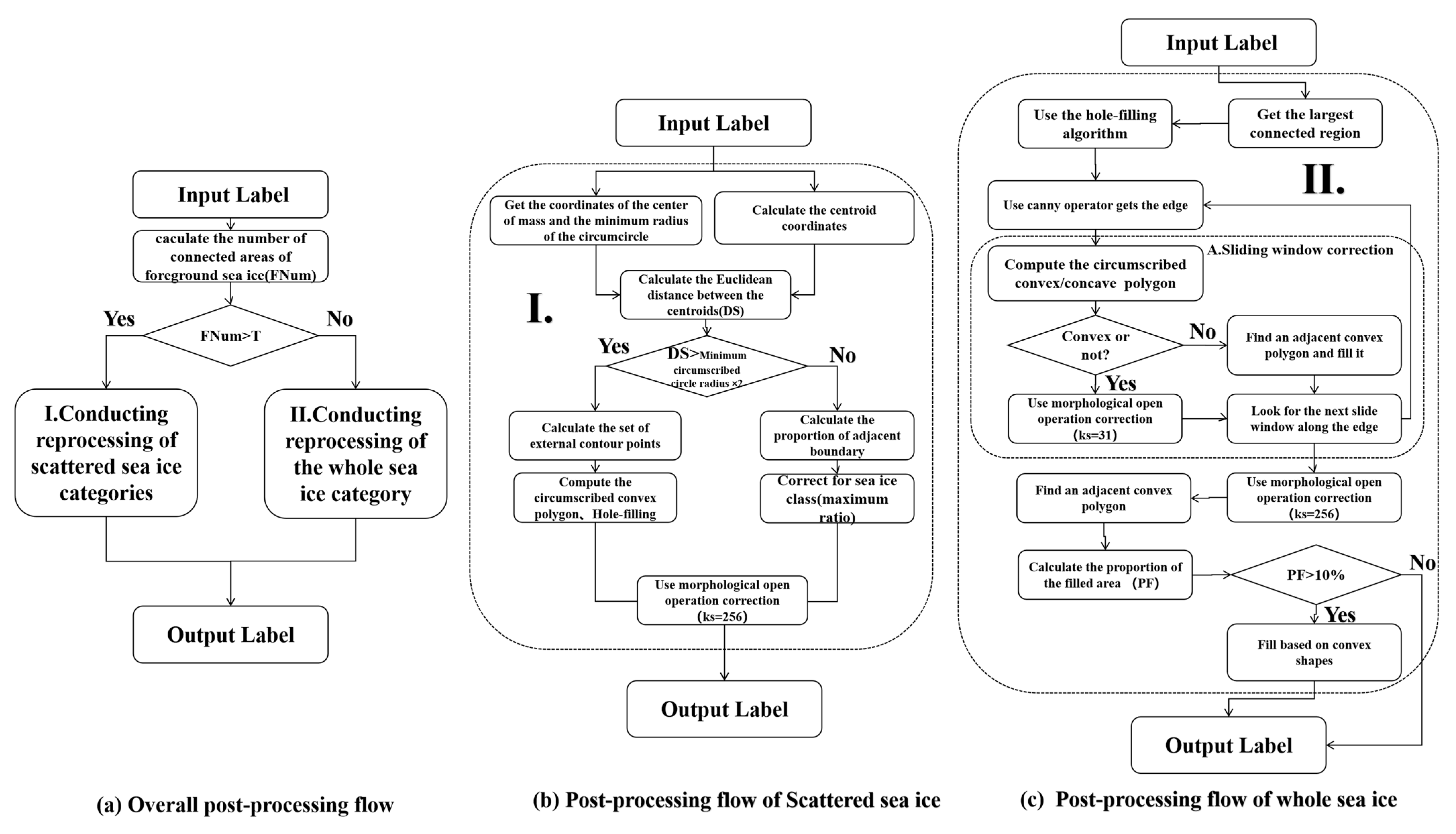
We also designed a morphology-based post-processing method for the correction step, the processing flow of which is shown in Figure 8. Among these morphologies, the classes that appeared in the foreground were seawater, multi-year ice, and thin ice (in order of post-processing priority), and the background classes were primarily other sea ice classes dominated by one-year ice. The optimization process was used to determine the foreground class of the decoded deep learning results by obtaining the number of connected regions and then setting a threshold. In the post-processing of the first category of dense sea ice, the edge details were mostly preserved, and the whole region was traversed by a sliding window (Figure 8c). For the second category, on the other hand, post-processing involved linking together the scattered foreground sea ice categories (Figure 8b), correcting the sea ice regions set at a distance from the center, and preserving as much of the edge regions as possible. This post-processing approach helps ensure that the sea ice classification results derived from deep learning are as close as possible to the results shown in the ice chart.

2.7. Accuracy Metric

To verify the effectiveness of the proposed network and the improvements made to sea ice classification, we employed evaluation metrics commonly used in the field of image semantic segmentation, including the overall accuracy, kappa coefficient, Mean Intersection Over Union (MIoU), and F 1 _ s c o r e to enact a performance analysis. We started by calculating the confusion matrix to obtain True Positives (TPs—those samples correctly predicted and judged as positive), True Negatives (TNs—those correctly predicted and judged as negative), False Positives (FPs—incorrectly predicted but judged as positive) and False Negatives (FNs—incorrectly predicted but judged as negative). Then, four evaluation metrics were calculated:
O A = T P + T N T P + F P + F N + T N
K a p p a = O A P e 1 P e    
M I o U = 1 k + 1 i = 0 k T P T P + F P + F N
F 1 _ s c o r e = 2 × T P 2 × T P + F P + F N
where OA refers to the proportion of all the correctly judged results out of the overall number, and the formula is the same as that shown in Equation (3). The Kappa coefficient is used to measure the accuracy of the image algorithm, which is defined in Equation (4). Here, P e indicates the overall and desired classification accuracy, and the closer the Kappa coefficient to 1, the more effective the segmentation. P e represents the sum of the “product of actual and predicted quantities” for all categories, divided by the “square of the total number of samples”. M I o U represents the ratio of intersection and concatenation between the segmentation and real results of a category following the segmentation algorithm, and the closer the I O U is to 1, the more effective the segmentation; the formula is the same as that shown in Equation (5). k is the number of categories classified. The F1_score measures the relationship between the segmentation results and the recall, and the formula is the same as that shown in Equation (6).

3. Experiments and Analysis

3.1. Data Selection and Usage

To filter out the features from the feature space that play a determinative role in the classification results, reducing the number of dimensions in the feature space not only reduces the time required to build the classification model effectively, but can also help avoid dimensional explosion and prevent model overfitting.
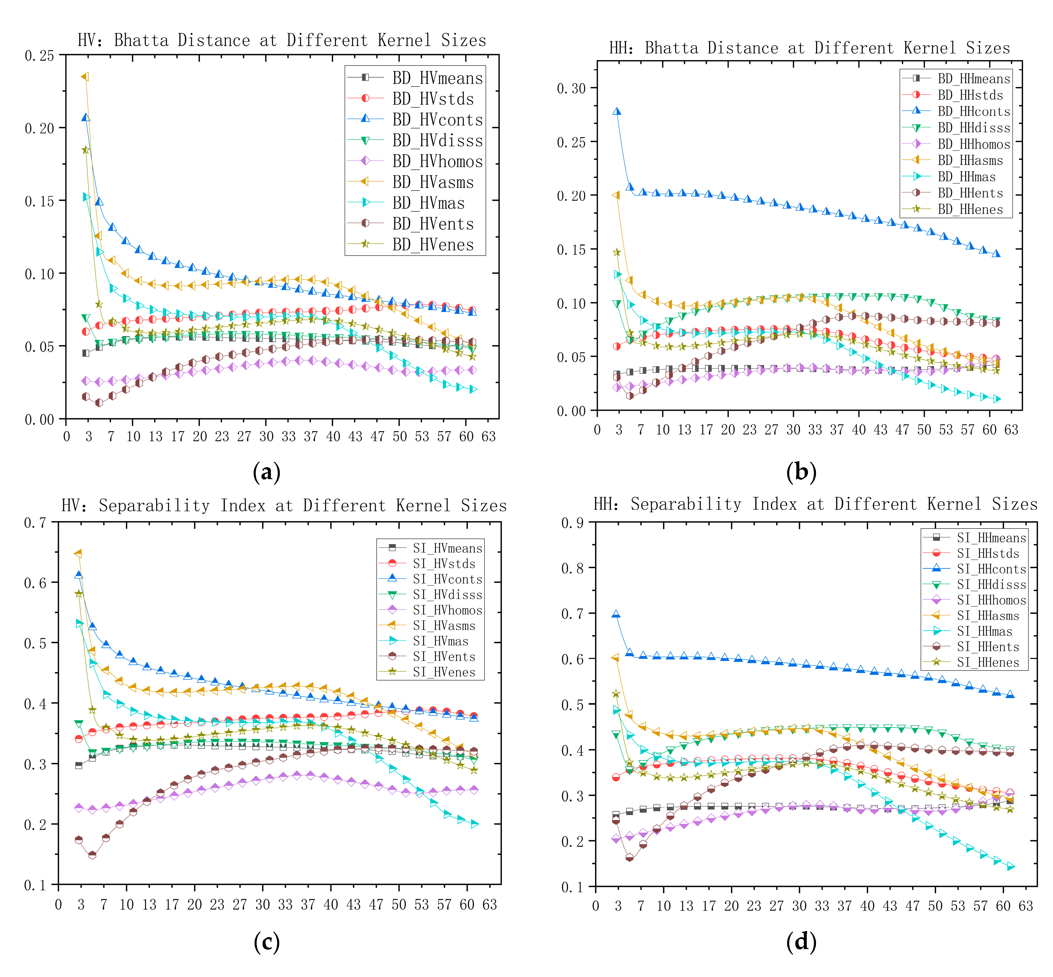
By using two types of parameters, the Bhattacharyya distance (BD) [32] and the feature separability index (SI) [33], we could provide a reference for feature selection. The feature separability index is determined by considering the point at which the mean distance between two or more types of features is greater than the standard deviation between these features, and a larger value indicates better feature separability. To determine the optimal size of the extraction window for the gray-level concurrence matrix (GLCM) texture features [34], we considered the two categories of thin ice and multi-year ice, and each texture feature was calculated using a window size of 3 × 3 to 61 × 61. As shown in Figure 9, with a sliding window size of thirty, the two types of index features reached their maximum values and showed good separability.
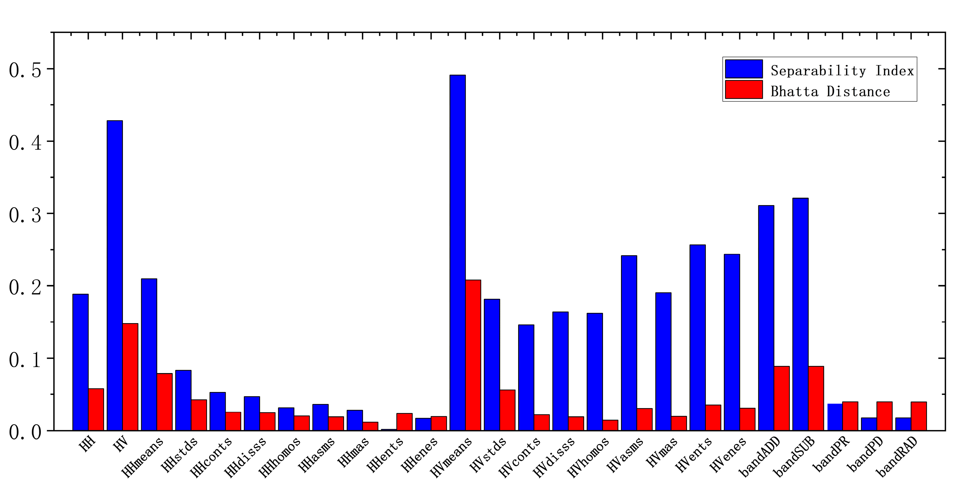
In dealing with the EW mode surface distance data within the SAR images, 2-dimensional backscattering joint coefficients, 6-dimensional band calculation features, and 18-dimensional image texture features were extracted after data pre-processing. Using the same method, the separability of the extracted 26-dimensional features was assessed, and the BD and SI parameters were calculated for these data with reference to one-year ice and multi-year ice; the comparison results are shown in Figure 10, and values with more detail can be found in Table 1. The bands with the best differentiability for both thin ice and multi-year ice were found to be σ H H 0 , σ H v 0 , HH Means, HV Means, σ H v 0 + σ H H 0 , and σ H H 0   σ H V 0 . Therefore, for the completion of the deep learning open ocean extraction task, we chose the σ H H 0 , σ H v 0 , and σ H H 0 σ H V 0 features as the training data to be input. In completing the deep learning sea ice classification task, we fused the extracted high-resolution sea ice concentration data with the σ H H 0 , σ H v 0 , σ H v 0 + σ H H 0 , and σ H H 0 σ H V 0 features (applying PCA for dimensionality reduction) to obtain the four-dimensional features that would be used as the training input. The processed features are shown in Figure 3d.

3.2. Experimental Design

A total of over 60 scenes from images taken in July–December 2020 were collected and used as training data in this experiment. Before deep learning training, operations such as the temporal matching of ice maps and SAR data and image clipping were performed. The statistics of the categories show that multi-year ice accounted for more than 80% of the data, followed by one-year ice, and the thin ice was represented at the lowest level. To balance the number of samples as effectively as possible, we used data enhancement methods (data flipping, rotating, panning, mapping, random cutting, adding noise, etc.) to broaden the data across a small number of sample categories. As shown in Table 2, in the experimental part of the sea ice classification, the number of samples in each category was kept at 4000.
In the extraction of the open water category, we performed weighted binary cross-entropy as the loss function. For the sea ice category, we used the loss function as the cross-entropy loss function. We set the training set and test set segmentation ratios to 0.7 and 0.3, respectively, and the number of training rounds was kept at 50 via the learning rate reduction mechanism (if the loss function does not decrease for five consecutive rounds, the learning rate is halved) and the early stop mechanism (if the learning rate decreases for three consecutive rounds, i.e., fifteen rounds, the training is stopped).
Due to the large size of the SAR remote sensing images, at a 50 m spatial resolution, the pixel size of the images per view reached 13,000 × 13,000, which undoubtedly placed greater requirements on the computational speed and memory of the device itself. We employed the overlapping edge elimination strategy and rotation prediction and stitched the images after setting a fixed step size for the deep learning semantic segmentation using the sliding window. In the actual sea ice extraction task, a step size of 128 and a window size of 256 were chosen for sliding window detection, a soft voting mechanism was used to superimpose the weights of each category after the sliding window, and the final category of pixel points was output based on the weight maximum.

3.3. Experimental Results

To demonstrate the effectiveness of the sea ice classification method and the application of the DF-UHRNet network therein, two comparison experiments were designed: (1) using the Grad-CAM algorithm to implement the output of the deep semantic segmentation network (we also designed DF-UHRNet ablation experiments) and (2) using the comparison of different models employed under the same experimental conditions with the same dataset against more mainstream semantic segmentation networks, such as the U-Net, HRNet, and U-HRNet, in order to verify the advantages of our algorithm.

3.3.1. Ablation Study

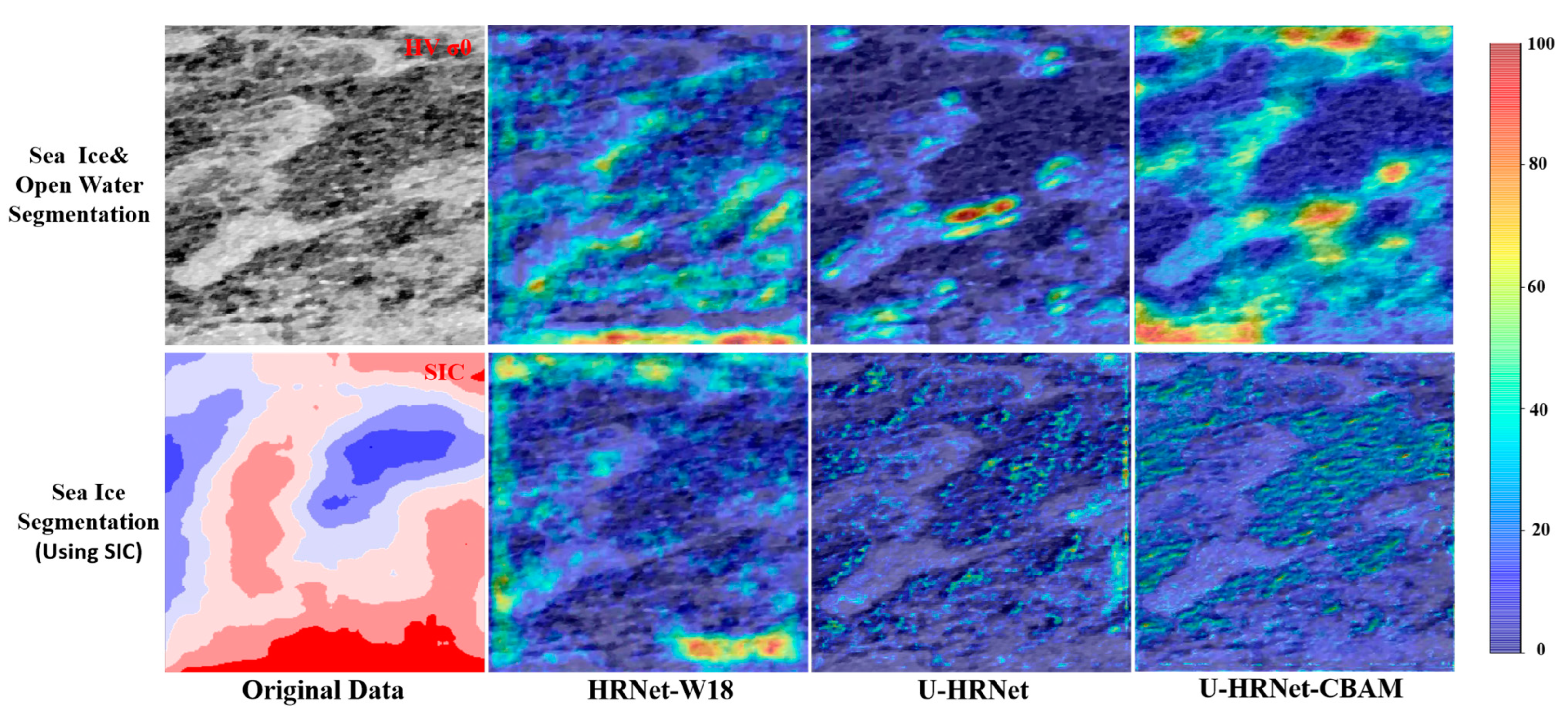
To demonstrate the effectiveness of the improvements made here to the network used for the sea ice segmentation task, an ablation experiment was designed, and the final layer of network results was visualized and output using the Grad-CAM algorithm. The Gradient-weighted Class Activation Mapping (Grad-CAM) [35] technique offers a better visual representation of the deeply connected neural network, thus yielding a view that enables a more favorable interpretation of the CNN network when performing segmentation. Using this algorithm, we could compare the results yielded before and after the introduction of the attention mechanism for two types of tasks.
In Figure 11, the first row refers to open water segmentation, where the traditional U-HRNet was used; the class activation results of this method are more focused on the sea ice region compared to the HRNet, in which attention was enhanced after the introduction of the attention mechanism of CBAM. The second row refers to the sea ice depth segmentation task. Since large inter-ice channels emerge in the summertime, and these inter-ice channels are not marked individually in the CIS peri-ice map, they are regarded as components of other categories of sea ice. They also offer important representations of each category and following the introduction of the sea ice concentration feature, the HRNet can be made to focus more on sea ice regions, i.e., regions with higher sea ice concentrations. The traditional U-HRNet approach focuses on regions with lower sea ice concentrations, where textural changes are more obvious, and the features here were enhanced after the introduction of CBAM. As such, after introducing the sea ice concentration feature, the focus of the whole network could be effectively directed towards regions with higher sea ice concentrations, and this facilitated the segmentation of the summer sea ice category, i.e., by focusing on the whole region rather than just the sea ice region. As such, the experimental effect was improved. Features derived both with and without CBAM were also introduced and were compared using Grad-CAM; we found that by introducing CBAM, attention was effectively directed towards the sea ice region, and the effect of the segmentation was thus effectively improved. Longitudinally, a given network model will differ in terms of its information, which focuses on one of two different types of segmentation tasks—open ocean recognition focuses more on identifying sea ice regions, while sea ice classification focuses on the whole representational information of the region.
To verify the effectiveness of the two fusion modules, as well as CBAM and the ASPP module, when used in sea ice classification, we conducted ablation experiments using the same training data and experimental parameters, and the results are shown in Table 3. Our model showed significant improvements compared to the HRNet and to the model using only one fusion module, the model with CBAM, that with CRF post-processing, and that with high-resolution sea ice concentration features, especially in the MIoU parameters, which improved by 13.7%, 12.9%, 0.6%, 7.1%, and 4.8%, respectively.

3.3.2. Comparing Experiment Results

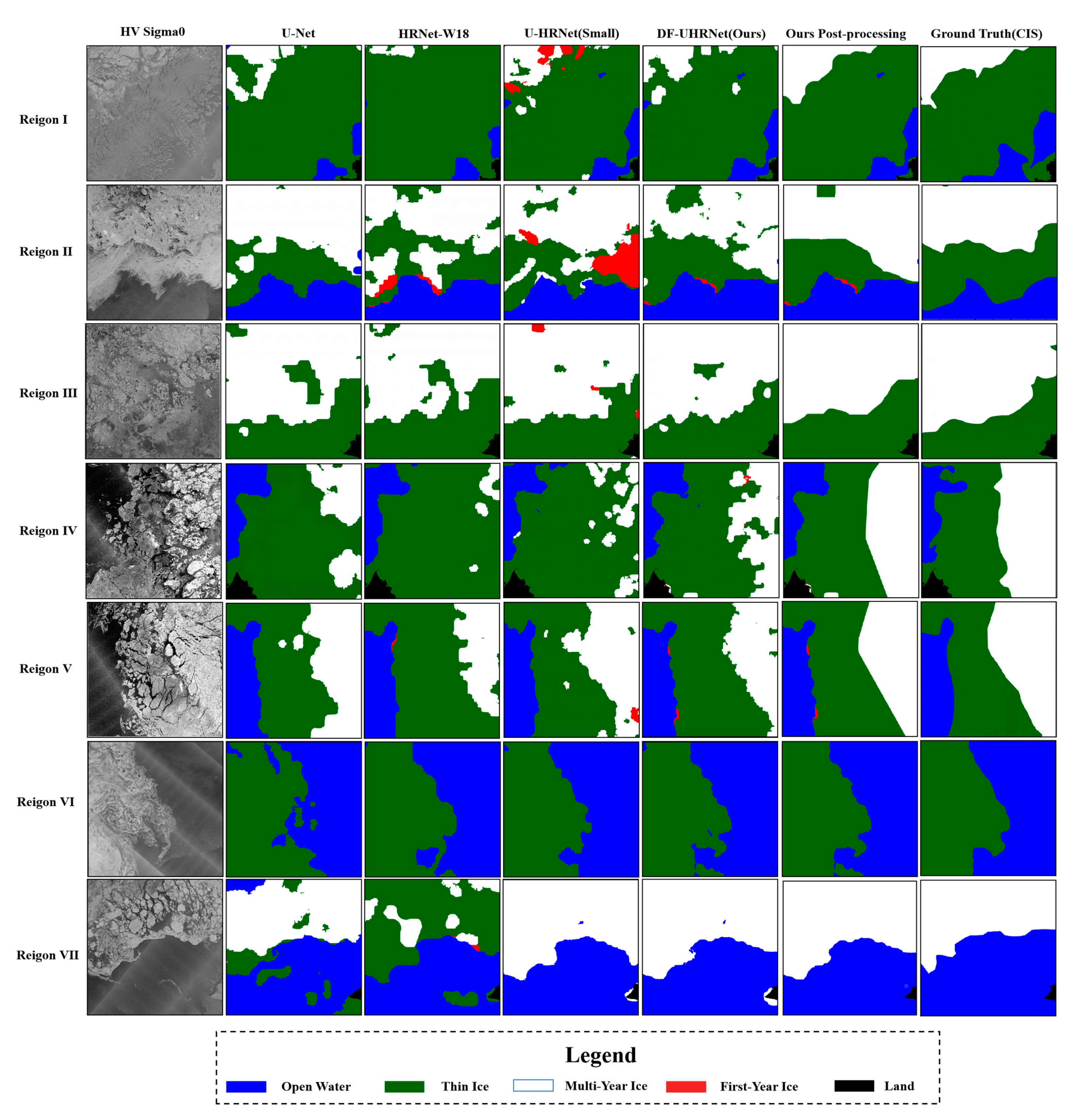
To verify the actual effectiveness of the DF-UHRNet proposed in this study, U-Net, HRNet, and U-HRNet were selected for comparison. Among these, HRNet-W36 and W48 were only selected for comparison with HRNet-W18 because of their poor results in terms of experimental validation. The segmentations and parameter sizes of different models within the same training set can be seen in Figure 12; the data for regions one to five were obtained from the Beaufort Sea, and the sixth and seventh regions, from the Hudson Bay Sea. The detailed parameters can be found in Table 4.
Our network showed good applicability in sea ice segmentation for all seven of the selected regions, and the identification results it yielded were close to those of the CIS ice charts. The original U-HRNet network contains a vast number of parameters, and after improving its fusion module and adding the attention mechanism, the DF-UHRNet network could reach a greater segmentation accuracy by reducing many of its parameters. The overall recognition accuracy was then further improved upon by using the morphological post-processing results. This is because the huge number of parameters prevented the model from achieving further improvements. In this study, by designing a fusion mechanism and reducing the number of convolutional operations enacted by the fusion module, the model’s parameters were optimized. Compared to the UHRNet-Small, the overall quantity of network parameters in the DF-UHRNet was reduced by 20%, while yielding far richer global contextual information, which improved the ability of the network in terms of the extraction and detection of semantic features of sea ice at different scales.
We compared the accuracy indices of our model with those of the four other models. As shown in Table 3, our model achieved the best overall accuracy, MIoU, F1-score, and kappa indices when applied to the recognition task for all five regions; these indices improved by 4.36%, 3.78%, 3.12%, and 7.32% and 2.9%, 3.42%, 3.56%, and 5.96%, compared to the U-Net and U-HRNet (Small), respectively. The regions with identification errors were found to primarily exhibit two categories:
(1) The misclassifications were caused by the similarity of backscattering characteristics among sea ice categories. As shown in region II in Figure 12, the regions of white and gray ice within the multi-year and thin ice areas are more similar in terms of backscattering characteristics, resulting in confusion in identification.
(2) This is due to the coarse granularity of the ice chart itself, as a result of which, although the confused and small areas of sea ice were extracted, they were not marked in the ice chart. Such problems can be effectively solved by using our post-processing algorithm, which preserves the edge details as effectively as possible and corrects the confusion between different sea ice categories.
In addition, our model achieved the fusion of the semantics of adjacent feature scales (no more than two upsampling and downsampling) by regularly adding the fusion module for both scales through its U-shaped structure. As a result, the new semantic features after the fusion module were retained as the feature parts of the adjacent scales (after up- and downsampling), which effectively alleviated the semantic gap problem caused by directly fusing two semantic features with a large-scale gap. From the comparison experiments, the classification model modeled by our method had a significantly higher accuracy. From the actual extraction results in Figure 12, the sea ice types of the seven sea areas involved in the experiment were extracted. Compared with networks such as the U-Net, the DF-UHRNet is more accurate and detailed for the boundary delineation of sea ice types. Its boundary extraction for multi-year ice, thin ice, and open sea ice is more consistent with the actual sea ice category distribution obtained from the visual interpretation compared with the U-Net, HRNet, and UHRNet networks.
The recognition results achieved following the introduction of the post-processing method were closer to those within the original ice map, and the evaluation results improved by 4.64%, 3.54%, 1.57%, and 7.28%, respectively, with an overall recognition accuracy of 90.5% and a kappa coefficient of 81.78%. By comparing the identification results of different regions, we can conclude that our model reveals clear sea ice boundaries, offers more accurate extraction results, and requires fewer network parameters in its deployment compared with the other models. The proposed post-processing method can thus effectively fit the identification results to the original ice chart data.

4. Conclusions

In this study, a fully automated sea ice segmentation process based on deep learning was designed for use in sea ice classification during the Arctic summer ice melt cycle, offering a high-resolution sea ice concentration feature calculation method. The main improvements yielded by our method compared to previous methods are as follows:
(1)
A method is proposed for extracting sea ice concentrations using a K-means++ clustering algorithm and fast convolution operation. Since its extraction is based on SAR images and is fast and accurate in real time, the data can reflect the spatial distribution of sea ice very effectively. Compared with the direct introduction of sea ice concentration products obtained based on radiometric input features, this method not only has higher spatial resolution but also matches the time of SAR features.
(2)
A new fully convolutional neural network DF-UHRNet is proposed, which enables the more effective fusion of high-resolution weak semantic features (focusing on the representation of edges in sea ice) and low-resolution strong semantic features (focusing on the abstract morphology of sea ice) via the design of a dual-scale fusion module. Because a vacuity convolution pyramid module is added to the high-level fusion module, the perceptual field of the convolution kernel can be expanded without any loss of resolution (no feature sampling) and thus, sea ice semantic features can be more effectively extracted. The two fusion modules were carefully designed to facilitate not only the fusion of adjacent scale features, but also to reduce the overall quantity of parameters within the model.
(3)
The method achieves a fully automated sea ice classification with a full process flow. All processes do not require additional human intervention, and the fully convolutional neural network facilitates end-to-end sea ice semantic segmentation. Thus, it contributes to the fully automated mapping of Arctic sea ice.
The DF-UHRNet that we designed, compared with the U-Net, HRNet, and U-HRNet, improves recognition capacity and the number of parameters in the model is optimized, which means that the network has greater portability and extensibility and is more convenient for deployment in projects.
From a practical point of view, our method is also applicable to other sea areas. The most likely limitation relates to the area of coverage of the ice charts and the supporting data. However, we can resolve this by replacing the ice chart data; for example, in the Northeast Passage region of the Arctic, the CIS weekly ice map product can be replaced by replacing other regional ice map products published by AARI to generate the training set. In addition, since the weekly ice charts are released every Monday and the relay period of Sentinel-1A/B is 6 days, although the 2020 data appear sufficient for training, the relay period of Sentinel-1 data actually increases to 12 days given that the Sentinel-1B satellite has been offline since 2022, which may result in a data shortage for the periods after 2022. In terms of extraction time, the present method not only quickly extracts sea ice types in the Arctic region during the melt ice period but can also quickly extract sea ice types other than seasonal ones. However, considering the effect of seasonal freezing cycles in the Arctic, the sea ice category may be relatively homogeneous during winter and spring, when ice concentration is close to 100% due to extensive freezing. Sea ice concentration indicates the spatial distribution of sea ice in the region and therefore is not very meaningful to introduce. Therefore, the sea ice concentration feature can be discarded before carrying out deep learning sea ice classification during winter and spring periods.
In this regard, in addition to training with multi-year data, the introduction of new SAR satellite remote sensing data is also worth considering, since a large number of satellites are currently in service, such as the C-band GF-3 satellite series launched by China in 2016 [36], the C-band Radarsat-2 satellite launched by Canada in 2017 [7], the Russian Arktika-M-1 Arctic weather monitoring satellite [37], etc. In addition, new approaches can be considered, such as cryosphere detection using remote sensing data acquired via GNSS-R technology. This approach offers high temporal and spatial resolution, meaning it has broad application prospects. It can be used as a research object or data supplement and needs to be studied in the future.
In the future, we will seek to use deep semi-supervised learning and unsupervised learning for Arctic sea ice mapping, as this will help to reduce the labor costs associated with sea ice mapping. We will also further refine the sea ice categories to provide more reliable ice data for Arctic navigation.

Author Contributions

Conceptualization, R.H. and C.W.; methodology, R.H. and C.W.; software, R.H.; writing—original draft preparation, R.H. and C.W.; writing—review and editing, J.L. and Y.S.; funding acquisition, C.W. and Y.S. All authors have read and agreed to the published version of the manuscript.

Funding

This work was supported by the National Natural Science Foundation of China (No. 62172247).

Data Availability Statement

Data presented in this study are available upon request from the corresponding author.

Acknowledgments

The authors would like to thank the anonymous reviewers and members of the editorial team for their comments and contributions.

Conflicts of Interest

The authors declare no conflict of interest.

Abbreviations

The following abbreviations are used in this manuscript:
CISCanadian Ice Service
CBAMConvolutional Block Attention Module
CNNConvolutional Neural Network
ResNetResidual Network
CRFConditional Random Field
AARIArctic and Antarctic Research Institute
HRNetHigh-Resolution Network
U-HRNetU-Shaped High-Resolution Network
U-NetU-Shaped Convolutional Network
Grad-CAMGradient-weighted Class Activation Mapping
BDBhattacharyya Distance
SISeparability Index
SICSea Ice Concentration
ASPPAtreus Spatial Pyramid Pooling
SARSynthetic Aperture Radar
HDCHybrid Dilated Convolution
IMOInternational Maritime Organization
PCAPrincipal Component Analysis
EWExtra-Wide Swath
GLCMGray-Level Concurrence Matrix
SVMSupport Vector Machine
FFTFast Fourier Transform

References

  1. Sinha, N.K.; Shokr, M. Sea Ice: Physics and Remote Sensing; John Wiley & Sons: Hoboken, NJ, USA, 2015. [Google Scholar]
  2. Kwok, R. Arctic sea ice thickness, volume, and multiyear ice coverage: Losses and coupled variability (1958–2018). Environ. Res. Lett. 2018, 13, 105005. [Google Scholar] [CrossRef]
  3. Xu, J.; Tang, Z.; Yuan, X.; Nie, Y.; Ma, Z.; Wei, X.; Zhang, J. A VR-based the emergency rescue training system of railway accident. Entertain. Comput. 2018, 27, 23–31. [Google Scholar] [CrossRef]
  4. Ghiasi, S.Y. Application of GNSS Interferometric Reflectometry for Lake Ice Studies. Master’s Thesis, University of Waterloo, Waterloo, ON, Canada, 2020. [Google Scholar]
  5. Ghiasi, Y.; Duguay, C.R.; Murfitt, J.; van der Sanden, J.J.; Thompson, A.; Drouin, H.; Prévost, C. Application of GNSS Interferometric Reflectometry for the Estimation of Lake Ice Thickness. Remote Sens. 2020, 12, 2721. [Google Scholar] [CrossRef]
  6. Yan, Q.; Huang, W. Sea ice sensing from GNSS-R data using convolutional neural networks. IEEE Geosci. Remote Sens. Lett. 2018, 15, 1510–1514. [Google Scholar] [CrossRef]
  7. Liu, H.; Guo, H.; Zhang, L. SVM-based sea ice classification using textural features and concentration from RADARSAT-2 dual-pol ScanSAR data. IEEE J. Sel. Top. Appl. Earth Obs. Remote Sens. 2014, 8, 1601–1613. [Google Scholar] [CrossRef]
  8. Changying, W.; Dezheng, T.; Yuanfeng, H.; Yi, S.; Jialan, C. Sea Ice Classification of Polarimetric SAR Imagery based on Decision Tree Algorithm of Attributes’ Subtraction. Remote Sens. Technol. Appl. 2021, 33, 975–982. [Google Scholar]
  9. Lohse, J.; Doulgeris, A.P.; Dierking, W. An optimal decision-tree design strategy and its application to sea ice classification from SAR imagery. Remote Sens. 2019, 11, 1574. [Google Scholar] [CrossRef]
  10. Zhang, S.; Zhang, J.; Xun, L.; Wang, J.; Zhang, D.; Wu, Z.J.I.G.; Letters, R.S. AMFAN: Adaptive Multiscale Feature Attention Network for Hyperspectral Image Classification. IEEE Geosci. Remote Sens. Lett. 2022, 19, 1–5. [Google Scholar] [CrossRef]
  11. Wang, P.; Chen, P.; Yuan, Y.; Liu, D.; Huang, Z.; Hou, X.; Cottrell, G. Understanding convolution for semantic segmentation. In Proceedings of the 2018 IEEE winter conference on applications of computer vision (WACV), Lake Tahoe, CA, USA, 12–15 March 2018; pp. 1451–1460. [Google Scholar]
  12. De Gelis, I.; Colin, A.; Longépé, N. Prediction of categorized sea ice concentration from Sentinel-1 SAR images based on a fully convolutional network. IEEE J. Sel. Top. Appl. Earth Obs. Remote Sens. 2021, 14, 5831–5841. [Google Scholar] [CrossRef]
  13. Huang, D.; Li, M.; Song, W.; Wang, J. Performance of convolutional neural network and deep belief network in sea ice-water classification using SAR imagery. J. Image Graph. 2018, 23, 1720–1732. [Google Scholar]
  14. Onstott, R.G.; Carsey, F. SAR and scatterometer signatures of sea ice. Microw. Remote Sens. Sea Ice 1992, 68, 73–104. [Google Scholar]
  15. Torres, R.; Snoeij, P.; Geudtner, D.; Bibby, D.; Davidson, M.; Attema, E.; Potin, P.; Rommen, B.; Floury, N.; Brown, M. GMES Sentinel-1 mission. Remote Sens. Environ. 2012, 120, 9–24. [Google Scholar] [CrossRef]
  16. Galley, R.; Key, E.; Barber, D.; Hwang, B.; Ehn, J. Spatial and temporal variability of sea ice in the southern Beaufort Sea and Amundsen Gulf: 1980–2004. J. Geophys. Res. Ocean. 2008, 113. [Google Scholar] [CrossRef]
  17. Shlens, J. A tutorial on principal component analysis. arXiv 2014, arXiv:1404.1100. [Google Scholar]
  18. Chen, L.-C.; Papandreou, G.; Kokkinos, I.; Murphy, K.; Yuille, A.L. Deeplab: Semantic image segmentation with deep convolutional nets, atrous convolution, and fully connected crfs. IEEE Trans. Pattern Anal. Mach. Intell. 2017, 40, 834–848. [Google Scholar] [CrossRef]
  19. Jian, W.; Yubao, Q.; Zhenhua, X.; Xiping, Y.; Jingtian, Z.; Lin, H.; Lijuan, S. Comparison and verification of remote sensing sea ice concentration products for Arctic shipping regions. Chin. J. Polar Res. 2020, 32, 301. [Google Scholar]
  20. Cavalieri, D.; Crawford, J.; Drinkwater, M.; Eppler, D.; Farmer, L.; Jentz, R.; Wackerman. Aircraft active and passive microwave validation of sea ice concentration from the Defense Meteorological Satellite Program Special Sensor Microwave Imager. J. Geophys. Res. Ocean. 1991, 96, 21989–22008. [Google Scholar] [CrossRef]
  21. Arthur, D.; Vassilvitskii, S. k-Means++: The Advantages of Careful Seeding; SODA 2007: New Orleans, LA, USA, 2006. [Google Scholar]
  22. Mundy, C.; Barber, D. On the relationship between spatial patterns of sea-ice type and the mechanisms which create and maintain the North Water (NOW) polynya. Atmosphere-Ocean 2001, 39, 327–341. [Google Scholar] [CrossRef]
  23. Remund, Q.; Long, D.; Drinkwater, M. Polar sea-ice classification using enhanced resolution NSCAT data. In Proceedings of the IGARSS’98. Sensing and Managing the Environment. 1998 IEEE International Geoscience and Remote Sensing. Symposium Proceedings.(Cat. No. 98CH36174), Seattle, WA, USA, 6–10 July 1998; pp. 1976–1978. [Google Scholar]
  24. Zhang, Q.; Skjetne, R.; Løset, S.; Marchenko, A. Digital image processing for sea ice observations in support to Arctic DP operations. In Proceedings of the International Conference on Offshore Mechanics and Arctic Engineering, Rio de Janeiro, Brazil, 1–6 July 2012; pp. 555–561. [Google Scholar]
  25. Aggarwal, S. Satellite Remote Sensing and GIS Applications in Agricultural Meteorology. Princ. Remote Sens. 2004, 23, 23–28. [Google Scholar]
  26. Mathieu, M.; Henaff, M.; LeCun, Y. Fast training of convolutional networks through ffts. arXiv 2013, arXiv:1312.5851. [Google Scholar]
  27. Wang, J.; Long, X.; Chen, G.; Wu, Z.; Chen, Z.; Ding, E. U-HRNet: Delving into Improving Semantic Representation of High Resolution Network for Dense Prediction. arXiv 2022, arXiv:2210.07140. [Google Scholar]
  28. Ronneberger, O.; Fischer, P.; Brox, T. U-net: Convolutional networks for biomedical image segmentation. In Proceedings of the Medical Image Computing and Computer-Assisted Intervention–MICCAI 2015: 18th International Conference, Munich, Germany, 5–9 October 2015; pp. 234–241. [Google Scholar]
  29. Wang, J.; Sun, K.; Cheng, T.; Jiang, B.; Deng, C.; Zhao, Y.; Liu, D.; Mu, Y.; Tan, M.; Wang, X. Deep high-resolution representation learning for visual recognition. IEEE Trans. Pattern Anal. Mach. Intell. 2020, 43, 3349–3364. [Google Scholar] [CrossRef] [PubMed]
  30. Woo, S.; Park, J.; Lee, J.-Y.; Kweon, I.S. Cbam: Convolutional block attention module. In Proceedings of the European conference on computer vision (ECCV), Munich, Germany, 8–14 September 2018; pp. 3–19. [Google Scholar]
  31. Chen, L.-C.; Zhu, Y.; Papandreou, G.; Schroff, F.; Adam, H. Encoder-decoder with atrous separable convolution for semantic image segmentation. In Proceedings of the European conference on computer vision (ECCV), Munich, Germany, 8–14 September 2018; pp. 801–818. [Google Scholar]
  32. Fukunaga, K. Introduction to Statistical Pattern Recognition; Elsevier: Amsterdam, The Netherlands, 2013. [Google Scholar]
  33. Cumnling, I.; van Zyl, J. Feature Utility In Polarimetric Radar Image Classificatiion. In Proceedings of the 12th Canadian Symposium on Remote Sensing Geoscience and Remote Sensing Symposium, 10–14 July 1989; pp. 1841–1846. [Google Scholar]
  34. Haralick, R.M.; Shanmugam, K.; Dinstein. Textural features for image classification. IEEE Trans. Syst. Man Cybern. 1973, SMC-3, 610–621. [Google Scholar] [CrossRef]
  35. Selvaraju, R.R.; Cogswell, M.; Das, A.; Vedantam, R.; Parikh, D.; Batra, D. Grad-cam: Visual explanations from deep networks via gradient-based localization. In Proceedings of the IEEE International Conference On Computer Vision, Venice, Italy, 22–29 October 2017; pp. 618–626. [Google Scholar]
  36. Zhang, L.; Liu, H.; Gu, X.; Guo, H.; Chen, J.; Liu, G. Sea ice classification using TerraSAR-X ScanSAR data with removal of scalloping and interscan banding. IEEE J. Sel. Top. Appl. Earth Obs. Remote Sens. 2019, 12, 589–598. [Google Scholar] [CrossRef]
  37. Asmus, V.; Milekhin, O.; Kramareva, L.; Khailov, M.; Shirshakov, A.; Shumakov, I. Arktika-M: The world’s first highly elliptical orbit hydrometeorological space system. Russ. Meteorol. Hydrol. 2021, 46, 805–816. [Google Scholar] [CrossRef]
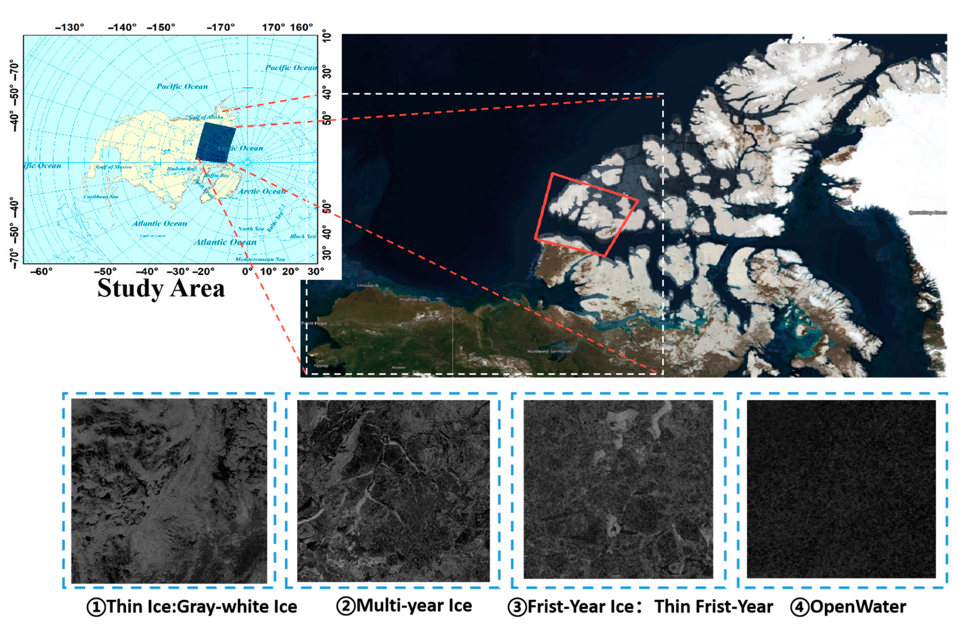
Figure 1. The study area and the typical sea ice types covered in summer in this area, in the form of the type of sea ice development stage.
Remotesensing 15 02448 g001
Figure 2. Overall process of automatic extraction of sea ice classification information.
Remotesensing 15 02448 g002
Figure 3. Results of high-resolution sea ice concentration extraction and related processes. (a) Open water area extraction based on the deep learning method; (b) ice water map extracted based on the K-means++ algorithm; (c) the calculated high-resolution sea ice concentration; and (d) the results after dimension reduction by PCA.
Remotesensing 15 02448 g003
Figure 4. The ice-water segmentation results extracted by different algorithms and the final extracted sea ice concentration value.
Remotesensing 15 02448 g004
Figure 5. Overall structure of the DF-UHRNet network.
Remotesensing 15 02448 g005
Figure 6. Convolutional Block Attention Module (CBAM).
Remotesensing 15 02448 g006
Figure 7. Architecture of the high-level fusion module and low-level fusion module.
Remotesensing 15 02448 g007
Figure 8. The overall process of post-processing based on morphological methods.
Remotesensing 15 02448 g008
Figure 9. The optimal texture feature extraction window found based on the Bhattacharyya distance (BD) and separability index (SI). (a) HV texture separability calculated using the BD index; (b) HV texture separability calculated using the SI index; (c) HH texture separability calculated using the BD index; and (d) HH texture separability calculated using the SI index.
Remotesensing 15 02448 g009
Figure 10. Feature optimization operation based on the Bhattacharyya distance and separability index.
Remotesensing 15 02448 g010
Figure 11. The class activation graph output using the Grad-CAM algorithm. The feature visualization between different models is presented horizontally and the feature visualization of different sea ice extraction tasks is presented vertically.
Remotesensing 15 02448 g011
Figure 12. Comparison of sea ice classification results of the U-Net, HRNet, UHRNet, and DF-UHRNet in five different regions.
Remotesensing 15 02448 g012
Table 1. Results obtained from feature optimization based on the Bhattacharyya distance and separability index for 26-dimensional features.
Feature NameSIBDFeature NameSIBD
σ H H 0 0.188550.05806 H H m a 0.011550.03611
σ H v 0 0.147730.42784 H H e n t 0.023390.02824
σ H H 0 + σ H v 0 0.039510.01751 H H e n e 0.019250.00186
σ H H 0 σ H v 0 0.088920.32102 H V m e a n 0.207750.01695
σ H H 0 / σ H v 0 0.088840.31103 H V s t d 0.055960.49085
( σ H H 0 σ H v 0 ) / σ H H 0 + σ H v 0 0.039610.03763 H V m e a n 0.021760.18168
( σ H v 0 σ H H 0 ) / σ H H 0 + σ H v 0 0.039650.01751 H V c o n t 0.018940.14584
H H m e a n  10.078680.20947 H V d i s s 0.014360.16384
H H s t d 0.042510.08298 H V h o m o 0.030690.16254
H H c o n t 0.025370.05249 H V m a 0.019540.24148
H H d i s s 0.024590.04681 H V a s m 0.035350.19041
H H h o m o 0.020070.03159 H V e n t 0.031050.25662
H H a s m 0.018960.03611 H V e n e 0.011550.24384
1 where the subscripts of HH and HV features in mean, std, cont, diss, homo, asm, ma, ent, ene represent the mean, standard deviation, contrast, homogeneity, dissimilarity, angular second moment, energy, and entropy in the grayscale coeval matrix of the corresponding feature calculation, respectively.
Table 2. Number of data slices for each category in open ocean extraction and sea ice classification for deep learning tasks.
MethodCategory NameOriginal SamplesAugmented SamplesFinal Samples
Open Water SegmentationOpen Water169043106000
Sea Ice17,20406000
Sea Ice ClassificationMulti-year Ice13,78004000
One-year Ice238816124000
Thin Ice102929714000
Table 3. Comparison of ablation experiment precision values.
ModelParametersOA (%)MIoU (%)
HRNet-W189,671,83582.572.8
DF-UHRNet (L_1, H_2/without ASPP) 16,128,39182.573.6
DF-UHRNet (without CBAM)5,077,41191.585.3
DF-UHRNet (without CRF)5,079,17587.479.4
DF-UHRNet (without SIC)5,079,17588.781.7
Our Model5,079,17591.686.5
1 where DF-UHRNet (L in L_1 indicates that the number of convolutional modules of the low-level fusion module is 1 and H_2 indicates that the number of convolutional modules of the high-level fusion module is 2). Alternatively, we also used a model that lacked the Atreus Pyramid Convolution Module.
Table 4. Results of the evaluation of four networks and post-processing in five regions after introducing high-resolution sea ice concentration features.
MethodParams 1Model Size (MB) 2MIoU (%)Accuracy (%)F1 (%)Kappa (%)
HRNet-W189,671,835118.21267.6077.0276.9555.12
U-Net10,158,707119.57174.1483.1883.4367.18
U-HRNet (Small)6,107,10772.96675.6083.5482.9968.54
DF-UHRNet (Ours)5,079,17561.24878.5086.9686.5574.50
Our Post-processing5,079,17561.24883.1490.5088.1281.78
1 “Params” is the total number of parameters to be trained during model training. 2 “Model Size” is the storage space occupied by the model.
Disclaimer/Publisher’s Note: The statements, opinions and data contained in all publications are solely those of the individual author(s) and contributor(s) and not of MDPI and/or the editor(s). MDPI and/or the editor(s) disclaim responsibility for any injury to people or property resulting from any ideas, methods, instructions or products referred to in the content.