Faint Echo Extraction from ALB Waveforms Using a Point Cloud Semantic Segmentation Model

Abstract

As an active remote sensing technology, airborne LIDAR can work at all times while emitting specific wavelengths of laser light that can penetrate seawater. Airborne LIDAR bathymetry (ALB) records an object’s full return waveform, including the water surface, water column, seafloor, and the objects on it. Due to the seawater’s absorption and scattering and the seafloor’s reflectivity effect, the seafloor’s amplitude of seafloor echoes varies greatly. Seafloor echoes with low signal-to-noise ratios are not easily detected using waveform processing methods, which can lead to insufficient seafloor topography depth and incomplete seafloor topography coverage. To extract faint seafloor echoes, we proposed a depth extraction method based on the PointConv deep learning model, called FWConv. The method assumed that spatially adjacent echoes were correlated. We converted all the spatially adjacent multi-frame waveforms into a point cloud. Each point represented a bin value in the waveform, and the points’ properties contained spatial coordinates and the amplitude in the waveform. In the semantic segmentation of these point clouds using deep learning models, we considered not only each centroid’s amplitude, but also its neighboring points’ distance and amplitude. This enriched the centroids’ features and allowed the model to better discriminate between background noise and seafloor echoes. The results showed that FWConv could extract faint seafloor echoes in the experimental area and was not easily affected by noise, and that the correctness reached 99.82%. The number of point clouds increased by 158%, and the seafloor elevation accuracy reached 0.20 m concerning the multibeam echo sounder data.

1. Introduction

Airborne LIDAR bathymetry (ALB) emits a laser with high-frequency and high-pulse energy within the wavelength in the seawater transmittance window and records an echo’s full waveform. The echo moments of the sea surface and seafloor are extracted from the recorded waveform and combined with the inertial measurement unit (IMU) and global positioning system (GPS) information to solve the seafloor’s geodetic position. ALB can be efficient and safe for completing high-precision three-dimensional seafloor topographic mapping compared to sonar-based shipboard mapping. The laser transmission process includes refraction and reflection from the sea–air interface, absorption and scattering from seawater, and reflection from the seafloor substrate. The pulse energy decays exponentially with the transmission depth and the decay rate is positively correlated with the water column’s turbidity, which may result in low signal-to-noise ratio seafloor echoes. These low signal-to-noise ratio seafloor echoes can also be created when the seafloor’s reflectivity substrate is weak.

To improve seafloor echo detection in low signal-to-noise ratio waveforms, waveform processing methods can be divided into two categories: waveform denoising and waveform estimation or enhancement. Saylam et al. [1] used a moving average filtering algorithm to smooth the waveform. Wang et al. [2] compared some waveform processing methods and concluded that the Richardson–Lucy deconvolution (RLD) [3] method can over-solve the waveform extraction of very shallow water and faint echo signals better, while the average square difference function (ASDF) [4] can handle noise better. However, these methods do not work well when the signal and noise level ratios are very close. There are two reasons for this: (1) if the seafloor echo signal’s amplitude itself is close to the noise level, the method filters the signal out together; and (2) since the echo signal extraction is usually a peak detection method using a fixed threshold, if the filtered signal amplitude is still below the threshold, then the seafloor echo signal is still not detected.

Faint seafloor echoes in a single waveform analysis are barely or not distinguishable from noise, and the reliable detection of these faint seafloor echoes requires much more information. Based on the continuity of the seafloor topography, spatially adjacent waveforms are correlated, so adjacent waveform data of the target waveform can be used for waveform stacking to enhance the seafloor echo signal-to-noise ratio, or for estimating the seafloor echo positions. Kogut et al. [5] achieved good results by estimating the second echo position of only one echo waveform detected using a neighborhood waveform with multiple echoes. However, for waveforms with too high noise or too small echo energy, a second echo position cannot be extracted because it does not satisfy the Gaussian decomposition condition. Yao and Stilla [6] introduced a waveform stacking technique to improve the signal-to-noise ratio of objects within a specific window range. The experimental results showed that, for terrestrial lidar systems (TLSs), the weak reflected signals from partially occluded surfaces could be successfully detected. However, the method is designed for fixed static terrestrial lidar systems. Mader et al. [7] argued that the final water bottom point should not be derived from the stacked full waveform itself, as this results in an undesired smoothing effect (similar to low-pass filtering) and a reduction in the bottom-point resolution.

Some studies have been conducted to classify the waveform data and point clouds obtained using ALB with deep learning models. Zhao et al. [8] proposed a multi-source CNN model to classify the raw waveform data into three categories: land, shallow water, and deep water, with a 99.5% accuracy. Kogut and Slowik [9] used multilayer perceptron neural networks to classify the generated point clouds with 100% for the surface and seafloor point clouds and 80% for the underwater targets. Roshandel et al. [10] used a deep learning model to classify the surface and seafloor point clouds for large scenes. Despite deep learning models’ high accuracy for the classification problem, there is no study on using deep learning methods for the bathymetric extraction of waveform data from ALBs.

Due to waveform processing methods’ limitations and deep learning’s superiority for classification, we propose a method for extracting seafloor echo signals based on PointConv, a deep learning model for the semantic segmentation of point clouds. We call this model for the semantic segmentation of seawater and the sea surface FWConv. FWConv simultaneously processes multiple spatially adjacent waveforms. Each bin value in a waveform is converted to a point within a point cloud, where the point’s features include the spatial coordinates and the waveform’s amplitude, and a sample point contains multiple spatially contiguous waveforms. FWConv extracts each point’s features based on its neighbors, replacing the waveform stacking process. Then, the model semantically segments each point into one of the categories of the surface, seafloor, and background based on each point’s features, which can be approximated as the detection process in waveform processing. The field data from the ALB system are used to evaluate the seafloor echo detection capability and the bottom location’s accuracy. In the next section, a brief introduction to the experimental data and experimental area used in the study is presented, Section 3 describes the method’s implementation process, Section 4 compares the FWConv’s semantic segmentation results with the waveform processing results, Section 5 provides a discussion of the results, and Section 6 presents the conclusions.

2. The Mapper4000U and Study Area

2.1. Mapper4000U

The ocean lidar equipment used to collect the data was the Mapper 4000U, developed by the Shanghai Institute of Optical Precision Machinery, Chinese Academy of Sciences. It is a lightweight and compact marine lidar specifically developed for UAV platforms. It can operate at altitudes of 5–200 m and its data acquisition method is full waveform acquisition. The Mapper4000U’s laser can emit a 1064 nm laser output at a base frequency of 4 KHz with a pulse width of 1–a2ns and achieve a 532 nm laser output after frequency doubling. A rotating scanner is used to create an elliptical scanning pattern with a scan angle of ±15° along the track and about a ±12° cross-track [11].

The sensor consists of two receiver channels: an avalanche photodiode (APD) channel for near-infrared pulses and a photomultiplier tube (PMT) channel for green pulses. The PMT has a wide effective response range to avoid signal saturation in very shallow waters and to ensure a penetration capability of more than 1.5 Secchi Depths (SD). The sampling rate for all the channels is 1 G samples/s, corresponding to a laser transmission distance of approximately 0.15 m in air and 0.11 m in water. Its appearance is shown in Figure 1.

Table 1. Parameters of Mapper4000U.

Parameter	Mapper4000U
Laser re-frequency	4 kHz
Pulse energy	12 uJ@1064 nm 24 uJ@532 nm
Laser pulse width	1.5 ns
Weight	4.4 kg
Scan mode	Elliptical scanning
Scan rate	900 rpm
Size	235 mm × 184 mm × 148 mm

shows its specific parameters.

2.2. Study Area

The experimental area was located on Dazhou Island, Wanning City, Hainan Province, China. The experimental strip’s underwater topography is a continuous gentle slope, suitable for evaluating the system’s bathymetric performance with an SD of 5–10 m. We conducted a flight experiment for the Mapper4000U on Dazhou Island on 26 September 2021 and a ship measurement multibeam verification experiment on September 29. The ship measurement multibeam echo sounder (MBES) used was a Hydro-Tech MS400U. Its specific parameters are listed in

Table 2. Parameters of Hydro-Tech MS400U.

Parameter	Hydro-Tech MS400U
Working Frequency	400 kHz
Depth Resolution	0.75 cm
No. of Beams	512
Working Modes	Equiangular or Equidistance
Vertical Receiving Beam Width	1°
Parallel Transmitting Beam Width	2°
Sounding Range	0.2–150 m

. The flight experiment was intended to test the Mapper4000U’s maximum water depth detection capability, so the UAV landing and takeoff position was the bow-shaped beach between the two ridges of Dazhou Island, and the flight track was a straight line away from the mainland. The UAV’s flight speed in the experiment was 5 m/s with about a 50 m flight height and the total flight time was about 8 min due to the UAV’s battery power. The longitudinal sea distance was about 1100 m and the average point density of the seafloor was 30 points/m². Figure 2 shows the study area.

3. Method

3.1. Workflow

Since the wavelength corresponding to the APD channel was 1064 nm, which cannot penetrate seawater, the data selected for the experiment were from the PMT channel corresponding to 532 nm. The workflow for extracting the echo signals from the ALB waveforms using FWConv is shown in Figure 3.

The first step was constructing training samples for the FWConv model, which required transforming each bin value in the multiple spatially adjacent waveform data into points and labeling each point. Then, the second step was to train the FWConv model using the training set. After training the model, the waveform data to be processed were also converted into point cloud data, and the point cloud semantic segmentation was performed using the FWConv model. The resulting point clouds, labeled as sea surface and seafloor, were retained. When converting the waveform data into training sample point clouds, we did not know which were the sea surface echo moments, so the seawater refraction process was not considered when solving the point clouds. Therefore, the fourth step required was to invert the point cloud results into slope distance information based on semantic segmentation. Finally, the point cloud solving software was used to complete the point cloud solving, considering the seawater refraction for obtaining the point clouds of the sea surface and seafloor. The next few subsections explain each step of the process in more detail.

3.2. Construction of Training Samples

There were two main steps in constructing the training samples: the semantic labeling of the points and selecting the spatial neighborhood waveforms.

3.2.1. Semantic Labeling of Points

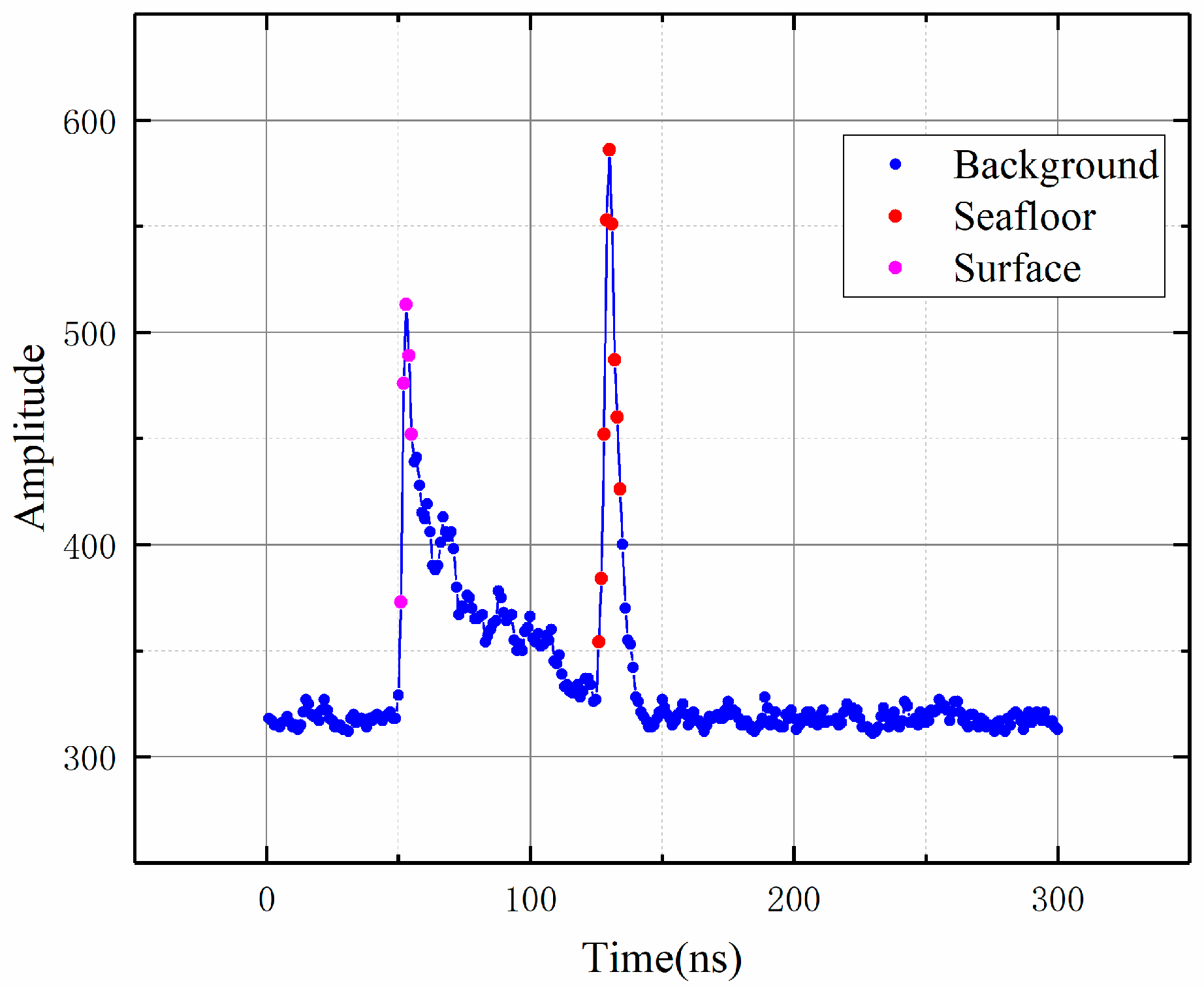
The semantic labeling of the points involved classifying each bin value in the waveform. For each bin value in the waveform, we classified it and then solved it to the sample point cloud. All the waveforms required for the training samples in the experiments were acquired by the Mapper4000U in the experimental area of Figure 2, or obtained by fitting the acquired waveforms. Each bin value in the waveform could be labeled as surface, seafloor, or background. We used the peak detection method to detect the seafloor echo and surface echo in the waveform. For the waveforms that could be detected by performing seafloor echo peak detection, we called them strong seafloor echo waveforms. The echo moment was used as the center for expansion, i.e., the moment of the surface echo and the two points before and after it were labeled as surface points, the moment of the seafloor echo and the four points before and after it were labeled as seafloor points, and the rest of the points were labeled as background points. The extension’s purpose was to avoid a severe imbalance in each category’s number of points. The waveforms within 1 s were selected from the strong echo waveform data every 10 s according to the flight time sequence of the UAV as the waveforms required for the strong echo training samples. A total of about 9 s of waveforms were included and the total number of waveforms was 35,112, covering the water depth range of 2–12 m. The typical waveform bin labeling results are shown in Figure 4.

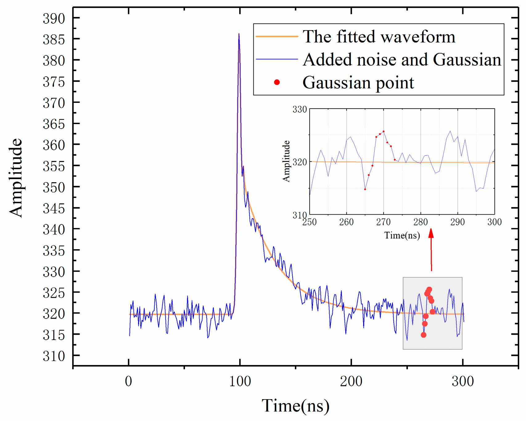
To improve the FWConv model’s semantic segmentation capability for faint seafloor echoes, well-labeled faint seafloor echo waveforms are required. However, the peak detection algorithm fails for faint seafloor echo waveforms, so a method is proposed that uses waveform fitting to construct waveform data without seafloor echoes, and then artificially adds Gaussian functions at specified locations to simulate faint seafloor echo waveforms. Since the added seafloor echo location was artificially provided, the simulated faint seafloor echo waveform could be labeled.

Some studies have been conducted to fit ocean full waveform data, through methods such as using a double Gaussian function [12] or a combination of a trigonometric function and a Weber function [13]. Here, we did not fit the bottom echo part because we artificially added the bottom echo. Since the emitted laser energy was a Gaussian function in the time domain, we simply chose a Gaussian function to fit the sea surface echo. After the laser penetrated the seawater due to the absorption and scattering of the seawater, the returned energy decayed exponentially with distance, so an exponential function was used to fit the energy returned by the seawater. The fitted model $F_w\left(t\right)$ can be expressed as follows:

$$F_w\left(t\right)=f_s\left(t\right)+f_c\left(t\right)$$

(1)

where $f_s\left(t\right)$ is a Gaussian function representing the sea surface return and $f_c\left(t\right)$ is an exponential function representing the scattered part of the seawater. The specific expressions are:

$$f_s\left(t\right)=a\exp \left(-\frac{{\left(t-\mu \right)}^2}{{\delta }^2}\right)$$

(2)

$$f_c(t)=\{\begin{array}{cc}\exp \left(gn+h\right)\left(\frac{t-m}{m-n}\right)& m<t\le n\\ \exp \left(gt+h\right)& n<t\end{array}$$

(3)

where $a$ is the amplitude scaling factor, $\mu$ is the time shift factor, $\delta$ is the time scaling factor, m and n are the horizontal coordinates of the boundary points, and g and h are coefficients related to the seawater scattering. The initial values were selected as described in the article [14] and the parameters were chosen to be optimized using the Levenberg–Marquardt (LM) algorithm.

Furthermore, noise needs to be added to the fitted waveform, which can contain both background and random noise [15]. Background noise is long-term low-frequency noise, which is mainly related to background solar radiation and detector dark currents. Random noise is short-term high-frequency noise, which is mainly caused by random fluctuations inherent to the measurement, and is generally considered to be Gaussian function noise. In this study, the background noise’s effect was ignored and only the Gaussian noise’s effect was considered. The last 50 bin values of the original waveform were counted, their standard deviation was calculated, and the mean value was considered as 0. The Gaussian noise was added according to the calculated standard deviation and mean value.

Finally, a Gaussian function was added at a specific location to simulate the seafloor echo, with a Gaussian function pulse width of 3 ns. The seafloor echo amplitude often jittered within a specific range, while the threshold for the waveform processing methods to discriminate between the echoes was often three times the noise level. This meant that the echo would not be detected when the seafloor echo was smaller than the threshold value. Therefore, to detect more faint echoes, the Gaussian function’s amplitude was three times lower than the noise level, and the following equation determines the amplitude:

$$Amp=Rand\ast 2\ast \delta +1$$

(4)

in which $Rand$ is a random function from 0 to 1 and $\delta$ is the standard deviation of the added Gaussian noise. In the waveform recorded in this flight experiment, the standard deviation of the noise was about 2, so the constructed Gaussian function’s range of amplitude was from about 0.5 times to 2 times $\delta$. According to [16], a method to evaluate the signal-to-noise ratio of the waveforms was proposed:

$$SNR=10lo{g}_{10}{(I}_{seafloor}/\delta )$$

(5)

where $I_{seafloor}$ is the maximum amplitude of the seafloor echo. For the artificially added faint seafloor echoes, $I_{seafloor}$ is the amplitude $Amp$ of the added Gaussian function. Therefore, the $SNR$ of the added faint echo signal ranged from −3 db to 4 db. Since the Gaussian function additions’ locations were manually specified, we could label the weak Gaussian echoes’ bin values. The final constructed faint echo waveform is shown in Figure 5. In total, we generated 21,483 weak echo waveforms and 14,322 waveforms that only fit the surface and water scattering without adding seafloor echoes.

3.2.2. Convert Waveform to Point Cloud

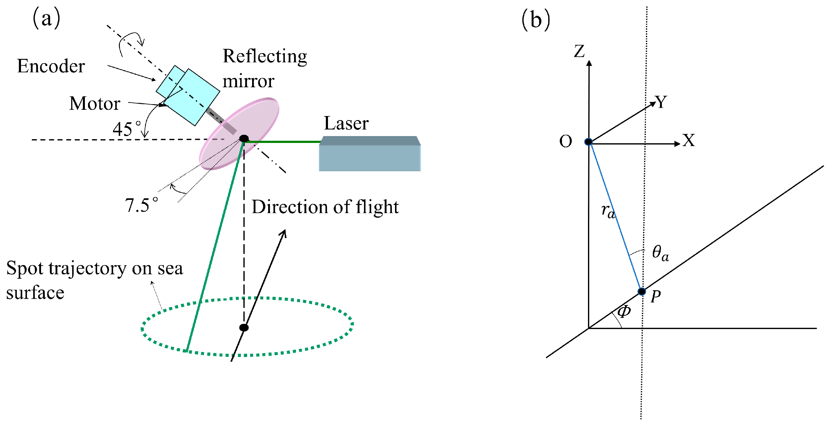
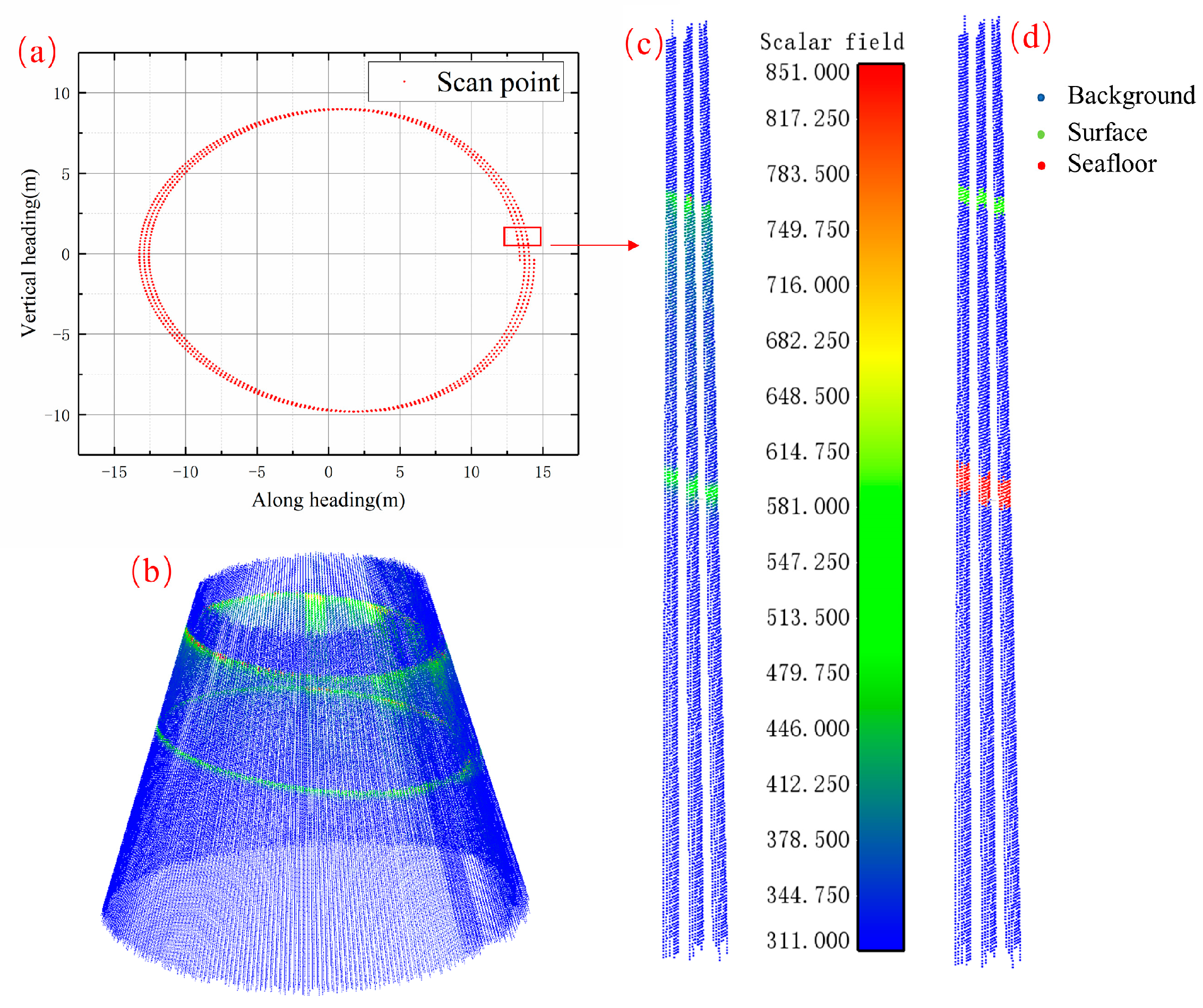
As shown in Figure 6a, a motor-driven reflector was integrated into the Mapper4000U scanning module. The rotation axis of the reflecting mirror and the laser emission direction were at an angle of 45°. The angle between the reflecting mirror’s normal direction and the rotation axis was 7.5°. Therefore, when the motor rotated, the scan trajectory of the Mapper4000U was elliptical, as seen in Figure 7a.

The point $O$ in Figure 6b represents the lidar position when the laser was emitted. The Mapper4000U has a built-in GPS and IMU, so, based on the GPS and internal clock of the lidar, we could know position $O$ when the lidar emitted a laser beam and the initial moment $t_0$ of the laser. A right-handed coordinate system was set up with the origin $O$. The flight direction was the positive direction of the $Y$ axis and the vertical upward direction was the positive direction of the $Z$ axis. The emitted laser’s direction could be determined from the IMU and the encoder value of the motor, including the angle ${\theta }_a$ between the laser and the $Z$ axis, and the angle $\varphi$ between the emitted laser’s projection direction in the $XY$ plane and the positive direction of the $X$ axis. Thus, for any moment $t$ in the waveform, the conversion to point $P$ can be expressed as:

$$P\left(t\right)=O+r_a\left(t\right)$$

$$r_a\left(t\right)=L\left(t\right){\gamma }_a=\frac{c_a\left(t-t_0\right)}{2}{\gamma }_a$$

(6)

$${\gamma }_a={(sin{\theta }_{a}cos\varphi ,sin{\theta }_{a}sin\varphi ,cos{\theta }_a)}^T$$

where $r_a$ is the laser ray equal to the transmission distance $L$ multiplied by the unit vector ${\gamma }_a$, and $c_a$ is the speed of light in air. We converted all the moments in the waveform into points, and the properties of each point included the spatial coordinates and amplitude in the waveform.

3.2.3. Selection of Spatial Neighborhood Waveforms

As seen from the constructed faint echo waveforms, the faint seafloor echoes within a single waveform are almost indistinguishable from the noise. To provide more information to the echo waveforms, we converted multiple spatially neighboring waveforms into a point cloud for the semantic segmentation. Based on the seafloor topography’s continuity, even if the seafloor echoes were weak, the spatially adjacent seafloor echoes of multiple waveforms were concentrated at specific locations in the geometric space. Therefore, converting the spatially neighboring multiple waveforms into a point cloud could provide more information for the semantic segmentation of the echoes.

The Mapper4000U records a laser echo length of 600 ns, of which the atmospheric portion above the sea surface is about 50 ns in duration. From the MBES measurements, the water depth range in the experimental area was less than 20 m, which is about 180 ns. Therefore, the echoes acquired after 230 ns could be considered as background noise. Considering the model training and memory consumption efficiency during the training, a sample contained 21 waveforms and each waveform needed to remove the useless parts. To exclude the ups and downs of the UAV flight altitude, the last 300 ns of the waveform were selected for discarding, so the length of each waveform was fixed to 300 and each sample contained a total of 6300 original waveform points. Each point contained four features: X, Y, Z, and the waveform amplitude. To ensure that the waveforms in the sample were all neighboring in space, the waveforms were selected based on the laser scanning method and the laser flight direction. Specifically, a sample contained 21 consecutive waveforms in the same angular range on three ellipses continuously scanned using the LiDAR, corresponding to the 7 waveforms contained in each ellipse’s angular range. In the experiment, the scanning mirror rotation speed of the Mapper4000U was 900 rpm and the laser re-frequency was 4 KHz, so the number of laser scanning pulses was about 270 during one rotation. Thus, the scan data of one lap could be divided into 38 different groups of scan angle ranges by seven waveforms. According to the UAV’s flight height and speed, the distance between the different frames’ points was about 0.3 m and the distance between the same frames waqs 0.15 m. Due to the different scanning angles, the samples’ neighboring frames corresponding to the different angle ranges were arranged differently; the specific sample examples can be seen in Figure 7. Since one sample contained 21 echo waveforms, 1672 strong echo training samples were constructed based on the strong echo waveforms. Similarly, the number of weak echo training samples was 1023 and the number of no echo waveform training samples was 682.

3.3. FWConv

3.3.1. PointConv and Problem Statement

The typical neural network methods for classifying and segmenting images cannot be directly applied to point clouds due to their data structure’s irregular nature. In a pioneering work, PointNet adopted point clouds as its input and overcame the effect of the unordered point cloud data using symmetric functions [17]. The shortcoming of PointNet is that it calculates each point’s features without considering the neighboring points’ features. Therefore, Qi et al. [18] proposed a hierarchical network, PointNet++, to extract the features from each point’s neighborhood. PointNet++ extracts neighborhood features based on the local point-based PointNet learning layer, while the PointNet learning layer finally expresses a point’s local features only using max pooling, so that only the most obvious local or global feature information can be retained, whereas the other relatively non-obvious information is directly discarded. To extract better and express local features, Wu et al. [19] proposed a convolution operation that extended traditional image convolution into the point cloud called PointConv. The PointConv convolution kernel is considered a nonlinear function of a 3D point’s local coordinates, consisting of a weight function. For a given point, the weight function is learned through a multilayer perceptron network. Figure 8 shows PointConv’s process in a local area centered on a point $\left(p0,f0\right)$. The $k$ neighborhood point features of $p_0$ are extracted to the feature length of $C_{out}$ using PointConv.

Our network input’s points contain geometric information and the waveform amplitude. An input point cloud corresponds to one of the samples above and contains 21 spatially adjacent waveform points in the form of an $N\times C$ matrix. N is the number of waveform points and C is each point’s feature length, consisting of spatial information (X, Y, and Z) and the waveform amplitude. We aim to teach the network to predict the probability that a point in each input belongs to a particular class, as shown in Figure 9. Here, M is the number of classes (surface, seafloor, and background).

3.3.2. Semantic Segmentation Architecture

In this section, we present FWConv’s architecture for semantic segmentation. Figure 10 shows an overview of the FWConv architecture. FWConv’s feature propagation process can be divided into feature encoding and feature decoding. The whole network connects three layers of the feature encoding layer and three layers of the feature decoding layer for its feature propagation.

In the feature encoding layer, the $n_1$ points with a feature vector length $c_1$ are inputs, and $n_2$ points are then randomly sampled from the $n_1$ points. For each point in $n_2$ and its neighbors, the features of length $c_2$ are extracted using PointConv. With each pass of the set feature encoding, the point cloud is downsampled, and the point feature vector corresponds to a larger perceptual field of view.

The downsampled point cloud features need to be propagated back to the original point cloud, which is called feature decoding. The feature decoding process consists of two processes, interpolation and PointConv. The interpolation process involves finding the three nearest neighbor points from the downsampled point cloud centered on the denser point cloud coordinates and interpolating the feature vectors of these three points to the denser point cloud coordinates, by assigning different weights according to the distance. As shown in Figure 10, the $n_4$ points with a feature vector $c_4$ are interpolated to generate $n_3$ points with a feature vector $c_4$. The $n_3$ points with the feature vector $c_3$ are combined with the $c_4$ feature vectors in the feature extraction process to obtain a feature vector of the length $\left(c_3+c_4\right)$. After one more PointConv, the feature vector length is converted to $c_5$ to complete the feature decoding process. The feature decoding process is carried out through several layers until the point cloud is upsampled to the original point cloud.

Finally, the feature vector $c_7$ is connected to the multilayer perceptron. After the transformation in the multilayer perceptron layer, each point’s class probability is estimated by the softmax layer:

$$p_i=\frac{e^{y^i}}{{\sum }_{k=1}^M{e}^{y^k}}$$

(7)

where $p_i$ is the probability that a point belongs to class $i$, $y^i$ is the value of each class output by the multilayer perceptron, and $M$ is the total number of classes.

In the optimization process, we need to minimize the loss function to minimize the difference between the actual value and the FWConv’s predicted value. Since the weak seafloor class is more complicated than extracting than other classes, we use the Focal Loss function [20], which allows the model to focus more on the hard-to-classify samples during training. The Focal Loss function is defined as:

$$L_{FL}=-{\displaystyle \sum _{i=1}^N}{\displaystyle \sum _{j=1}^M}{\left(1-y_{i,j}\right)}^{\gamma }{H}_{i,j}log\left(y_{i,j}\right)$$

(8)

where $y_{i,j}$ is the probability that point $i$ belongs to class $j$, $H_{i,j}$ is the ground truth in class j as a one-hot representation, and ${\left(1-y_{i,j}\right)}^{\gamma }$ is called the modulating factor. When the $y_{i,j}$ is small, the adjustment factor is close to 1 and the loss function is unaffected, while when the $y_{i,j}$ is close to 1, the adjustment factor is close to 0, which reduces the contribution of the better-classified points to the loss function.

The data preprocessing included point cloud coordinate centering and point cloud coordinate normalization, and the model was trained for 100 epochs. The model that achieved the best Mean Intersection over Union (MIoU) on the validation set was selected as the final model, with an MIoU value of 87.1%.

3.4. Obtain Slope Distance from the Point Cloud

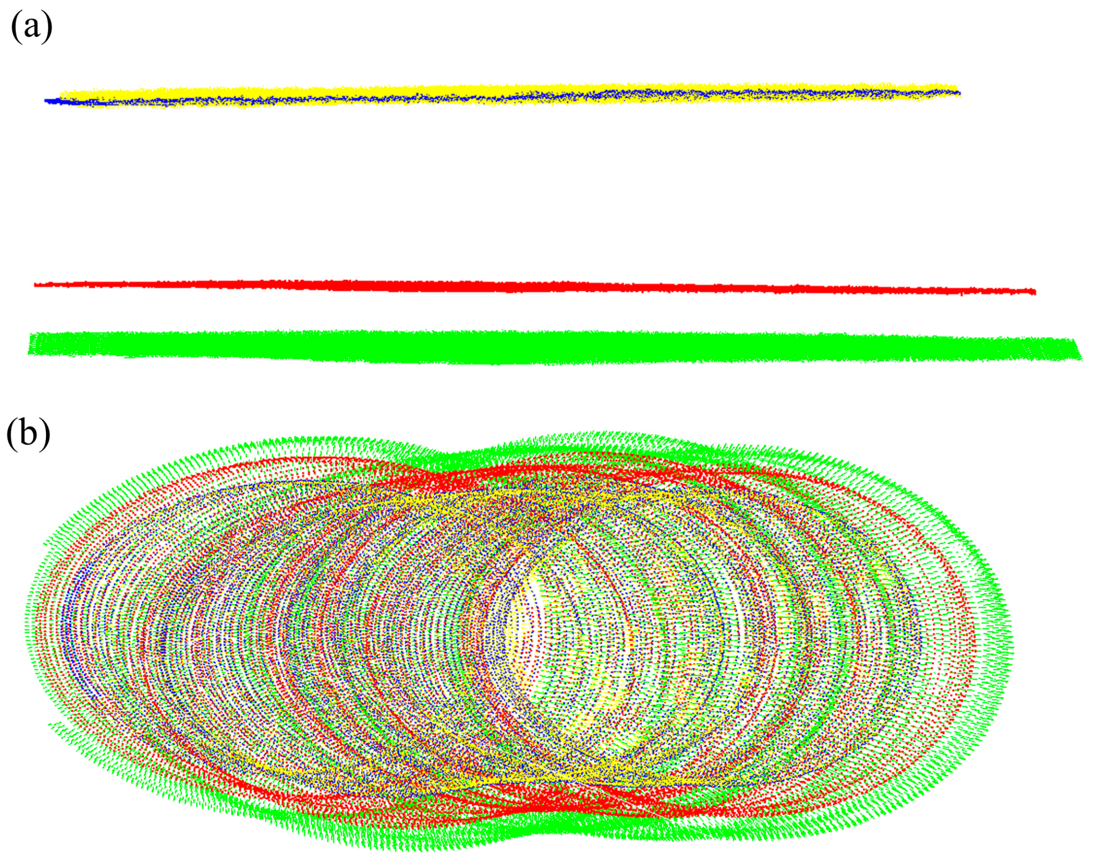
In the original waveform point cloud construction, we did not know which points were sea surface points. The point cloud solution process did not consider the seawater refraction and light propagation speed’s effect on the water. In addition, as shown in Figure 11a, the point clouds of the sea surface and seafloor after the semantic segmentation of the FWConv model were thick due to the number of points labeled with each waveform in the training sample, which was five for the sea surface and nine for the seafloor.

The waveform point clouds in the test sample were stored in an orderly text file and each waveform’s length was equal to the training set length of 300. Therefore, according to the order of the waveform point clouds stored in the file, we could know which points in each waveform were predicted by the model as the seafloor or sea surface. The points in each waveform that the model predicted as the sea surface were averaged and considered as the sea surface position, and the same operation was performed for the seafloor points. The seafloor points’ positions were then subtracted from the sea surface points’ positions and divided by 0.15 (for the distance traveled by light per unit echo moment in the air) to obtain the distances between the sea surface and seafloor moments, i.e., the slope distance information. We solved the point cloud considering the seawater refraction based on the slope distance information. The blue and red point clouds in Figure 11 are the point clouds with the seawater refraction considered, with the blue representing the sea surface point cloud and the red the seafloor point cloud. As seen in Figure 11, the seafloor point cloud without considering the seawater refraction had apparent deviations in the seawater depth and seafloor coverage; the over-thickness of the direct semantic segmentation point clouds could be solved by solving the point clouds using the slant distance.

3.5. Methods for the Evaluation

Two waveform processing methods can be compared using the FWConv method of extracting echoes. One is the ASDF method, which belongs to the same echo detection algorithm as the peak detection method for constructing samples. Compared to the peak detection method, it has a minimum distance constraint for distinguishing actual echoes from background noise, which reduces the false echo detection rate. Another method is the Richardson–Lucy deconvolution method. Wang et al. [2] showed that the Richardson–Lucy deconvolution method is efficient for handling waveforms with very shallow depths and weak bottom responses. The waveform processing results were no longer subjected to a fitting operation because the fitting did not enhance the waveform processing method’s detection capability. We tested a total of 632,807 waveforms. They were all waveforms from the portion of the strip where the Mapper4000U flew back to shore from its farthest position from the shore, overlapping with the MBES measurement area, as seen in Figure 2. All the waveforms were processed using waveform processing methods, converted to the test patterns required by FWConv, and processed using FWConv. Based on the different methods’ results, the evaluation was carried out for four aspects: (1) The sea surface points’ accuracy, which were extracted using FWConv. We carried out a plane fit to the sea surface point and used the fitted plane as a reference for the height difference between the sea surface point and the plane. (2) The extracted water depth’s correctness, including the ratio of the number of extracted water depths to the total number of waveforms, and the ratio of the number of correct extraction points to the number of extraction points. (3) The maximum water depth and point density. The maximum water depths that were extracted using the waveform processing methods were compared with the maximum water depths that were extracted using the FWConv extraction methods. The differences in the point cloud densities at different depths were also compared. (4) An accuracy analysis using MBES. The bathymetry’s accuracy was assessed by comparing the extracted bathymetric points’ elevation with the reference values. The reference value was the interpolation of MBES under the LIDAR point cloud coordinates.

4. Results

4.1. Accuracy of Sea Surface Points

The sea surface point extraction affected the refraction part of the point cloud solution, which directly influenced the seafloor points’ accuracy. We fitted the surface points to the plane and then counted the height differences from the surface points to the plane to evaluate the surface points’ accuracy. Both the waveform-processing-method- and the FWConv-extracted sea surface points were plane fitted and the height difference statistics were performed. The waveform processing method used a combination of the RLD method and peak detection, and the RLD method reduced the water body backscattering effect on the sea surface echoes. The height difference between the sea surface point and the fitted plane is defined as:

$${\delta }_s=h_s-h_p$$

(9)

where $h_s$ is the height of the fitted plane in the exact planimetric coordinates and $h_p$ is the water surface points’ height.

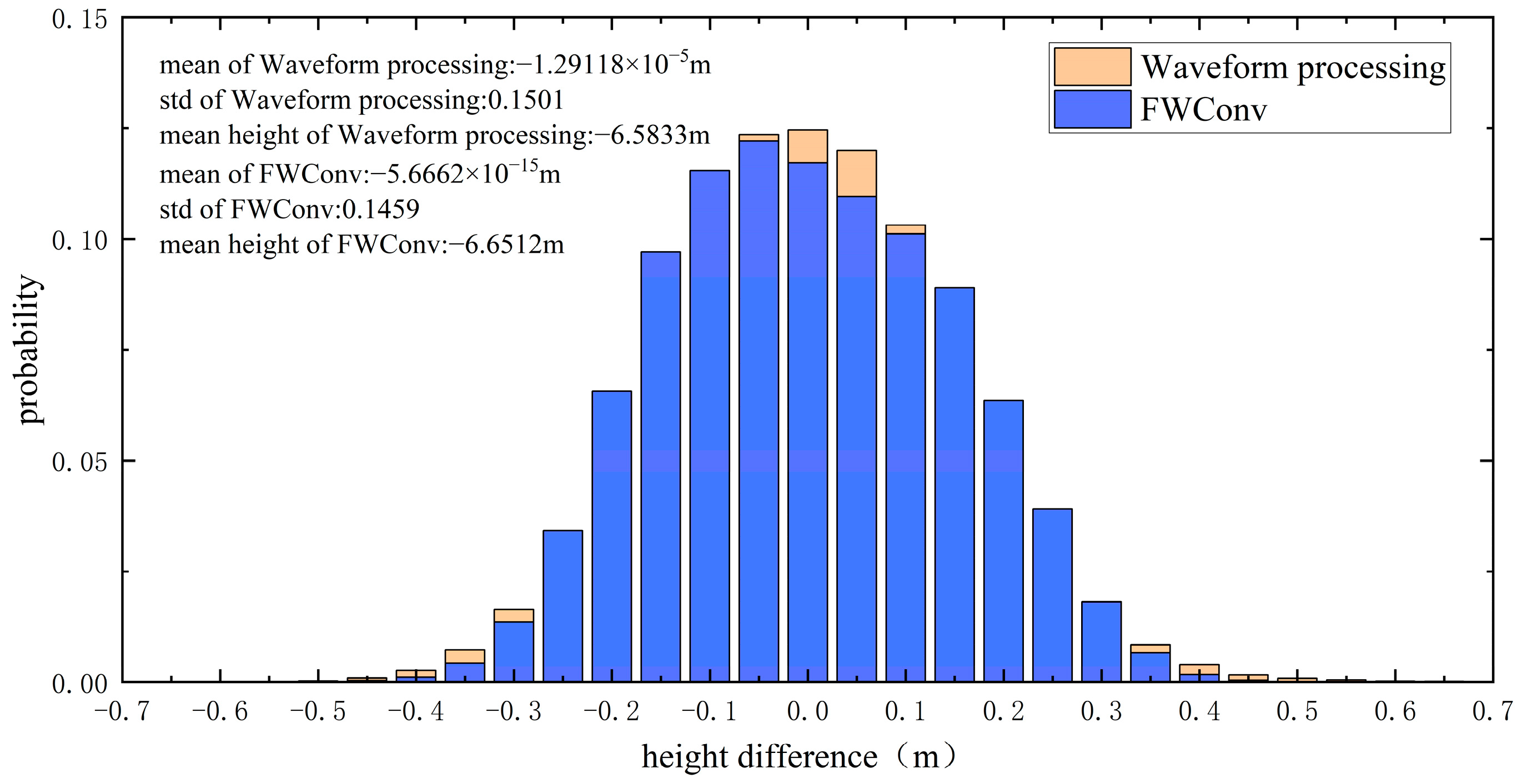
The height difference histograms of the two methods are shown in Figure 12. The height differences of both methods matched the Gaussian distribution and the standard deviation of FWConv was 0.1459, which was slightly better than that of the waveform processing, with a value of 0.1501. As seen in the mean height, the sea surface extracted using the waveform processing was 0.0679 m shallower than that extracted using FWConv, which is as it should be, because the RLD method eliminates the seawater backscattering effect to advance the sea surface peak of a waveform. In contrast, the sea surface point labeling in the FWConv training set was only constructed by the peak detection.

4.2. Detection Rate and Correctness

The waveform processing method used 3×, 5×, and 7× noise levels as the detection thresholds and considered the last echo in the waveform that satisfied the threshold condition as the seafloor echo. A waveform was considered to be detected if it outputted slope distance information after being processed using the FWConv model or the waveform processing method. The extracted slope distance information was converted into a point cloud and the points falling within 1 m of the MBES fitting plane were considered to be correctly extracted. The detection rate was defined using Equation (10) and the correctness rate was defined using Equation (11).

$$D_{\%}=N_d/N_w$$

(10)

$$C_{\%}=N_c/N_d$$

(11)

where $D_{\%}$ is the detection rate in percentage; $N_d$ is the total number of detected points; $N_w$ is the total number of waveforms; $C_{\%}$ is the correctness in percentage; and $N_c$ is the number of correct ground points.

Table 3. Detection rate and correctness.

	Ours	$7\mathit{\delta }$		$5\mathit{\delta }$		$3\mathit{\delta }$
		ASDF	RLD	ASDF	RLD	ASDF	RLD
Total number of waveforms	632,807	632,807	632,807	632,807	632,807	632,807	632,807
Detected points	537,246	624,146	626,356	631,917	628,650	632,786	628,754
Detection rate (%)	84.90	98.63	98.98	99.86	99.34	99.99	99.36
Correct points	536,296	282,231	316,193	285,113	338,334	260,999	279,166
Correctness (%)	99.82	45.22	50.48	45.12	53.82	41.25	44.40

shows the detection rate and correctness of the FWConv model and different threshold waveform processing methods. The purpose of lowering the threshold was to detect more faint echoes, but the correctness of the extracted points decreased with the threshold. ASDF achieved the highest detection rate at the $3\delta$ threshold, but also the lowest correctness. The threshold variation’s effect on the waveform processing method’s detection rate was slight, from $3\delta$ to $7\delta$, and the detection rate was maintained above 98%, while for the correctness, the threshold variation had a significant effect, from 41% to 45% for ASDF and from 44% to 53% for the RLD method. This meant that there was always a peak in the waveform that satisfied the threshold. We needed to set a higher threshold to filter the noise signal, but this would cause some of the seafloor echoes to be filtered out as well. The FWConv model predicted a detection rate of 84.90%, which was about 15% lower than that of the waveform processing method, but the extracted points’ correctness was 99.82%. The model extracted 536,296 correct points, which was 158% more than the waveform processing result. The results showed that the FWConv model could extract more seafloor points and was less susceptible to noise than the waveform processing method. The points extracted using FWConv were almost correct, which can significantly save the work of subsequent point cloud filtering.

4.3. Maximum Water Depth and Point Density

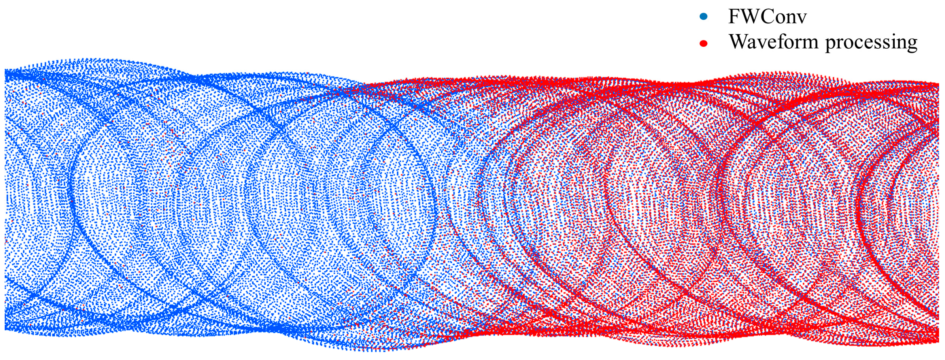
There were more points extracted using the model than the waveform processing method, including not only the points whose echo signal amplitude was above the waveform extraction threshold but were extracted incorrectly, but also the points whose echo signal was undetectable below the waveform extraction threshold. Figure 13 shows the point clouds generated using the waveform processing method and the point clouds generated using the FWConv prediction. The red point clouds were generated using the waveform processing method and the blue were generated using the FWConv model. In the right part of the figure, the waveform processing point clouds were continuously distributed in space, and there were no obvious missing point clouds on the seafloor. In the left part of the figure, due to the increase in the seawater depth and the decrease in the signal-to-noise ratio of the seafloor echo, the seafloor point clouds obtained using the waveform processing method gradually decreased, while the FWConv model could still detect at the current depth and signal-to-noise ratio.

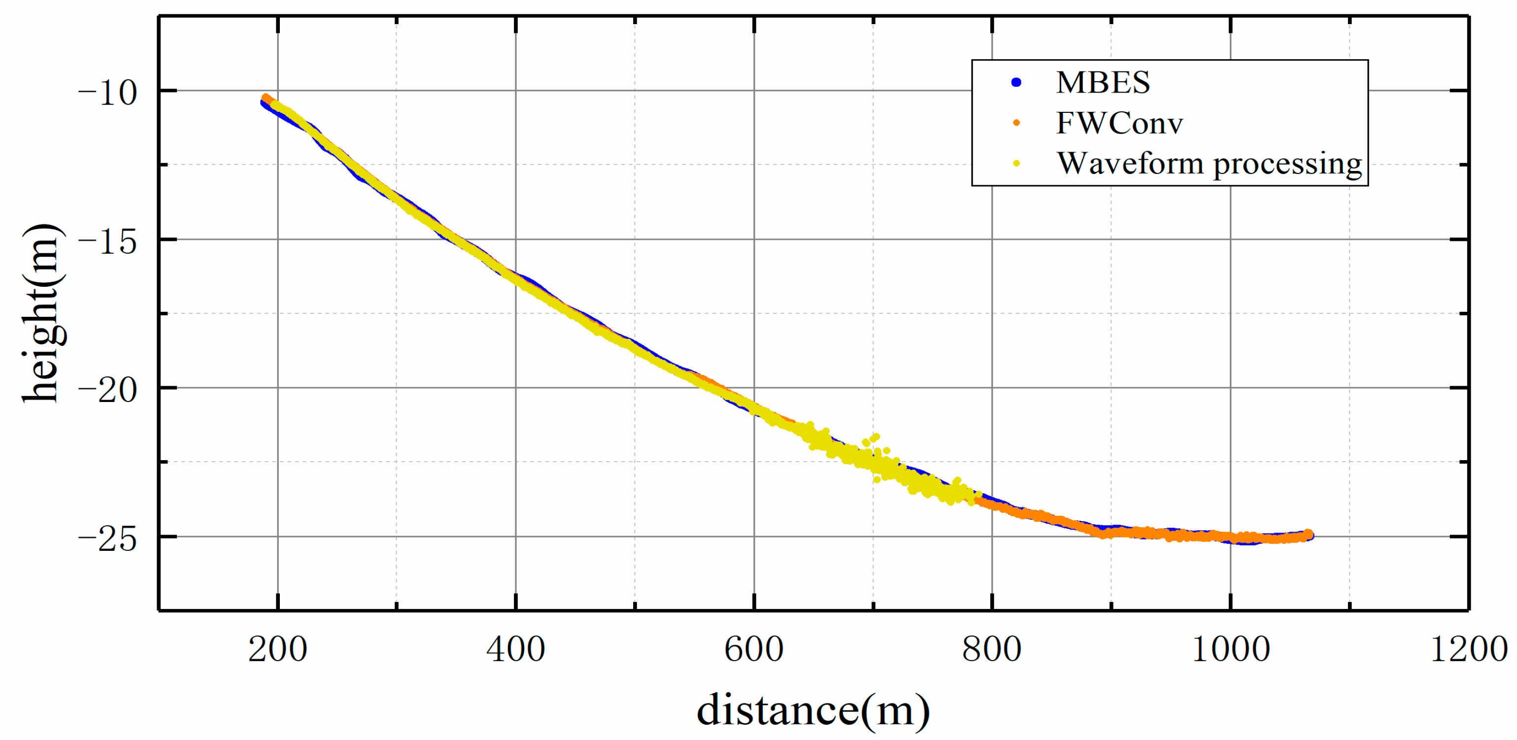
Figure 14 shows the point cloud profiles along the center of the strip obtained using the different processing methods. We averaged the sea surface heights obtained using the waveform processing and FWConv, and used this average as the reference sea surface height with a value of −6.6172 m. The point cloud generated using the waveform processing method was interrupted in the second half of the experimental strip, and the maximum measured seafloor elevation was −23.5 m, corresponding to a maximum depth of 16.88 m. The FWConv could detect the water depth in the whole experimental strip, and the predicted maximum seafloor elevation was −25.2 m, corresponding to the maximum detection depth of 18.58 m, which was 1.7 m deeper than that of the waveform processing method.

In practical application, in addition to the maximum bathymetry, there are specific requirements for the point cloud density and continuity. The maximum bathymetry is not very meaningful if only a few discrete points are at the maximum bathymetry depth. Figure 15 shows the point density distribution predicted using the waveform processing and FWConv model. Above a 13 m depth, the point cloud densities of the two methods did not significantly differ. The average point cloud density predicted using the model was 29.4 points/m², and for the waveform processing method, it was 30.1 points/m². At depths deeper than 13 m, even though the waveform processing method could extract point clouds at these depths, the mean point cloud density was small, at 2.7 points/m². The FWConv model was also affected by the reduced signal-to-noise ratio of the seafloor echo, and the point cloud density gradually decreased with the depth. However, the overall point cloud was continuously distributed and the average point cloud density reached 24.1 points/m².

4.4. Accuracy Analysis Using MBES

The points newly extracted by the model, relative to the waveform processing method, were compared to the MBES to verify the model’s prediction accuracy. The height error of the seafloor points can be expressed as:

$${\delta }_b=h_b-h_m$$

(12)

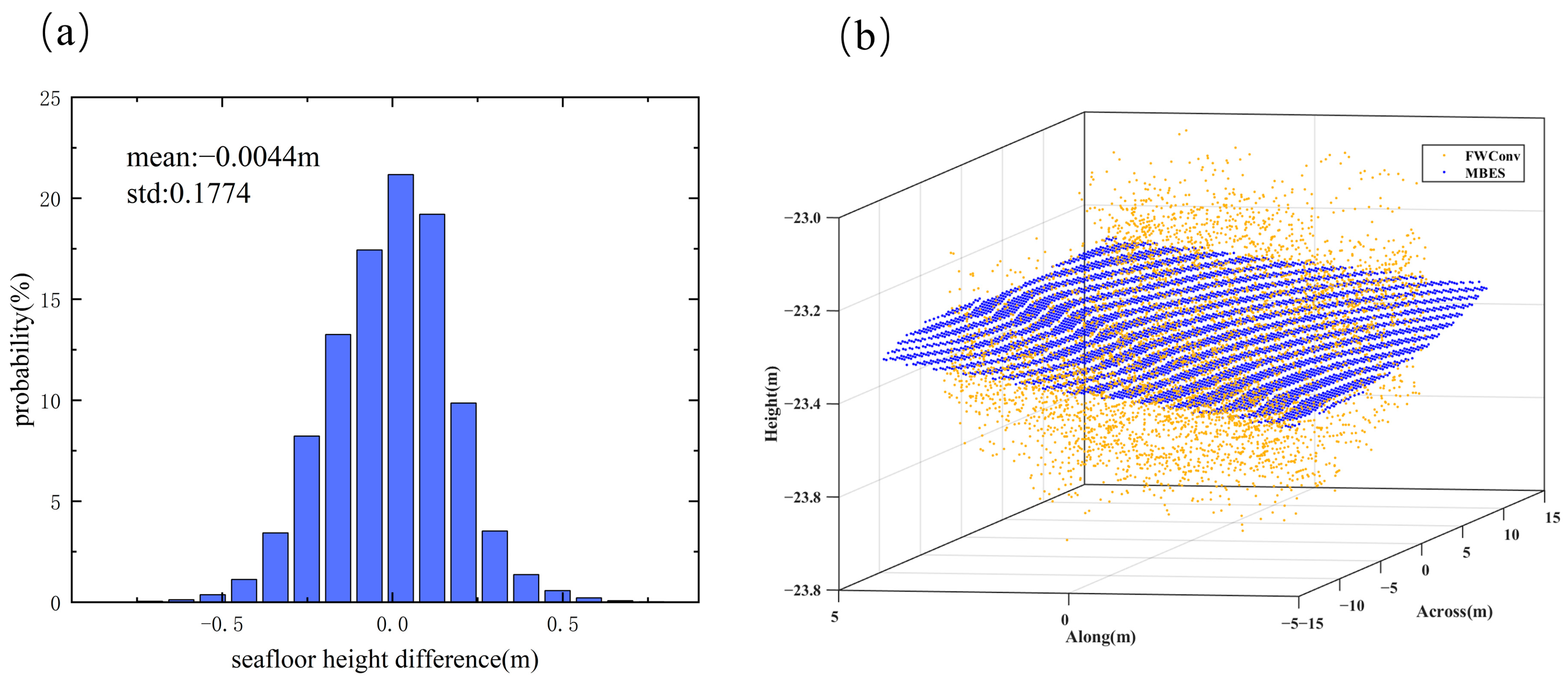
where $h_b$ is the seafloor height predicted by the model and $h_m$ is the reference height obtained using the MBES. Figure 16a expresses the histogram of the difference between the seafloor height predicted using the FWConv model and the seafloor height obtained from the MBES. The spatial distribution of a portion of the point clouds detected using the MBES and obtained using FWConv in the comparison data is shown in Figure 16b. The point cloud obtained using FWConv was distributed on both sides of the MBES and 90% of the points satisfied a ±0.3 m vertical accuracy. The mean height difference between the new measurement points and the height obtained using the MBES was −0.0044 m and the standard deviation was 0.1774.

We also compared the differences between the seafloor height points extracted using the waveform processing method (RLD) and FWConv model prediction method in the area above a 13 m water depth with those obtained using the MBES. The incorrectly extracted points from the points involved in the comparison were artificially removed. Figure 17c shows the spatial distribution of a portion of the point clouds obtained using the two methods. The point clouds obtained using both methods were distributed on both sides of the MBES, but the depth obtained using the waveform processing had a larger distribution range than that of the FWConv, as can be seen in Figure 17c. Figure 17a shows the distribution of the differences between the waveform processing methods and the MBES. The average elevation difference was −0.0742 m and the standard deviation was 0.2198 m. Figure 17b shows the distribution of the differences between the model prediction of the same point and the MBES seafloor height. The mean height difference of all the measurement points on the seafloor was 0.0623 m, with a standard deviation of 0.1345 m.

The comparison results showed that, for waveforms that could be processed using waveform processing methods (a combination of the RLD method and peak detection), the FWConv model had a higher accuracy than the waveform processing methods. Moreover, the model could extract more faint echoes, and the accuracy of these points reached less than 0.2 m.

5. Discussion

In this study, we used point cloud semantic segmentation to process LIDAR waveform data for the first time and used the FWConv model for this point cloud semantic segmentation. Assuming spatial continuity, multiple frames of the waveforms were converted into point clouds to enhance the seafloor echo information, and FWConv was used to combine the waveform intensities of adjacent frames to improve the detection capability. The abundance of the echo information in the point clouds enabled the extraction of otherwise weak signals, which is consistent with the waveform stacking results [6,7]. In essence, we utilized the waveform information from multiple frames to improve the amount of information on the seafloor. We compared the results extracted using the waveform processing method and FWConv for both the surface and bottom points. FWConv’s standard variance was smaller than that for the waveform processing, thus implying that FWConv was at least better in its precision than the compared waveform processing. When comparing the detection rate and correctness in Section 4.2, the RLD method had a better performance than ASDF, which is consistent with [2], but the correctness was lower in this paper, which could be because we only determined whether it was an echo signal using a fixed threshold, while [2] added a window size limitation. FWConv’s correctness was much higher than that of the waveform processing method, which was probably because the combination of multiple echo samples itself provided more information for the semantic segmentation of the point clouds, and because deep learning methods have a superior ability to extract point cloud features and distinguish between noises and signals.

ALB has been applied to seafloor mapping and substrate classification in shallow marine areas for effective and economical coastal protection management. However, if the airborne LIDAR bathymetry capability is insufficient, a part of the point cloud of the seafloor area will be lost, thus resulting in artifacts in the DEM of the seafloor and affecting the accuracy of the substrate classification [21,22]. Thus, the method proposed in the paper can fully utilize the waveforms to better extract weak seafloor signals, which, in turn, improves the seafloor point clouds’ completeness and reduces the artifacts generated in the seafloor’s DEM. In addition to the weak echo signal of laser echoes in the ocean, the same problem exists for the LIDAR waveform on land, where airborne LIDAR applications include archaeological research, power patrols, and topographic mapping [23,24,25]. Although the atmospheric attenuation of laser energy is much less than that of seawater, the ground echoes located under trees also suffer from weak echoes that are not easily detected due to multiple reflections of the laser from the tree canopy [26]. Therefore, the method in this paper might also be used for weak signal detection on land, but the training set needs reconstructing.

Although FWConv achieved better results than the waveform processing methods in the experimental region, some potential problems still need to be explained. FWConv’s training set in this study was composed based on the direct labeling or fitting of the waveforms obtained from the experimental region, so it can be said that FWConv only learnt the waveform features of this one water quality in the experimental region. We also trained the FWConv model without adding weak and no echo training sets. The model’s detection capability cannot detect weak echoes, which also means that the training set’s sample is quite crucial for the model’s detection capability. Therefore, if this model wants to handle the data of other water qualities, its detection ability may not reach the level of this paper. However, we believe that if we add more training samples with different water qualities and echo strengths to the training set of the model, FWConv can have a good detection capability for different water qualities. In addition, with a total of 630,000 frames tested, FWConv required about 40 min, while the waveform processing method required only two minutes. FWConv runs at 1/20th of the waveform processing’s speed, so future work will need to further streamline the FWConv model to increase its run rate.

6. Conclusions

The ocean lidar echo signal had a low signal-to-noise ratio due to the seawater’s turbidity and the seafloor substrate’s reflectivity. To extract the seafloor echoes from the faint echo data, we proposed a point cloud semantic segmentation FWConv based on the PointConv deep learning model to extract the seafloor echoes, assuming that the adjacent waveforms were geospatially correlated and had similar waveform characteristics. The major contributions of the study are: (1) a transformation of full waveforms into point clouds to combine spatially adjacent waveform features was proposed; (2) a process for extracting seafloor echoes using a point cloud semantic segmentation deep learning model was established; (3) the construction of a training set of weak seafloor echoes using waveform fitting was proposed; and (4) the comparison between waveform processing methods and the model prediction method was performed. The proposed method could extract more faint seafloor echoes and had a higher correctness than the waveform processing methods.

This study’s conclusions are: (1) the proposed method could extract the weak echo signal with a high extraction accuracy and was not easily affected by background noise; (2) the average deviation of the extracted seafloor points using the proposed method, relative to the MBES, was within 0.2 m; and (3) the proposed method could maintain a point density of 24.1 pts/m² when extracting weak seafloor signals, which was ten times higher than the waveform processing method.

In summary, the method in this paper achieved better results than the waveform processing method in the experimental area. However, there are still several aspects that need further research. The training set needs to be expanded by adding waveform samples under different water qualities to explore the model’s detection capability with regard to different water qualities. Furthermore, the study will focus on the effect of the number of waveforms contained in one sample and the number of selected neighborhood points on the model’s detection capability.

References

1. Saylam, K.; Brown, R.A.; Hupp, J.R. Assessment of depth and turbidity with airborne Lidar bathymetry and multiband satellite imagery in shallow water bodies of the Alaskan North Slope. Int. J. Appl. Earth Obs. Geoinf. 2017, 58, 191–200. [Google Scholar] [CrossRef]
2. Wang, C.S.; Li, Q.Q.; Liu, Y.X.; Wu, G.F.; Liu, P.; Ding, X.L. A comparison of waveform processing algorithms for single-wavelength LiDAR bathymetry. ISPRS J. Photogramm. Remote Sens. 2015, 101, 22–35. [Google Scholar] [CrossRef]
3. Wu, J.Y.; van Aardt, J.A.N.; Asner, G.P. A Comparison of Signal Deconvolution Algorithms Based on Small-Footprint LiDAR Waveform Simulation. IEEE Trans. Geosci. Remote Sens. 2011, 49, 2402–2414. [Google Scholar] [CrossRef]
4. Wagner, W.; Roncat, A.; Melzer, T.; Ullrich, A. Waveform analysis techniques in airborne laser scanning. In Proceedings of the ISPRS Workshop on Laser Scanning 2007 and SilviLaser 2007, Espoo, Finland, 12–14 September 2007. [Google Scholar]
5. Kogut, T.; Bakula, K. Improvement of Full Waveform Airborne Laser Bathymetry Data Processing based on Waves of Neighborhood Points. Remote Sens. 2019, 11, 1255. [Google Scholar] [CrossRef]
6. Yao, W.; Stilla, U. Mutual Enhancement of Weak Laser Pulses for Point Cloud Enrichment Based on Full-Waveform Analysis. IEEE Trans. Geosci. Remote Sens. 2010, 48, 3571–3579. [Google Scholar] [CrossRef]
7. Mader, D.; Richter, K.; Westfeld, P.; Maas, H.G. Potential of a Non-linear Full-Waveform Stacking Technique in Airborne LiDAR Bathymetry. Pfg-J. Photogramm. Remote Sens. Geoinf. Sci. 2021, 89, 139. [Google Scholar] [CrossRef]
8. Zhao, Y.Q.; Yu, X.M.; Hu, B.; Chen, R. A Multi-Source Convolutional Neural Network for Lidar Bathymetry Data Classification. Mar. Geod. 2022, 45, 232–250. [Google Scholar] [CrossRef]
9. Kogut, T.; Slowik, A. Classification of Airborne Laser Bathymetry Data Using Artificial Neural Networks. IEEE J. Sel. Top. Appl. Earth Obs. Remote Sens. 2021, 14, 1959–1966. [Google Scholar] [CrossRef]
10. Roshandel, S.; Liu, W.Q.; Wang, C.; Li, J. Semantic Segmentation of Coastal Zone on Airborne Lidar Bathymetry Point Clouds. IEEE Geosci. Remote Sens. Lett. 2022, 19, 1–5. [Google Scholar] [CrossRef]
11. Wang, D.D.; Xing, S.; He, Y.; Yu, J.Y.; Xu, Q.; Li, P.C. Evaluation of a New Lightweight UAV-Borne Topo-Bathymetric LiDAR for Shallow Water Bathymetry and Object Detection. Sensors 2022, 22, 1379. [Google Scholar] [CrossRef]
12. Allouis, T.; Bailly, J.S.; Pastol, Y.; Le Roux, C. Comparison of LiDAR waveform processing methods for very shallow water bathymetry using Raman, near-infrared and green signals. Earth Surf. Process. Landf. 2010, 35, 640–650. [Google Scholar] [CrossRef]
13. Abdallah, H.; Bailly, J.S.; Baghdadi, N.N.; Saint-Geours, N.; Fabre, F. Potential of Space-Borne LiDAR Sensors for Global Bathymetry in Coastal and Inland Waters. IEEE J. Sel. Top. Appl. Earth Obs. Remote Sens. 2013, 6, 202–216. [Google Scholar] [CrossRef]
14. Xing, S.; Wang, D.D.; Xu, Q.; Lin, Y.Z.; Li, P.C.; Jiao, L.; Zhang, X.L.; Liu, C.B. A Depth-Adaptive Waveform Decomposition Method for Airborne LiDAR Bathymetry. Sensors 2019, 19, 5065. [Google Scholar] [CrossRef] [PubMed]
15. Zhao, X.L.; Liang, G.; Liang, Y.; Zhao, J.H.; Zhou, F.N. Background noise reduction for airborne bathymetric full waveforms by creating trend models using Optech CZMIL in the Yellow Sea of China. Appl. Opt. 2020, 59, 11019–11026. [Google Scholar] [CrossRef] [PubMed]
16. Nie, S.; Wang, C.; Li, G.C.; Pan, F.F.; Xi, X.H.; Luo, S.Z. Signal-to-noise ratio-based quality assessment method for ICESat/GLAS waveform data. Opt. Eng. 2014, 53, 103104. [Google Scholar] [CrossRef]
17. Guo, Y.L.; Wang, H.Y.; Hu, Q.Y.; Liu, H.; Liu, L.; Bennamoun, M. Deep Learning for 3D Point Clouds: A Survey. IEEE Trans. Pattern Anal. Mach. Intell. 2021, 43, 4338–4364. [Google Scholar] [CrossRef]
18. Qi, C.R.; Yi, L.; Su, H.; Guibas, L.J. PointNet plus plus: Deep Hierarchical Feature Learning on Point Sets in a Metric Space. In Proceedings of the 31st Annual Conference on Neural Information Processing Systems (NIPS), Long Beach, CA, USA, 4–9 December 2017. [Google Scholar]
19. Wu, W.X.; Qi, O.G.; Li, F.X.; Soc, I.C. PointConv: Deep Convolutional Networks on 3D Point Clouds. In Proceedings of the 32nd IEEE/CVF Conference on Computer Vision and Pattern Recognition (CVPR), Long Beach, CA, USA, 16–20 June 2019; pp. 9613–9622. [Google Scholar]
20. Lin, T.Y.; Goyal, P.; Girshick, R.; He, K.M.; Dollar, P. Focal Loss for Dense Object Detection. IEEE Trans. Pattern Anal. Mach. Intell. 2020, 42, 318–327. [Google Scholar] [CrossRef]
21. Do, J.D.; Jint, J.Y.; Kim, C.H.; Kim, W.H.; Lee, B.G.; Wie, G.J.; Chang, Y.S. Measurement of Nearshore Seabed Bathymetry using Airborne/Mobile LiDAR and Multibeam Sonar at Hujeong Beach, Korea. J. Coast. Res. 2020, 95, 1067–1071. [Google Scholar] [CrossRef]
22. Janowski, L.; Wroblewski, R.; Rucinska, M.; Kubowicz-Grajewska, A.; Tysiac, P. Automatic classification and mapping of the seabed using airborne LiDAR bathymetry. Eng. Geol. 2022, 301, 106615. [Google Scholar] [CrossRef]
23. Liu, F.H.; He, Y.; Chen, W.B.; Luo, Y.; Yu, J.Y.; Chen, Y.Q.; Jiao, C.M.; Liu, M.Z. Simulation and Design of Circular Scanning Airborne Geiger Mode Lidar for High-Resolution Topographic Mapping. Sensors 2022, 22, 3656. [Google Scholar] [CrossRef]
24. Štular, B.; Lozić, E. Airborne LiDAR data in landscape archaeology. Introd. Non-Archaeol. 2022, 64, 247–260. [Google Scholar]
25. Van Den Eeckhaut, M.; Poesen, J.; Verstraeten, G.; Vanacker, V.; Nyssen, J.; Moeyersons, J.; van Beek, L.P.H.; Vandekerckhove, L. Use of LIDAR-derived images for mapping old landslides under forest. Earth Surf. Process. Landf. 2007, 32, 754–769. [Google Scholar] [CrossRef]
26. Magruder, L.A.; Neuenschwander, A.L.; Marmillion, S.P. Lidar waveform stacking techniques for faint ground return extraction. J. Appl. Remote Sens. 2010, 4, 043501. [Google Scholar] [CrossRef]
Figure 1. The appearance of Mapper4000U.
Remotesensing 15 02326 g001
Figure 2. Study area. The red line represents the aircraft trajectory of the Mapper4000U, and the range contained by the blue dashed line is the working area of the ship measurement multibeam echo sounder. The colors correspond to the elevation of the seafloor in the experimental area.
Remotesensing 15 02326 g002
Figure 3. Workflow of point cloud generation using FWConv.
Remotesensing 15 02326 g003
Figure 4. Typical waveform bin labeling results. The blue dots are bin values labeled as background. The red dots are bin values labeled as seafloor, and the pink dots are bin values labeled as surface.
Remotesensing 15 02326 g004
Figure 5. The final constructed faint echo waveform. The yellow line represents the waveform fitted to the measured data. The blue line is the noise and Gaussian function added to the fit. The red dots are the seafloor points labeled according to the Gaussian function positions.
Remotesensing 15 02326 g005
Figure 6. (a) Scanning module of Mapper4000U. (b) Mechanism of point cloud generation for Mapper 4000U. The path of the laser ray is the blue line.
Remotesensing 15 02326 g006
Figure 7. (a) Scan trajectory of Mapper4000U. (b) Waveform point cloud for the flight trajectory conversion of (a). (c) Training sample for a certain angle in the scan trajectory. (d) The labeled results corresponding to the training samples in (c).
Remotesensing 15 02326 g007
Figure 8. The process of conducting PointConv on one local region centered around one point p 0 , f 0 .
Remotesensing 15 02326 g008
Figure 9. Problem statement to be solved using FWConv. Our model predicts the probability of each class for each input consisting of coordinates and amplitude.
Remotesensing 15 02326 g009
Figure 10. FWConv architecture.
Remotesensing 15 02326 g010
Figure 11. (a) Front view of the point cloud. (b) Top view of the point cloud (yellow points are the surface points of the model semantic segmentation and green points are the bottom points of the model semantic segmentation. Blue points are surface points with seawater refraction considered; red points are seafloor points with seawater refraction considered).
Remotesensing 15 02326 g011
Figure 12. Probability distribution of the difference in the sea surface height for the two methods.
Remotesensing 15 02326 g012
Figure 13. Point clouds of the seafloor generated using different methods.
Remotesensing 15 02326 g013
Figure 14. The point cloud profiles along the center of the strip. The X-axis is the distance from the shore.
Remotesensing 15 02326 g014
Figure 15. Point density at different water depths.
Remotesensing 15 02326 g015
Figure 16. (a) Distribution of the difference between the seafloor height predicted using the model and the seafloor height obtained from using MBES; and (b) the spatial distribution of the point clouds detected using MBES and those obtained using FWConv.
Remotesensing 15 02326 g016
Figure 17. (a) Difference distribution of waveform processing method and MBES; (b) difference distribution of model prediction and MBES; and (c) spatial distribution of point clouds from different methods.
Remotesensing 15 02326 g017