Article

Explainable Artificial Intelligence (XAI) Model for Earthquake Spatial Probability Assessment in Arabian Peninsula

by
Ratiranjan Jena
1,*,
Abdallah Shanableh
1,2,
Rami Al-Ruzouq
1,2,
Biswajeet Pradhan
3,
Mohamed Barakat A. Gibril
1,2,
Mohamad Ali Khalil
1,
Omid Ghorbanzadeh
4,
Ganapathy Pattukandan Ganapathy
5 and
Pedram Ghamisi
6
1
GIS & Remote Sensing Center, Research Institute of Sciences and Engineering, University of Sharjah, Sharjah 27272, United Arab Emirates
2
Civil and Environmental Engineering Department, University of Sharjah, Sharjah 27272, United Arab Emirates
3
Centre for Advanced Modelling and Geospatial Information Systems (CAMGIS), School of Civil and Environmental Engineering, Faculty of Engineering and Information Technology, University of Technology Sydney, Sydney, NSW 2007, Australia
4
Institute of Advanced Research in Artificial Intelligence (IARAI), Landstraßer Hauptstraße 5, 1030 Vienna, Austria
5
Centre for Disaster Mitigation and Management, Vellore Institute of Technology, Vellore 632 014, Tamil Nadu, India
6
MachineLearning Group, Helmholtz Institute Freiberg for Resource Technology, Helmholtz-Zentrum Dresden-Rossendorf, Chemnitzer Str. 40, 09599 Freiberg, Germany
*
Author to whom correspondence should be addressed.
Remote Sens. 2023, 15(9), 2248; https://doi.org/10.3390/rs15092248
Submission received: 14 February 2023 / Revised: 6 April 2023 / Accepted: 21 April 2023 / Published: 24 April 2023

Abstract

:
Among all the natural hazards, earthquake prediction is an arduous task. Although many studies have been published on earthquake hazard assessment (EHA), very few have been published on the use of artificial intelligence (AI) in spatial probability assessment (SPA). There is a great deal of complexity observed in the SPA modeling process due to the involvement of seismological to geophysical factors. Recent studies have shown that the insertion of certain integrated factors such as ground shaking, seismic gap, and tectonic contacts in the AI model improves accuracy to a great extent. Because of the black-box nature of AI models, this paper explores the use of an explainable artificial intelligence (XAI) model in SPA. This study aims to develop a hybrid Inception v3-ensemble extreme gradient boosting (XGBoost) model and shapely additive explanations (SHAP). The model would efficiently interpret and recognize factors’ behavior and their weighted contribution. The work explains the specific factors responsible for and their importance in SPA. The earthquake inventory data were collected from the US Geological Survey (USGS) for the past 22 years ranging the magnitudes from 5 Mw and above. Landsat-8 satellite imagery and digital elevation model (DEM) data were also incorporated in the analysis. Results revealed that the SHAP outputs align with the hybrid Inception v3-XGBoost model (87.9% accuracy) explanations, thus indicating the necessity to add new factors such as seismic gaps and tectonic contacts, where the absence of these factors makes the prediction model performs poorly. According to SHAP interpretations, peak ground accelerations (PGA), magnitude variation, seismic gap, and epicenter density are the most critical factors for SPA. The recent Turkey earthquakes (Mw 7.8, 7.5, and 6.7) due to the active east Anatolian fault validate the obtained AI-based earthquake SPA results. The conclusions drawn from the explainable algorithm depicted the importance of relevant, irrelevant, and new futuristic factors in AI-based SPA modeling.

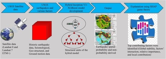
Graphical Abstract

1. Introduction

Earthquakes are one of the most critical, and destructive natural hazards that can last for a few seconds, but the impact stays for years or even decades. According to the National Earthquake Information Center (NEIC), around 20,000 earthquakes are occurring each year worldwide [1]. Since the 1900s, geologists and seismologists expect about 16 major earthquakes that could affect over a billion people [2]. The Arabian Peninsula is one of the driest inhabited continents, which has experienced several earthquakes due to the Zagros–Bitlis fold and fault belt, Red Sea, Gulf of Aden, and Arabian/Persian Gulf [3]. There is a possibility that future events of high magnitude will occur in this region.
The basic definition of earthquake spatial probability is a potential location for a particular magnitude event to occur within a specific period. Seismic hazard is the probability of ground shaking due to earthquakes [4]. However, the definition is quite complicated as it changes with time and space [5]. Two major types of hazard assessment techniques are often used globally such as probabilistic (PSHA) and deterministic seismic hazard assessment (DSHA) [6,7]. Particularly, the statistical models are commonly used in PSHA to estimate the probability, whereas DSHA accentuates the ground shaking, based on physical models.
Globally, some works demonstrated that in a quantitative earthquake probability study, the incorporation of fault interaction and stress triggering is necessary. These studies implemented novel techniques to derive earthquake probability using the stress changes which is used with fault models [8,9]. Shcherbakov et al. [10] conducted a study to compute extreme earthquake probabilities above a certain magnitude. The study shows that the occurrence of unexpected earthquakes could trigger powerful subsequent earthquakes. The results of their study could be useful in estimating earthquake probabilities in several stages of a sequence of events. Schäfer and Wenzel [11] conducted a global earthquake temporal probability assessment using multi-variate ML. Their results showed the potential of megathrust events in Manus Adriatic Thrust, and Mussau Trenches, where no historical earthquakes have been recorded. Gitis and Derendyaev [12] implemented an ML method of the minimum area of alarm and a method of approximation of interval expert for probability estimation. They successfully forecasted the target magnitudes based on an automatic web-based platform. Jena et al. [13] implemented a deep learning technique to estimate earthquake probability and achieved 89.47% accuracy in Palu, Indonesia. In another work, Jena et al. [14] applied a deep learning-based spatial probability assessment (SPA) in NE India and obtained 94% accuracy. Jena et al. [15] proposed an integrated model of artificial neural network analytical hierarchy process (ANN-AHP) for earthquake probability and risk assessment in Aceh province, Indonesia. The study observed that a high probability can be found in the southwest portion of the city using the ANN technique having an overall accuracy of 84%. In more recent work, Pourghasemi et al. [16] conducted a study on multi-hazard probability assessment in Iran using ensemble ML techniques. They achieved an overall accuracy of more than 80% for earthquake probability estimation. This implies that the use of ML techniques is becoming increasingly popular among geoscientists and hazard modelers due to its incremental learning process and high level of accuracy.
In the Arabian Peninsula, to the extent of our knowledge, no earthquake SPA analyses for magnitudes above 5 Mw have been conducted. For instance, the two major studies were executed by Al-Haddad et al. [17,18] to generate seismic design standards for Saudi Arabia based on a probabilistic approach for PGA estimation. Later, they enlarged the PGA values for the whole Arabian Peninsula. Without considering the tectonic nature, a single ground-motion prediction equation (GMPE) was implemented. According to their results, the southernmost and western parts of the Zagros Belt and Makran Subduction Zone (MSZ) fall under the high-hazard zone, respectively. The Zagros–Bitlis Belt in the southeast and northwest has encountered a geodetical shortening of about 10 mm/year and 5 mm/year, respectively [19,20]. Further, they estimated the PGA values for 475 and 2475 years of the return period. However, the observed PGA was not well correlated with the damage potential of ground shaking. The third study was performed by Pascucci et al. (2008) on hazard estimation without considering the active fault map of Iran [21] in the seismic source model. This work did not produce the iso-acceleration maps for the entire Arabian Peninsula. Their study estimated hazard values for some cities in UAE, Saudi Arabia, Qatar, and Bahrain. In another work, Al-Shijbi et al. [22] performed a PSHA for the Arabian Peninsula. Their study observed the highest ground acceleration values along the Zagros, the East Anatolian Fault, and the Gulf of Aqaba–Dead Sea Fault. The East Anatolian Fault separates the Arabian Plate from the Anatolian Plate resulting in high-magnitude events [23]. The Red Sea shows evidence of continental rifting and falls under a high-hazard zone. Numerous other seismic hazard assessments have been conducted in the Arab Peninsula [24,25,26,27]. Generally, most parts of the Arabian Peninsula are covered by low-to-moderate hazard zone as reported in the aforementioned studies. A smaller region falls under high hazard levels because of poor building quality. Geophysical studies conducted in the Gulf of Aden are characterized by an oceanic crust, indicating a high-hazard zone [28].
The hindrance to applying ML models in earthquake probability management studies is to achieve high prediction accuracy [29,30]. Moreover, the investigations face challenges such as a lack of transparency and explainability of the results, due to the black-box nature of the applied ML models [31]. The SHAP explainability approach describes the internal function of the Inception v3-XGBoost model to estimate the factors’ interaction, relative importance, stable factors, local contribution, the distance among explanations, and predict the individual factors information on a single prediction, respectively. The physical models are widely used in the literature for seismological studies; however, several studies have found that AI-based models outperform them [13,14]. Moreover, the traditional probabilistic models assume an attenuation relation for all the events and locations with an unrealistic hypothesis for PGA estimation having uncertainties [32]. In the literature, we did not come across any work on the application of AI techniques in SPA in the Arabian Peninsula. The emergence of new explainable algorithms, such as SHAP, is useful to understand model and factors interaction that changed the perception of using AI-based models [33]. Because SHAP works more robustly for all ML models than other XAI models such as Local Interpretable Model-Agnostic Explanations (LIME) and generalized additive model (GAM) [34].
The aim and novelty of the work lie in the application of an XAI framework to estimate earthquake spatial probability and identify the contributing factors, hidden interaction, and their relative importance. The current study attempted to leverage the use of the XAI technique to explain the black-box nature of the ML models. Hence, the present study focuses on estimating and understanding the SPA outputs using SHAP plots. No updated probability maps in the Gulf of Aqaba–Dead Sea Fault can be seen after Al-Haddad et al. [20] published a temporal probability map. However, no study has been conducted for a comprehensive SPA in the Gulf of Aden, Red Sea, which makes this study different from others. In summary, the objectives of the work are to: (i) use a hybrid Inception v3-ensemble XGBoost model to estimate earthquake spatial probability index; (ii) analyze the lone predictions using SHAP outputs to understand the predictors’ interaction for earthquake SPA; and (iii) examine the spatial variation of outputs on change in factors and geographic conditions. This study addresses the following research questions: (1) how XAI works to apprehend and comprehend the model decisions, and complex intrinsic non-linear relations, respectively; and (2) ascertain the models’ suitability for earthquake probability mapping.

2. Study Area

The Arabian Peninsula is bordered by active tectonic margins [35]. The selected buffer area (2000 km radius) is centroid by Saudi Arabia and unexplored/partially explored that considers the major thrust faults and tectonic contacts. Divergent boundaries can be found along the Red Sea and the Gulf of Aden. Major transform plate boundaries are situated along the East Anatolian Fault, Owen Fracture Zone, and the Gulf of Aqaba–Dead Sea Fault Zone [24]. The active convergent plate boundaries are located in the Makran Subduction Zone (MSZ), where the Arabian Plate subducts beneath the Eurasian plate producing a collision zone of the Zagros–Bitlis Fold Thrust Belt [36,37].
Seismic activity is mostly confined to plate boundaries in the Arabian Peninsula. Some studies mentioned that the Arabian Plate is a stable craton [26,38], however small magnitude events were observed from Palmyra, Sinjar area, and Oman mountains. Additionally, small-to-moderate earthquakes are observed within the Peninsula [35]. The MSZ is dominated by shallow-depth earthquakes (30 km). The northward MSZ develops broad north dipping thrust faults and deformation zone. Hessami et al. [23] revealed that the MSZ dips at an angle of 6° northwards, where the deeper dip angle was observed at 19°. An ongoing drift makes the Arabian Peninsula spread at a rate of approximately 16 mm/year [39]. The Gulf of Aden is a seafloor spreading environment, where the Arabian Plate is moving away from the African Plate. Therefore, all the tectonic movements are responsible for many earthquakes along the active plate boundaries around the Arabian Peninsula (Figure 1a,b).

3. Materials and Methods

3.1. Data

In this study, the major inputs were derived from reliable seismological, geological, geostructural, and ground motion data. This study implemented a procedure originally developed by Wason et al. [40] to convert all forms of magnitudes into moment magnitudes (Mw). First, earthquake catalogs were collected from several databases, including the National Earthquake Information Center (NEIC), the National Centre for Seismology (NCS), and the United States Geological Survey (USGS). The data collection period was from 2000 until 2022 with a filtered threshold of magnitude 5 Mw and above to avoid incompleteness. The inventory data were applied for training and validation purposes in the Inception v3-extreme gradient boosting (Inception v3-XGBoost) model. Second, several factors were generated in the GIS environment. Third, administrative boundary, digital elevation model (DEM), thrust faults, tectonic contacts, and geology data were acquired by using remote sensing images and shape files. Fault information was derived using Landsat ETM+ and geology was derived using Landsat data. The earthquake SPA map for the Arabian Peninsula was generated using ArcGIS 10.8 and Python 3.9. To generate the thematic layers and training purposes, different algorithms, such as inverse distance weighting (IDW), spline, Euclidian distance, Kernel density, and buffer were used.
Developed thematic layers based on the natural breaks classification technique can be explained through objective themes, concepts of conditioning factors, prominent patterns, and insight prediction logic. Data pre-processing was conducted to remove some negative and illogical values. Subsequently, all the thematic maps were extracted into multiple values using ArcGIS tools. Each pixel value was produced in association with the target values to process. Next, post-processing was conducted after the prediction task using a point-to-raster conversion tool in ArcGIS software to generate a raster map. The major earthquakes in the Arabian Shield (Mw 6.5), Dead Sea (Mw 7.8), Red Sea (Mw 7.9), Gulf of Aden (Mw 6.7), Makran subduction zone (Mw 8.4) are recorded and the detail earthquake information in the Arabian shield is presented in Table 1. The details about data sources, input factors, methods, and importance are presented in Table 2.

3.2. Methodology

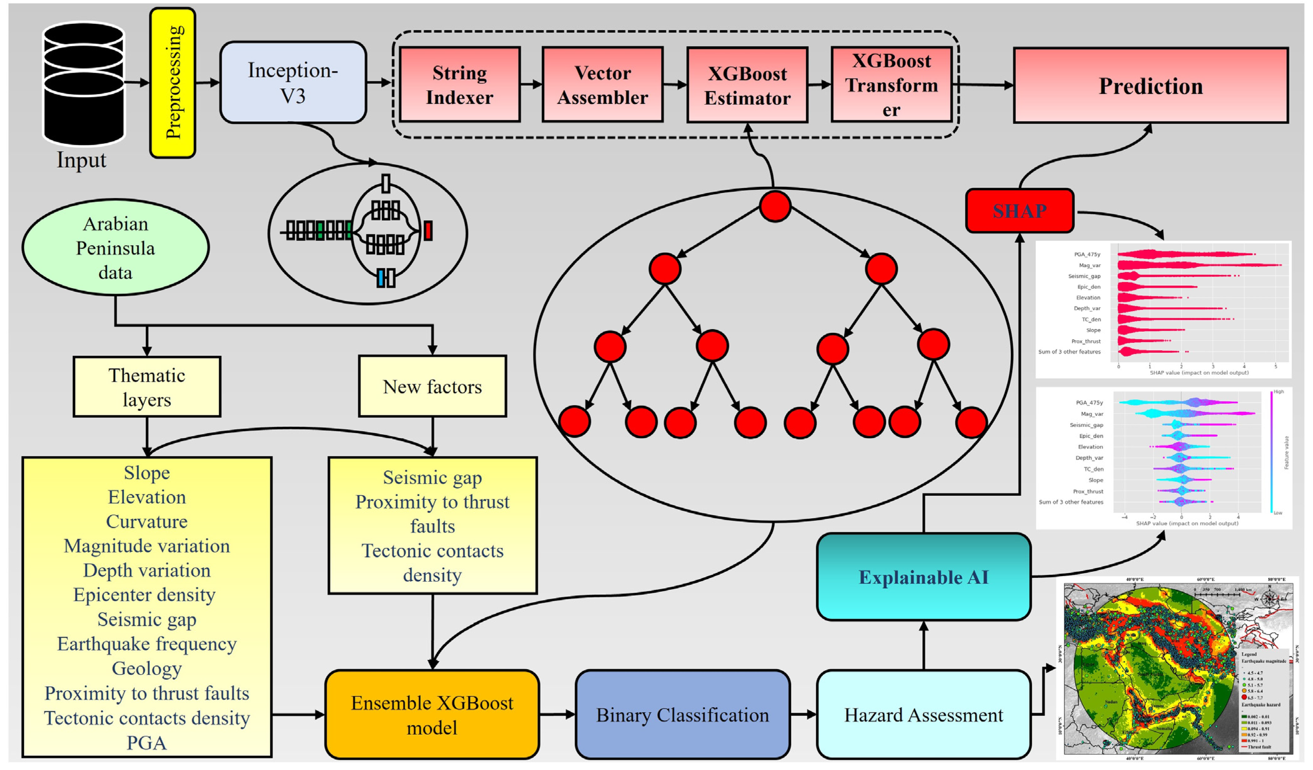
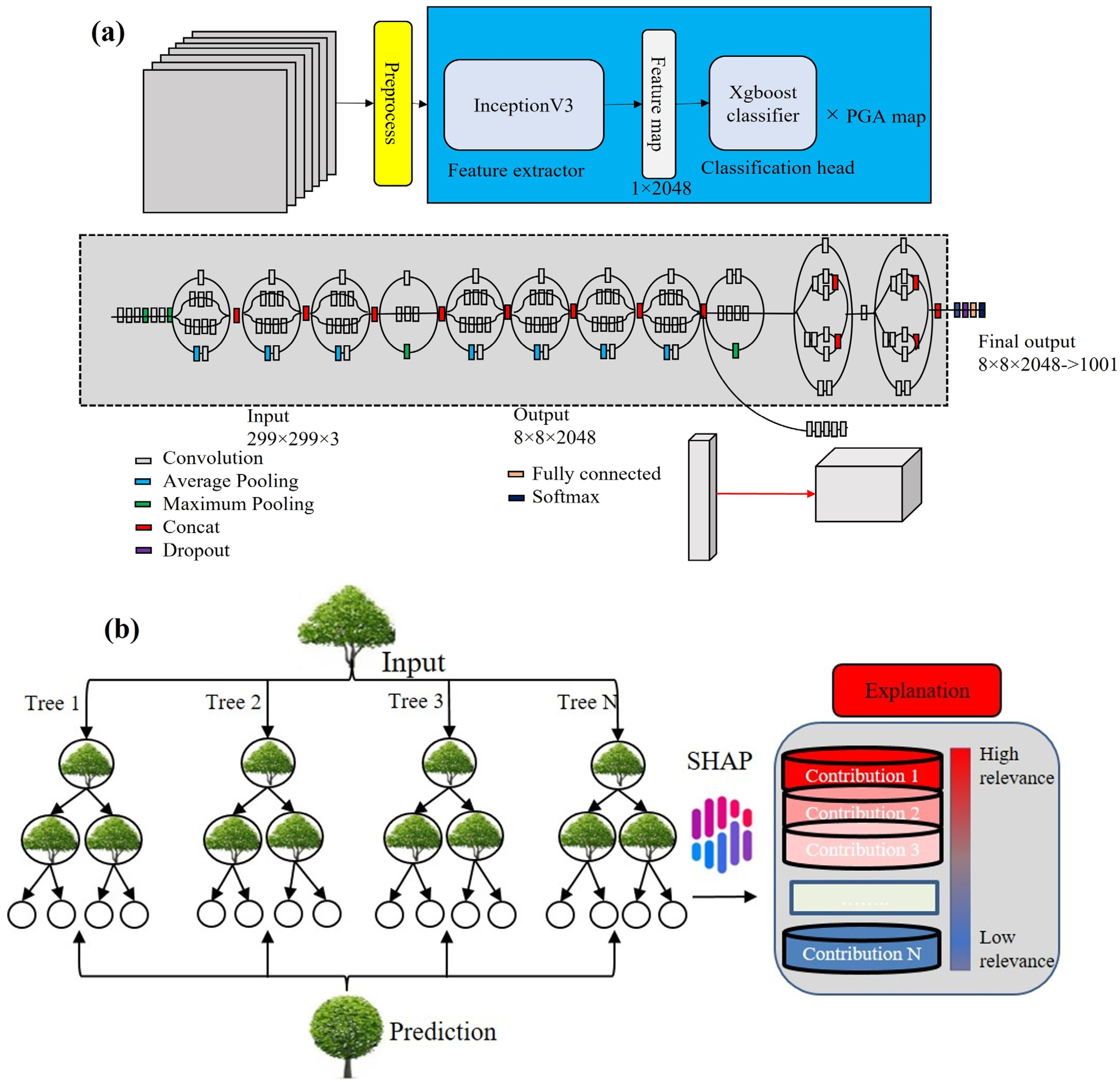
This study proposed a hybrid Inception V3-XGBoost model (Figure 2). The architecture of the Inception v3-XGBoost model is shown in Figure 3a. The designed model is characterized by a feature extractor and a classification head [50]. This model replaced the classification head in the inception V3 model with the XGBoost classifier (Figure 3b). The input features provided by the Inception V3 model were used for the XGBoost classifier. This setup of hybrid combination works for other pre-trained CNNs and RNN models too. In the first stage, the Inception v3 model was fine-tuned for the training dataset. This study observed that the information originating from Inception v3 leads to a better result by the XGBoost classifier.
This implemented Inception v3-XGBoost model is used to predict the targets, such as earthquake points and non-earthquakes, through Inception v3 and string indexer, vector assembler, XGBoost estimator, XGBoost transformer [51]. To make a close of the predicted value with the real value in each round, trees are constructed based on the output of the previous tree, to enhance the model’s prediction performance. Then, pre-processing of the data set is necessary to avoid interference with classification results because of null values, unbalanced data, different data structures, etc. Hereafter, feature selection can be applied to the data. Training, testing, and evaluation can be performed.
Then, the SHAP library was implemented using JavaScript functions to estimate the contribution of factors towards hazard assessment and factors interaction. Therefore, we explored how variables affect the model output by using individual and collective summary plots. Thereafter, a comparative study was conducted among the SHAP findings with or without important factors, and the influence of the factor “seismic gap” on earthquake hazard was estimated. This research has been conducted by using a combined approach of an ensemble boosting algorithm (XGBoost) and an explainable AI named SHAP. The steps are mentioned in detail in Figure 2.

3.2.1. Inception V3 Model Architecture

The network of Inception-v3 is a deep learning model [50]. The difficulty occurs in training the model directly using a low-configured computer if there is no access to a supercomputer. Therefore, Inception-v3 works well through transfer learning, and the main graph of the Inception-v3 model can be presented in Figure 3. The TensorFlow library was used to retrain Inception’s final layer for new categories. The transfer learning approach is a knowledge gaining method that uses the previous layer’s parameters and removes the end layer, then retrains the last layer. The last layer output nodes are equal to the number of dataset categories. If the dataset has 1000 classes, 1000 output nodes can be observed in the last layer in the original model. Therefore, for the final classification purposes (0,1), this study applied the XGBoost classifier. The details of the XGBoost classifier were explained using the mathematical expression as shown in Section 4.2.
Here, the model loss can be presented as follows:
L o s s = i N l o s s ( i , c l a s s i ) i N w e i g h t ( c l a s s i )
Training CNNs often generates results in overfitting. Therefore, this study implemented pre-trained CNNs to avoid this problem. The most popular CNN architectures are being used as ResNet and DenseNet. However, the best CNNs model that this study employed is the Inception-v3 model which is initialized by random weights and fine-tuned on the dataset to extract features. The Inception v3 is a pre-trained CNN model that provided the best F1 score. This model is the 3rd version of the inception family CNN models characterized by several improvements. This model provides an improved factorized convulsion which reduces the number of parameters and maintains network efficiency. This model uses a regularizer for label smoothing. Additionally, an auxiliary classifier was also employed to help propagate label information and regularization.

3.2.2. XGBoost Model Architecture

XGBoost is an ensemble machine learning model, a gradient boost algorithm, used to improve the performance of model prediction that combines a sequence of weak models into a strong learning model [52]. The ensemble models provide better results compared to a single model (Figure 3).
In this section, the steps of XGB algorithm implementation were described [53].
Step 1: Initialization
For solving a binary classification problem, where y i is the actual label can be represented as 1 or 0. Therefore, the most used log loss function can be considered in this case, can be presented as:
l y i , y ^ i t = y i log P i + 1 y i log 1 P i .
where
p i = 1 1 + e y ^ i ( t ) .
According to P i , y i and p values, g i and h i values can be estimated. where
g i = P i y i , h i = p 1 p i .
from the ( t 1 ) th tree of sample x i , the estimated predicted value can be presented as y ^ i ( t 1 ) , where the actual value of x i is y i . However, the prediction value will be 0 for the 0th tree which means y ^ i ( 0 ) = 0 .
Step 2: The Gain value of features needs to traverse through and be calculated to determine the splitting mode for the current root node. The Gain value will help to estimate the feature node with the maximum Gain score.
Step 3: In this step, the establishment of the Current Binary Leaf Node setup can be conducted. According to the feature with maximum Gain, the sample set is classified into two parts to obtain two leaf nodes. In addition, the second step should be repeated for two leaf nodes by considering the negative gain score and stopping conditions, respectively. This step led to establishing the whole tree [53].
Step 4: Whole Leaf Node prediction values can be calculated in this step. Leaf node ω j prediction values can be calculated as:
ω j = G j H j + λ
and the second tree prediction results can be written as
y ^ i ( 2 ) = y ^ i ( 1 ) + f 2 ( x i )
Then, this will lead to establishing the second tree.
Step 5: Next step is to repeat steps 1 and 2 to set up more trees until enough number of trees are established. The prediction values of the model y ^ i ( t ) can be written as y ^ i ( t ) = y ^ i ( t 1 ) + f 2 ( x i ) , where y ^ i ( t ) denotes the prediction value of t trees on sample x i . This process establishes the tth tree.
p i = 1 1 + e y ^ i ( t ) .
Step 6: The formula that can be used to determine the classification result of the sample is to achieve the probability by converting the final predicted value y ^ i ( t ) of the sample. When p i 0.5 , the probability of the sample is 1, otherwise, it is 0.

3.2.3. Model Implementation

Firstly, the training dataset was used to train Inception v3. The pretrained layer weights were employed for Inception v3 classification. The fully connected layer was addressed using a 2-node SoftMax classifier for the binary classification. The randomly initialized parameters were implemented for the analysis. The SoftMax function is being used for the probability distribution. Each output element lies between 0 and 1 and the sum of the output elements reaches 1. The input layers are assigned with maximum probability to the class. The dataset has a class imbalance that can be observed. Therefore, to solve this problem, the study implemented a weighted cross-entropy loss function. This function shows the weight assigned to each class. Larger weights were assigned to minimize the class imbalance for minor classes. For each minibatch, the average loss across observations is analyzed. The next stage deals with several augmentation techniques in the training for data pre-processing. The augmentation process generalizes the model better and improves performance. The validation loss for the Inception v3 models shows the performance of the model.
The training of the XGBoost model was conducted using earthquake points with magnitudes of 5 Mw and above, whereas non-earthquake points were selected randomly for training purposes. The original data were split into a 4:1 ratio of size and distribution of points. Specifically, the data were split into training (6000 earthquakes and 6000 non-earthquake points), validation (2400 non-earthquake points), and testing (1,000,000 points). The modeling was performed on four Nvidia 6 GB Graphics with 40 GB of GPU VRAM. The model employed regularization to prevent overfitting using the least absolute shrinkage and selection operator (LASSO) (L1) and Ridge (L2) regularization. The sparsity awareness in the XGBoost model gives access to sparse features to handle efficiently the sparse patterns in data and best estimates the missing value based on training loss [54]. The weighted quantile sketch algorithm was employed in the XGBoost model to find split points amidst weighted datasets. The cross-validation algorithm in the model comes at each iteration to explicitly specify the required iterations in a single run.
Until the trained hybrid model achieves a satisfactory result (overall accuracy above 80%), the training process continues with tunning the model’s parameters and modification of training samples. Finally, the ArcGIS’s multi-values to points were considered to remove irrelevant and illogical values to estimate the final prediction result of models. The model training and prediction were conducted with the optimal parameters. The general prediction parameters used in the Inception v3-XGBoost model are presented in Table 3. Based on the Inception v3-XGBoost feature selection, the model is significant for determining good and bad samples for earthquake points and non-earthquake points.

3.2.4. Model Evaluation

The present work uses 12 factors including seismological, geological, and geo-structural as predictors (Table 2). The model’s predictive capacity was appraised using four statistical metrics such as: coefficient of determination (R2) and root mean square error (RMSE), precision and accuracy [15]. The mathematical expression of these metrics is shown in Equations (7)–(10).
R 2 = k 1 m x i ¯ x i ̿ k = 1 m x i x i ¯ 2
R M S E = k = 1 m x i ¯ x i 2 m
where the mean value is x i ̿ , the observed and forecasted values are x i and x i ¯ with m being the number of samples. The precision and accuracy can be represented as:
P P V = T P T P + F P
A C C = T P + T N P + N
where P P V stands for positive predictive value, ACC is accuracy, N and P denote negative and positive points, TP is true positive, FP is false positive, and TN stands for true negative, respectively.

3.2.5. SHAP Interpretation

The SHAP model was first introduced in game theory to estimate the individual player’s contribution to a team game [33]. This concept was created to administer the total gain based on the contributions of the players to solve the problem of providing a fair reward. Recently, the SHAP algorithm development was conducted by Lundberg and Lee [55], which has opened a new direction for understanding black-box models. This provides more lucidity towards the AI-based model’s output. The SHAP was used by assigning a value estimated by accuracy, consistency, and null effect [33].
The classical SHAP value can be mathematically described as:
i = S N i S ! n S 1 ! n ! υ S i υ ( S ) .
where feature contribution i can be presented by i , N is the feature set, whereas n is the number of features in N. The subset of N is S that contains feature i and the base value v(N) for each feature in N without deliberating the feature values.
For every observation, the output is estimated through the SHAP value summation for each feature. Therefore, the SHAP model can be explained as:
g ( z ) = 0 + i = 1 M 0 z i
where the number of features M are denoted as z ϵ { 0 , 1 } M and i can be obtained from the above equation. The SHAP model provides several ML and deep learning explainers, which is beyond the scope of the current work. Molnar (2020) described different explainers and plots in their study. The current study uses a deepExplainer designed for a deep learning model.

4. Results

4.1. SHAP Explanation and Interpretation

After identifying the twelve factors, including eight seismological, one geological, two geo-structural, and one ground motion factor, they were extracted from different datasets. Next, the binary Inception v3-XGBoost model was trained using these factors, and the SHAP values were estimated for all contributing features to the model. Ultimately, the SHAP summary plot was plotted that ranks the features based on their impact on the prediction.
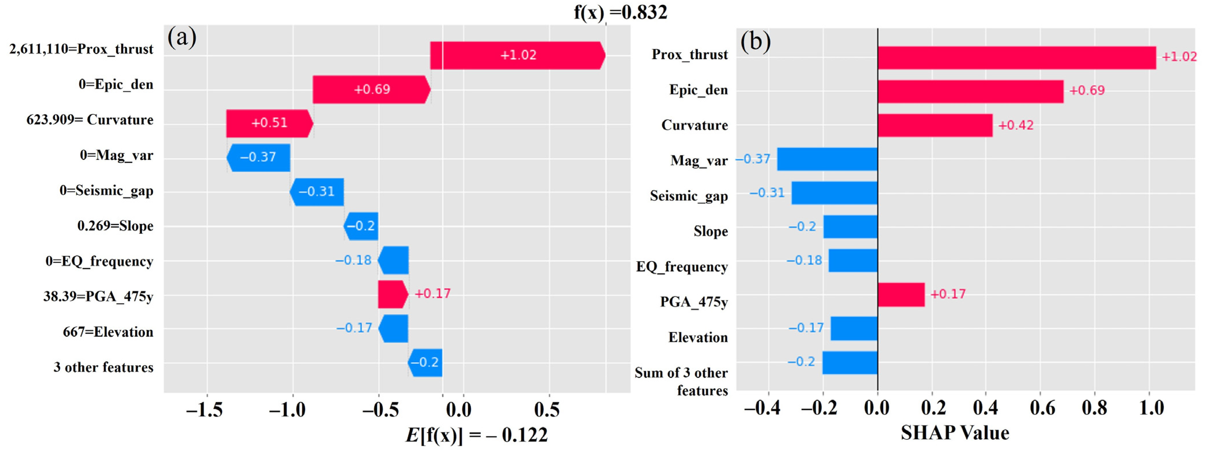
Waterfall plots are conceived to explain individual predictions (Figure 4a) and portray a single row of the whole data as input (Figure 4b). The bottom of a waterfall plot shows the expected model output. The positive (red) or negative (blue) contribution in each row shows the value that moves from the expected model output to the model output in each prediction. Figure 4 shows the plots for the first explanation of Inception v3-XGBoost based on the waterfall plot. The log-odds units are presented on the x-axis, so negative values denote the probabilities of less than 0.5.
The gray text behind the factors shows the value of each factor for the individual sample. Interestingly, having proximity to a thrust of 2,611,110 m dramatically increases the predicted spatial probability of earthquakes. Seeing that the waterfall plots only manifest a single row worth of data makes it hard to understand the impact of changing values of the factor proximity to thrust. To demonstrate this, a scatter plot is necessary to show that low SHAP values are the negative predictor of earthquakes, while high values are the positive predictor (Figure 5a–d). To explain the result, a deep dive into the data is required and careful training of the model is necessary with bootstrap resamples for uncertainty quantification. The important factors as per the waterfall plot were considered for scatter plotting of SHAP values. The SHAP values are clustered against their original factor values. In the case of non-earthquake prediction, proximity to thrust, epicenter density, curvature, and magnitude variation, the values vary from 0 to −1.8, 0 to −1.5, 0 to −1.6, and 0 to −4, respectively. Similarly, for earthquake prediction, proximity to thrust, epicenter density, curvature, and magnitude variation, the values vary from 0 to 1.6, 0 to 2.5, 0 to 1.7, and 0 to 5, respectively.
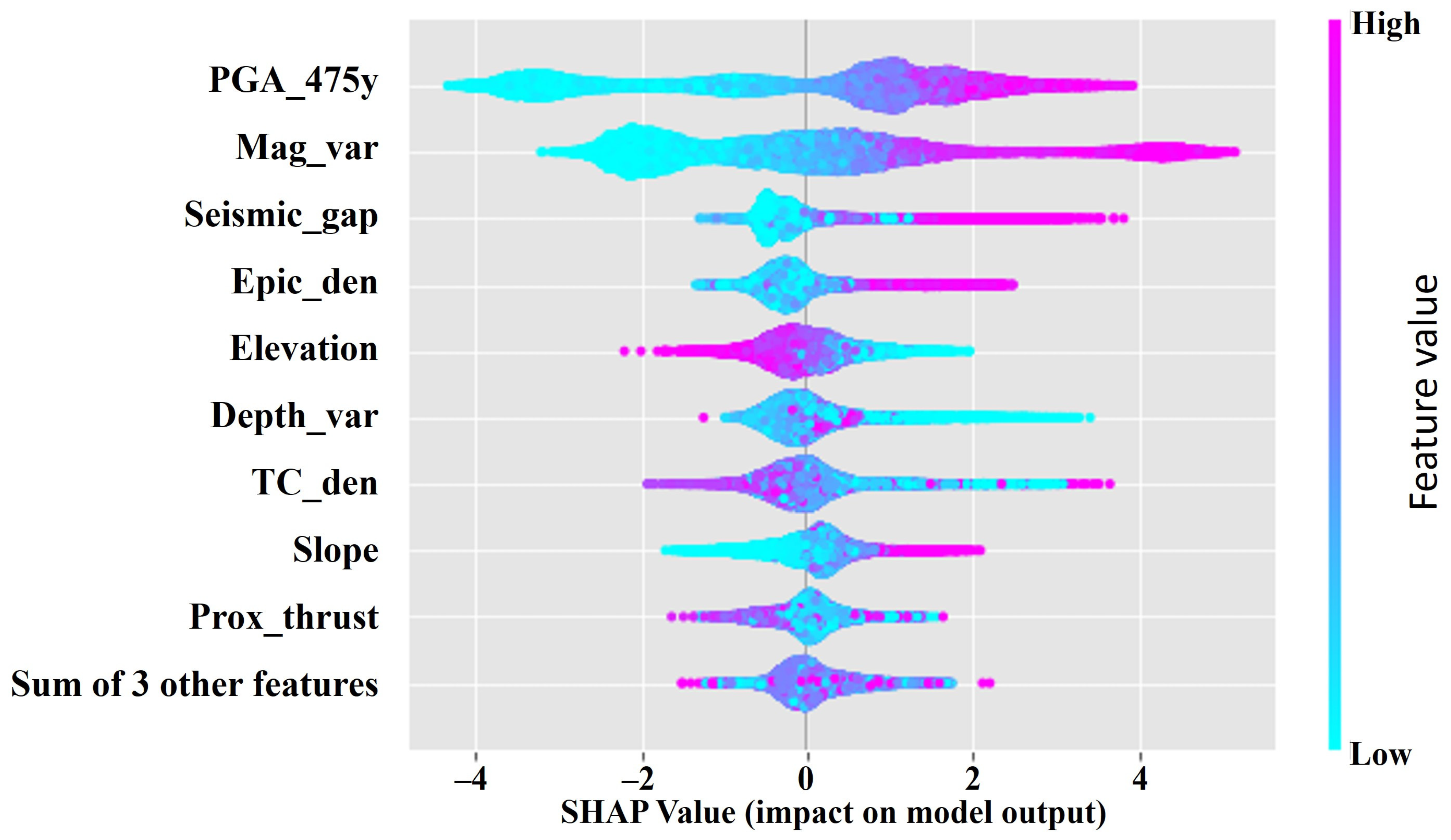
According to the factor’s importance in the earthquake SPA, Figure 6a shows the variation of SHAP values. As per the results, PGA and magnitude variation contribute the highest with the SHAP values of 4.3 and 5, respectively. All other factors are contributing the highest, with SHAP values ranging from 0 to 0.7. Figure 6b represents the bar diagram showing the mean SHAP values in SPA, where the highest value is achieved by PGA and magnitude variation, respectively. Lower SHAP values were observed for the factors such as earthquake frequency, curvature, and sand-filled geology, which contribute to a minimal level of earthquake SPA.
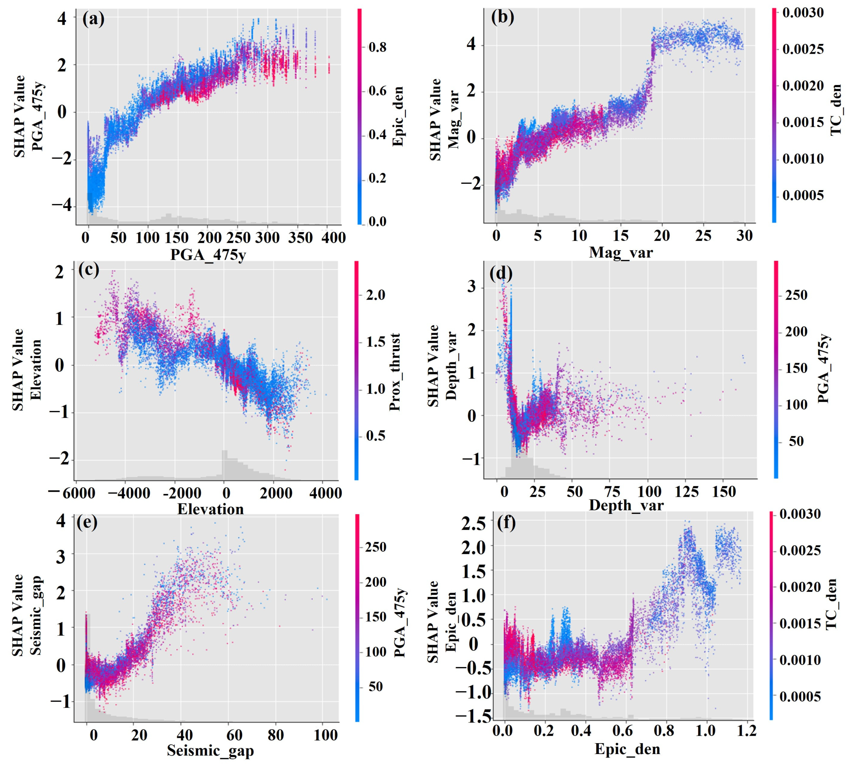
The hybrid model performed well in classifying earthquakes and non-earthquake points by detecting earthquake points. However, it failed to detect some of the earthquake and non-earthquakes points in the test dataset. A possible reason behind the high number of true-negative results could be due to the skewed dataset towards the non-earthquake points. The accuracy is below 90% because the model predicts more non-earthquake points. Individually, the SHAP values for earthquakes and non-earthquakes are plotted in red and blue color in a scatter plot, respectively (Figure 7a–f). This will overcome the issue of visualization observed in a simple scatterplot. In the SHAP colored scatter plot, the colors such as blue, purple, and red color denote the low, average, and high values of factors in the training dataset, respectively. The SHAP values in the Y-axis show each observation, while the X-axis shows the factor values. It is therefore necessary to create a summary plot in order to gain a better understanding of this concept. However, this plot is unable to describe when some low SHAP values are predicting earthquake points. Therefore, a summary plot is necessary to understand this concept.
The factors’ importance is shown in the SHAP summary plot (Figure 8). The seismological factors are portrayed as most impactful in distinguishing the earthquake points and non-earthquake points. This result is obvious because the PGA, magnitude, epicenter, and depth variation are the properties that define earthquake probability areas. In contrast, some factors do not have a significant effect on model predictions. The low contribution of the factors in the classification might be controlled by zero values in most of the data points. Therefore, due to the low variance in the factors does not provide sufficient information to contribute to the classification, which is evident in the SHAP summary plot (Figure 8). In the SHAP summary plot, the aqua blue, purple, and fuchsia red colors denote the low, average, and high SHAP values of factors, respectively. The SHAP values in the X-axis show each observation. Therefore, the interaction between the factors and the target can be explored using this plot. Moreover, most of the earthquake points occurred in the potential areas according to the previously published maps of Al-Haddad et al. [19,20]. Therefore, a correlation might be observed between low-important factors in the study area and its condition with the earthquake spatial probability. However, this study found these factors are irrelevant and can be removed from the dataset. Further, due to low contribution in SPA estimation curvature, earthquake frequency, and geology are likely to be redundant. It was found that geology is not important as the entire peninsula is characterized by dried sands. For PGA and magnitude variation, the SHAP values are highest and vary from −4.5 to 4 and −3.5 to 4.5, while for SPA, the values vary from 0 to 4 and 0 to 4.5, respectively. The study will provide new results if the irrelevant and redundant factors are removed. The nine remaining seismological and structural factors can lead to good accuracy; however, the accuracy will go down. The SHAP values for all factors were calculated and presented in Figure 8. It can be expected that the new SHAP summary results will portray seismological factors as the most important factors for SPA estimation.
If the attributes correlation is perfectly positive or negative, then there is a high chance that the model performance will be impacted by “Multicollinearity”. In fact, Multicollinearity occurs when one predictor in a multiple regression model can be predicted from others in a linear manner having a high degree of accuracy. Therefore, this can lead to skewed or misleading results.

4.2. Spatial and Temporal Probability Assessment

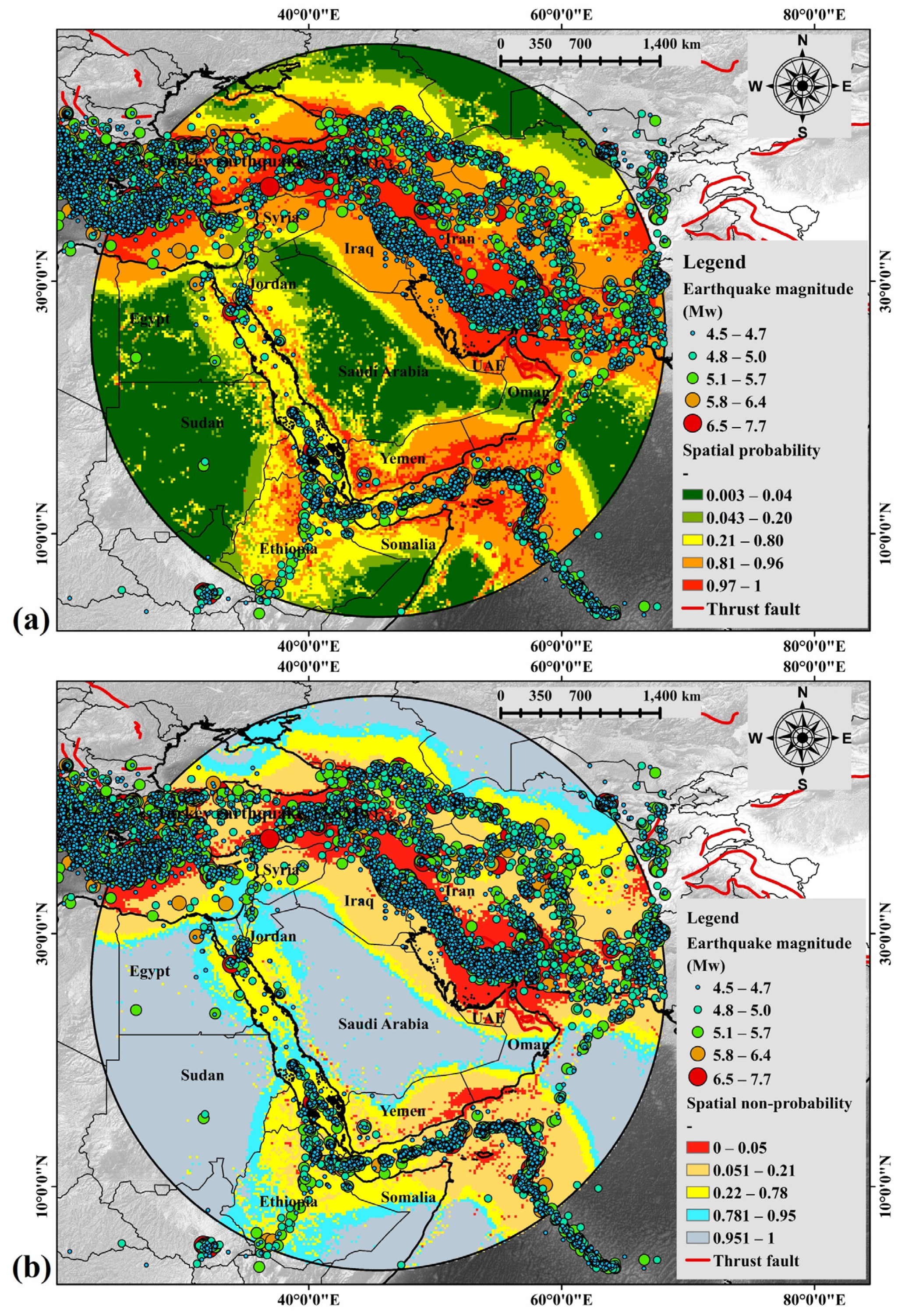
The earthquake spatial probability (Figure 9a) and non-spatial probability (Figure 9b) maps are presented. Based on the probabilistic point of view, the index varies between 0 (non-earthquakes) and 1 (earthquakes) derived using SoftMax and classified based on the natural break’s classification technique. The classified values can be compared for different locations which can, later, be used for the hazard assessment based on seismic coding and retrofitting. The probability index was classified into five different classes such as 0.002–0.01 (very low), 0.011–0.093 (low), 0.094–0.91 (medium), 0.92–0.99 (high), and 0.991–1 (very high).
The index values in the non-probability map were classified into five different classes such as 0–0.01 (very low), 0.012–0.11 (low), 0.12–0.89 (medium), 0.89–0.98 (high), and 0.99–1 (very high). Most of the high to very high spatial probability zones are characterized by more than 5.5 Mw events. A comparison between the probability maps without (Figure 10a) and with 3 important factors was conducted. The result shows that the one with 3 important factors portrays better output than the one without PGA, magnitude variation, and seismic gap as shown below. Unrealistic and poor results can be seen in Figure 10b, which portrays a vast region of the Arabian Peninsula that falls under a high probability zone.
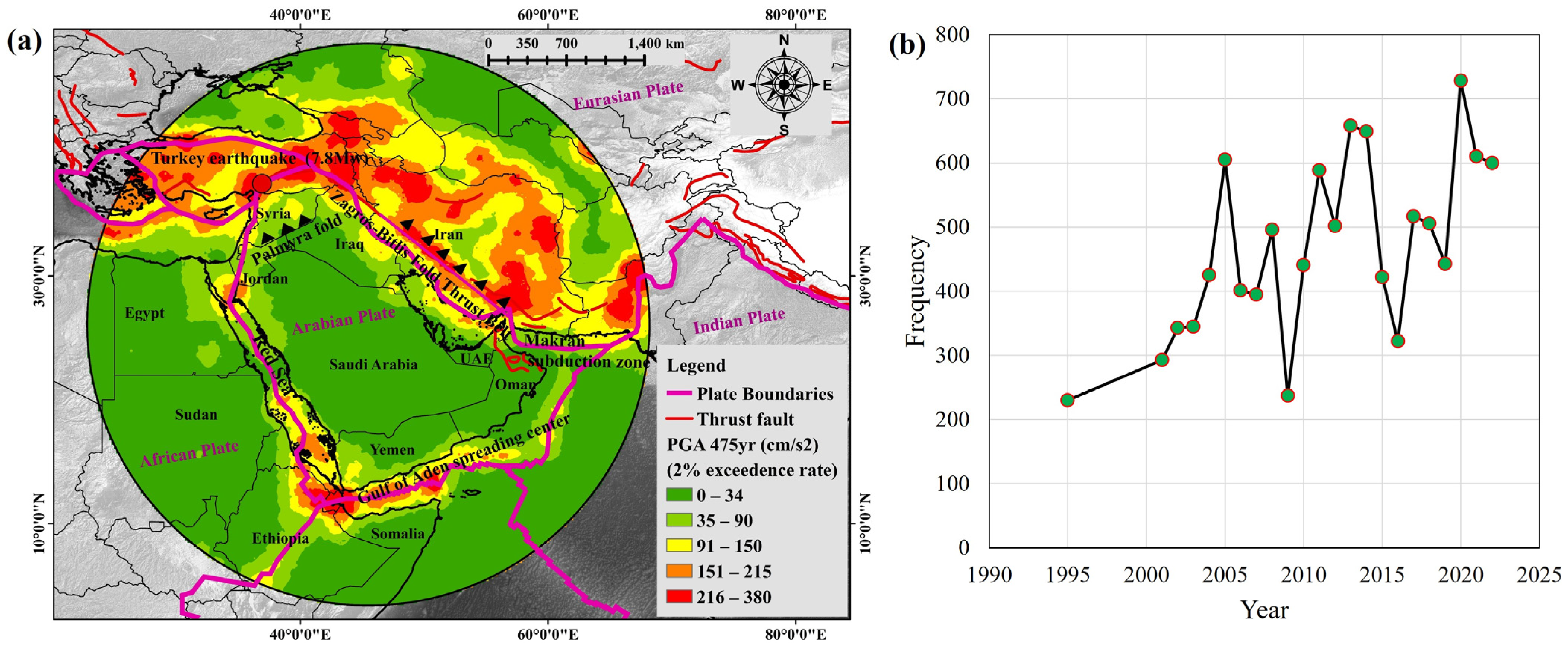
For a return period of 475 years., the PGA was estimated (Figure 11a) based on the PSHA technique for the Arabian Peninsula where, eastern parts of UAE, and Iraq, northwestern parts of Syria and Jordan, and southwestern parts of Yemen are falling under a medium range of PGA values (91–150 cm/s2). The current earthquake in Turkey is falling under a very high PGA value ranging from (216–380 cm/s2) causing the location highly hazardous. The frequency vs. time shows that frequency has increased significantly from 1995 onwards and reached 600 events in 2023 (Figure 11b).

4.3. Validation and Threshold Evaluation

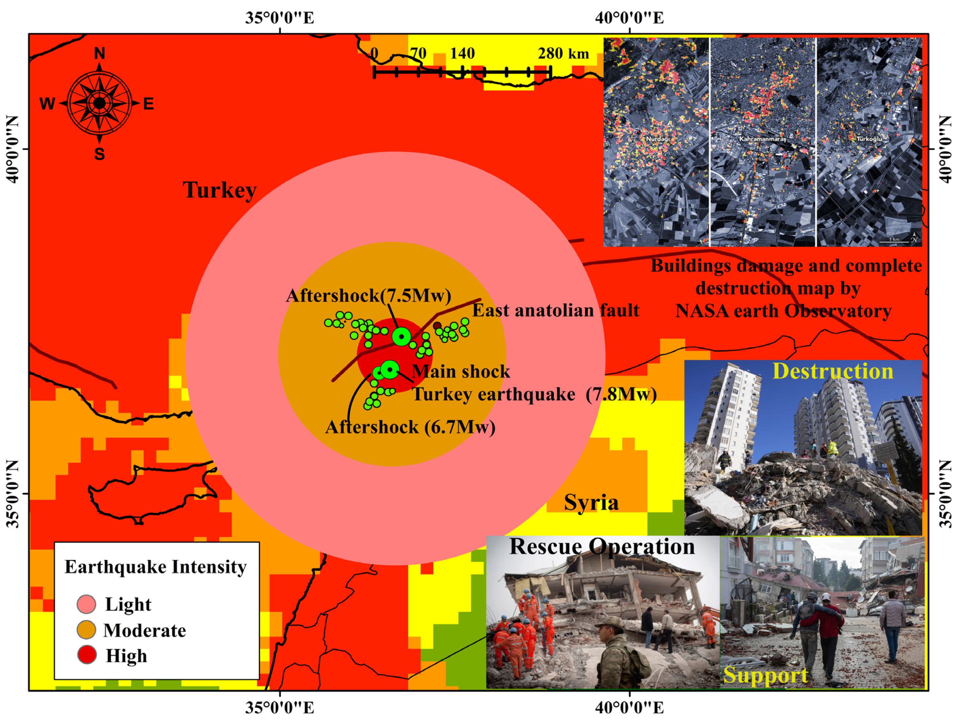
Validation of the obtained results of earthquake SPA (Figure 10) and PGA (Figure 11) using the recent main and aftershock earthquakes in Turkey was conducted. The recent Turkey events of Mw 7.8, Mw 7.5, and Mw 6.7 may be falling within or very close to a seismic gap in Turkey. The events are falling under the spatial probability index values of (0.991–1) based on the Inception v3-XGBoost model with all major factors. Similarly, the events are falling within a high PGA (216–380 cm/s2) zone confirming the accuracy of the obtained result. These events including more than 45 aftershocks caused huge destruction. Threshold for all the factors and their weighted score were derived (Table 4).
According to the Inceptionv3-XGBoost model, the highest weights were achieved by PGA (14%), magnitude variation (13%), seismic gap (12%), and epicenter density (10%). These are the four highly recommended and globally stable factors for the SPA in the Arabian Peninsula. The threshold achieved for all these four factors are >100 cm/s2, >Mw 5.5, >500 km, and >8 events in a cluster, respectively.

4.4. Model Performance Evaluation

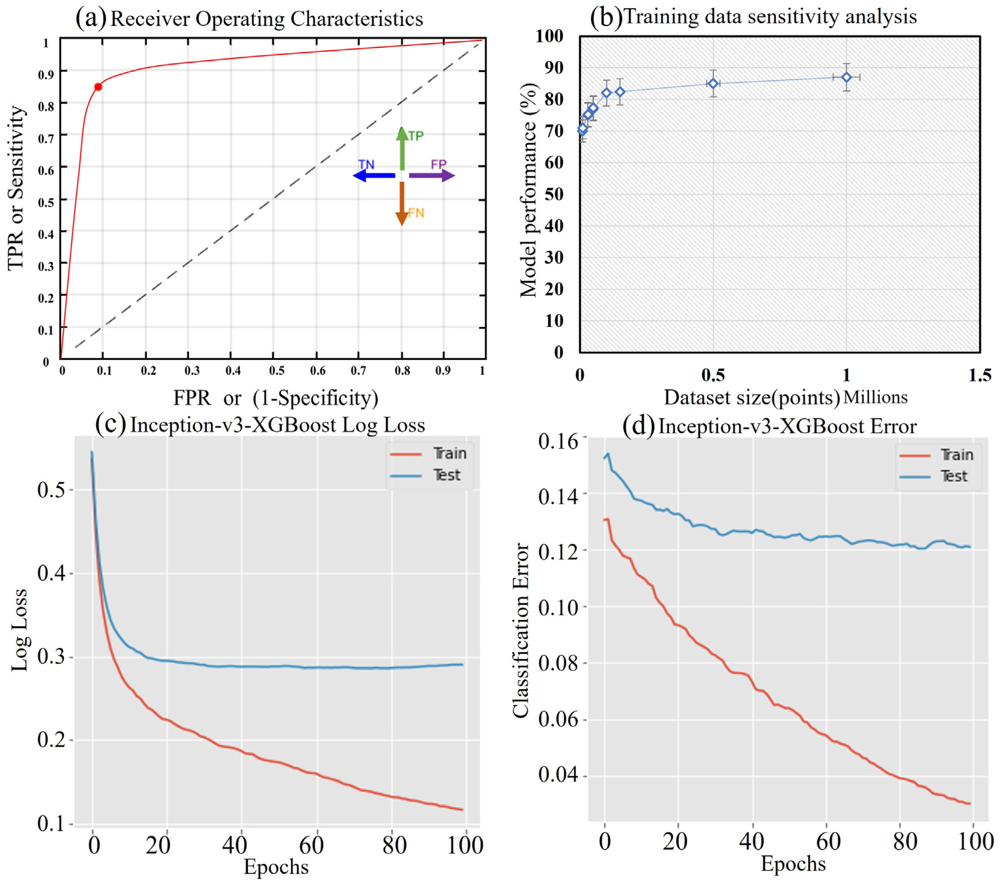
A confusion matrix and classification report were derived to measure the model performance, as presented in Table 5 and Table 6, respectively. A total of 12,000 points were considered for training and validation purposes, out of which 6000 points were trained as earthquake points. A total of 6000 random points were considered for non-earthquakes training purposes. The receiver operating characteristics (ROC) curve was plotted as shown in Figure 12a which shows the accuracy (87.9%) of the proposed model. The sensitivity assessment for the employed training data was conducted which shows that with an increase in the training data points, the accuracy increases. For a minimum of 10,000 data points the accuracy reaches up to 70% whereas the accuracy gradually increases until 1,000,000 points (Figure 12b).
After the pre-processing stage, 1,000,000 points were derived from the study area for testing purposes. The hybrid model achieved an overall accuracy of 87.91%. The macro average was achieved by the model with a precision of 0.8805, while the weighted average with a precision of 0.8806. The earthquake probability classification achieved a precision of 0.8557, while the earthquake non-probability assessment achieved a precision of 0.9053. This shows that the trained model classifies the non-earthquake points more efficiently than earthquake points. The predicted probability against log loss (Figure 12c) and classification error is shown in Figure 12d.

5. Discussion

In the current study, the SPA was conducted in Arabian Peninsula using a combined approach of ML and XAI techniques. Because feature learning is still unclear in the literature, therefore a hybrid combination of the Inception v3-XGBoost model was developed for clarity. This hybrid model performs both feature learning and prediction better than the standalone models [50]. The model deeply analyses the features to improve processes, automate tasks, and predict outcomes, based on past experiences. Several instance-level plots for the explanations can be very informative [56]. To interpret the effect of the feature on the prediction, waterfall, scatter, bar, and summary plots were plotted. This investigates the factors’ impact on earthquake and non-earthquake classification (Figure 5, Figure 6, Figure 7, Figure 8 and Figure 9). As shown in Figure 9, the trained XGBoost model could correctly classify the earthquake and non-earthquake areas, respectively.
The way of summarizing the importance of factors can make a big difference in understanding the model. In the plot shown in Figure 8, the topmost factors can be seen, which portrays the impact and common interaction. The study uses the SHAP model to summarize the factor’s importance and the largest impact on the model. It can be noted that the high-rank factors lead to an increase in SHAP values. However, the increase in the low-rank factors leads to a decrease in SHAP values. It is worth noting that the results portray the general factors analysis in the dataset, and the factors might impact the classification output differently for individual events.
When estimating earthquake SPA using ML, the SHAP plots can help in understanding the reasons behind the specific model outputs. Somala et al. [57] conducted a study on the time period estimation of reinforced concrete (RC) frames. They successfully estimated the SHAP values of the input parameters and their importance. Matin et al. [58] conducted a study on earthquake-induced building-damage mapping using explainable AI. This paper successfully implemented SHAP to interpret the outputs of the proposed ANN model and analyzed the impact of the feature to understand the model’s reliability. Though, it would be precipitous to fully believe SHAP that can explain the contribution of the factors, as currently, no literature is available on earthquake SPA using SHAP. Nevertheless, with an increase in studies on hazard estimation, researchers could trust SHAP to understand the importance of the factors on SPA estimation.
This study conducted an assessment by removing the low-impact factors to see the changes in results. The results after removing the low-impact factors do not provide any remarkable changes in the outputs. Therefore, the presence or absence of low-impact factors does not matter to the model. However, the spatial variation of factors after removing the low contribution factors of specific predictors does not show any changes in ranking. This could be due to the reduction of the test dataset. Then another assessment was conducted by removing the high-influence factors, as shown in Figure 10. Looking at the spatial variation, some differences could be observed in both maps (Figure 10). The important point is that the SHAP algorithm was not developed for time series analysis, with the development of deepExplainer still situated in its incipient stage [59]. As per the current analysis, deepExplainer suits the proposed model. Individual rows of data and their contribution were compared based on explainers which show a minimum distance of 0.33 and a maximum of 0.48. SHAP values, however, can provide valuable information that is correlated with the results of actual predictions. Therefore, this could lead to explaining in detail the black box models for all stages of analysis in the future.
The results of the current study considered the postulation that future events might fall within the mapped seismic zones. This might not happen as few areas in the peninsula have shown seismic quiescence for a long period. These are the Makran Subduction Zone and the Gulf of Aqaba, which may become active in the future. This confirms further studying the active tectonics in the Peninsula and surrounding areas. The earthquake inventory indicates strong shaking at Nizwa, Qalhat, Najran, Sohar, Makah, Al-Madinah, Taief, and Tabuk manifesting significant seismic probability and hazard warnings within the Arabian Plate. However, most of the recorded earthquakes suggest that the Arabian Plate is aseismic [20]. The SPA is tied to some specific faults in Iran and Turkey rather than an average area, indicating accurate and localized spatial probability. Therefore, state-of-the-art AI-based studies on paleo-seismicity and active faulting in association with field investigations could confirm or deny the historical reports. This research implemented the seismic gap as a new factor, which comes as the third most important factor in the SPA analysis. The spatial seismic probability areas of the current study are similar to the map produced by Al-Haddad et al. [20].
As this study predicted the SPA based on binary classification techniques, therefore, the probability values vary between 0 (non-earthquake) and 1 (earthquake). The obtained SPA is comparable to some extent with the PGA map derived by Al-Haddad et al. [20] which shows high PGA with a ground motion of 250 cm/s2 in the southwestern part of Saudi Arabia. A little difference in mapped areas could be observed which are because of several reasons: (1) the current study implemented an updated catalog and recent GMPEs for PGA estimation, (2) the current work contemplates Iran and Southeastern Turkey as seismic sources, (3) adopted hybrid machine learning model (Inception v3-XGBoost), and (4) inclusion of new input parameters and treated the factors appropriately. Generally, the SPA in the current study is consistent with the earthquake events showing Central Saudi Arabia, Egypt, and Sudan come under low probability levels (index values range from 0.002 to 0.093). Medium-to-high probability index ranges from 0.94 to 0.99 surrounding the very high probability areas. Very high probability index (falling under the index values ranging from 0.991 to 1) can be found in the Gulf of Aden, Red Sea, Iran, and Turkey (Figure 13). The current study, therefore, may convey the hybrid ML-based SPA improves the previous works in the Arabian Peninsula [3,19,20] as shown in (Figure 9). This work is limited to SPA estimation without any risk assessment. A large area of study needs a huge amount of training data for better accuracy. This can be studied using smart predictors to improve the SPA map. The proposed hybrid Inception V3-XGBoost model achieved good accuracy as compared to other state-of-the-art ML models. However, the CNN model achieved a better accuracy in prediction which is 90%. Detailed information about the achieved accuracy by several ML models is shown in Table 7.

6. Conclusions

Earthquakes spatial probability assessment is the most challenging among all natural hazards owing to multiple factors and event non-linearity. The transparency and explainability of the AI-based models in the field of earthquake SPA were aimed in this work. The advantages of the current study deal with operationalizing AI that builds confidence in black-box models and monitors the models to optimize. Because this is the first ever study using XAI for SPA, the main findings of the work are as follows:
The hybrid Inception v3-Ensemble XGBoost model was found to be an effective and robust approach for SPA and its global acceptability should be further tested with new factors and geotectonic conditions.
The SHAP implementation builds more trust toward the implementation of ML models, thereby grasping data-mining models for SPA.
The study found the importance of the seismic gap as a predictor in SPA along with eight other factors confirming its insertion in the assessment.
The results show that Central Saudi Arabia, Egypt, and Sudan come under low probability levels (index values range from 0.002 to 0.093) dominating the major parts of the Arabian Peninsula. Very high probability index (falling under the index values ranging from 0.991 to 1) can be found in the Gulf of Aden, Red Sea, Iran, and Turkey.
The recent earthquake of Mw 7.8 and the corresponding aftershocks show the importance of this study and can be used to validate the obtained results.
This may substantially contribute to establishing seismic codes for buildings in the Arab’s pioneering project. Further, the results could provide relevant parameters to determine whether retrofitting is necessary to minimize ground-shaking effects in the Arabian Peninsula.
In earthquake SPA work, the inclusion of subduction-related parameters, fault surface area, and fault width is necessary for a better representation of seismic coupling and probability estimation.
Future works should include SHAP, Local Interpretable Model-Agnostic Explanations (LIME), and extreme deep learning models for long lead time–magnitude prediction in association with integrated earthquake research.

Author Contributions

Conceptualization, R.J., A.S. and R.A.-R.; methodology, R.J., A.S., R.A.-R. and M.B.A.G.; software, R.J.; validation, R.J., A.S. and R.A.-R.; formal analysis, R.J., O.G., A.S. and R.A.-R.; investigation, A.S.; resources, A.S.; data curation, R.A.-R.; writing—original draft preparation, R.J.; writing—review and editing, R.J., A.S., R.A.-R., B.P., M.B.A.G., M.A.K., O.G., G.P.G. and P.G.; visualization, R.J., A.S., R.A.-R. and B.P.; supervision, A.S. and R.A.-R.; project administration, A.S.; funding acquisition, A.S., R.A.-R., O.G. and P.G. All authors have read and agreed to the published version of the manuscript.

Funding

The work was supported by the GIS and Remote Sensing Center, Research Institute of Sciences and Engineering, University of Sharjah, UAE through the Vice Chancellor Research Fund and the APC was funded by the Institute of Advanced Research in Artificial Intelligence (IARAI) GmbH, Vienna, Austria.

Data Availability Statement

The data that support the findings of this study are available from the corresponding author, [R.J.], upon reasonable request.

Conflicts of Interest

The authors declare no conflict of interest.

References

  1. Yanilmaz, S.; Baskak, D.; Yucesan, M.; Gul, M. Extension of FEMA and SMUG Models with Bayesian Best-Worst Method for Disaster Risk Reduction. Int. J. Disaster Risk Reduct. 2021, 66, 102631. [Google Scholar] [CrossRef]
  2. USGS. USGS Science for a Changing World. 2022. Available online: https://www.usgs.gov/faqs/why-are-we-having-so-many-earthquakes-has-naturally-occurring-earthquake-activity-been (accessed on 18 November 2022).
  3. Pascucci, V.; Free, M.W.; Lubkowski, Z.A. Seismic Hazard and Seismic Design Requirements for the Arabian Peninsula Region. In Proceedings of the 14th World Conference on Earthquake Engineering, Beijing, China, 12–17 October 2008. [Google Scholar]
  4. Jackson, E.L. Response to Earthquake Hazard: The West Coast of North America. Environ. Behav. 1981, 13, 387–416. [Google Scholar] [CrossRef]
  5. Dowrick, D.J. Earthquake Risk Reduction; John Wiley & Sons: Hoboken, NJ, USA, 2003; ISBN 0470869348. [Google Scholar]
  6. Bommer, J.J. Deterministic vs. Probabilistic Seismic Hazard Assessment: An Exaggerated and Obstructive Dichotomy. J. Earthq. Eng. 2002, 6, 43–73. [Google Scholar] [CrossRef]
  7. Magrin, A.; Peresan, A.; Kronrod, T.; Vaccari, F.; Panza, G.F. Neo-Deterministic Seismic Hazard Assessment and Earthquake Occurrence Rate. Eng. Geol. 2017, 229, 95–109. [Google Scholar] [CrossRef]
  8. Hardebeck, J.L. Stress Triggering and Earthquake Probability Estimates. J. Geophys. Res. Solid Earth 2004, 109, B04310. [Google Scholar] [CrossRef]
  9. Parsons, T. Significance of Stress Transfer in Time-dependent Earthquake Probability Calculations. J. Geophys. Res. Solid Earth 2005, 110, B05S02. [Google Scholar] [CrossRef]
  10. Shcherbakov, R.; Zhuang, J.; Zöller, G.; Ogata, Y. Forecasting the Magnitude of the Largest Expected Earthquake. Nat. Commun. 2019, 10, 4051. [Google Scholar] [CrossRef] [PubMed]
  11. Schäfer, A.M.; Wenzel, F. Global Megathrust Earthquake Hazard—Maximum Magnitude Assessment Using Multi-Variate Machine Learning. Front. Earth Sci. 2019, 7, 136. [Google Scholar] [CrossRef]
  12. Gitis, V.G.; Derendyaev, A.B. Machine Learning Methods for Seismic Hazards Forecast. Geosciences 2019, 9, 308. [Google Scholar] [CrossRef]
  13. Jena, R.; Pradhan, B.; Al-Amri, A.; Lee, C.W.; Park, H. Earthquake Probability Assessment for the Indian Subcontinent Using Deep Learning. Sensors 2020, 20, 4369. [Google Scholar] [CrossRef]
  14. Jena, R.; Pradhan, B.; Naik, S.P.; Alamri, A.M. Earthquake Risk Assessment in NE India Using Deep Learning and Geospatial Analysis. Geosci. Front. 2021, 12, 101110. [Google Scholar] [CrossRef]
  15. Jena, R.; Pradhan, B.; Beydoun, G.; Sofyan, H.; Affan, M. Integrated Model for Earthquake Risk Assessment Using Neural Network and Analytic Hierarchy Process: Aceh Province, Indonesia. Geosci. Front. 2020, 11, 613–634. [Google Scholar] [CrossRef]
  16. Pourghasemi, H.R.; Gayen, A.; Panahi, M.; Rezaie, F.; Blaschke, T. Multi-Hazard Probability Assessment and Mapping in Iran. Sci. Total Environ. 2019, 692, 556–571. [Google Scholar] [CrossRef] [PubMed]
  17. Al-Haddad, M.; Siddiqi, G.H.; Al-Zaid, R.; Arafah, A.; Necioglu, A.; Turkelli, N. A Basis for Evaluation of Seismic Hazard and Design Criteria for Saudi Arabia. Earthq. Spectra 1994, 10, 231–258. [Google Scholar] [CrossRef]
  18. Al-Haddad, M.S.; Siddiqi, G.H. Seismic Design Recommendations for Building Structures in Saudi Arabia. J. King Saud Univ. Sci. 1995, 7, 25–44. [Google Scholar] [CrossRef]
  19. Allen, M.; Jackson, J.; Walker, R. Late Cenozoic Reorganization of the Arabia-Eurasia Collision and the Comparison of Short-term and Long-term Deformation Rates. Tectonics 2004, 23, TC2008. [Google Scholar] [CrossRef]
  20. Vernant, P.; Nilforoushan, F.; Hatzfeld, D.; Abbassi, M.R.; Vigny, C.; Masson, F.; Nankali, H.; Martinod, J.; Ashtiani, A.; Bayer, R. Present-Day Crustal Deformation and Plate Kinematics in the Middle East Constrained by GPS Measurements in Iran and Northern Oman. Geophys. J. Int. 2004, 157, 381–398. [Google Scholar] [CrossRef]
  21. Hessami, K.; Jamali, F.; Tabassi, H. Major Active Faults of Iran; IIEES: Tehran, Iran, 2003. [Google Scholar]
  22. Al-shijbi, Y.; El-Hussain, I.; Deif, A.; Al-Kalbani, A.; Mohamed, A.M.E. Probabilistic Seismic Hazard Assessment for the Arabian Peninsula. Pure Appl. Geophys. 2019, 176, 1503–1530. [Google Scholar] [CrossRef]
  23. Bulut, F.; Bohnhoff, M.; Eken, T.; Janssen, C.; Kılıç, T.; Dresen, G. The East Anatolian Fault Zone: Seismotectonic Setting and Spatiotemporal Characteristics of Seismicity Based on Precise Earthquake Locations. J. Geophys. Res. Solid Earth 2012, 117, 7304. [Google Scholar] [CrossRef]
  24. Aldama-Bustos, G.; Bommer, J.J.; Fenton, C.H.; Stafford, P.J. Probabilistic Seismic Hazard Analysis for Rock Sites in the Cities of Abu Dhabi, Dubai and Ra’s Al Khaymah, United Arab Emirates. Georisk 2009, 3, 1–29. [Google Scholar] [CrossRef]
  25. El-Hussain, I.; Deif, A.; Al-Jabri, K.; Toksoz, N.; El-Hady, S.; Al-Hashmi, S.; Al-Toubi, K.; Al-Shijbi, Y.; Al-Saifi, M.; Kuleli, S. Probabilistic Seismic Hazard Maps for the Sultanate of Oman. Nat. Hazards 2012, 64, 173–210. [Google Scholar] [CrossRef]
  26. Babiker, N.; Mula, A.H.G. A Unified Mw-Based Earthquake Catalogue and Seismic Source Zones for the Red Sea Region. J. Afr. Earth Sci. 2015, 109, 168–176. [Google Scholar] [CrossRef]
  27. Huijer, C.; Harajli, M.; Sadek, S. Re-Evaluation and Updating of the Seismic Hazard of Lebanon. J. Seismol. 2016, 20, 233–250. [Google Scholar] [CrossRef]
  28. Coleman, R.G. Geologic Evolution of the Red Sea (Oxford Monographs on Geology and Geophysics, 24); Oxford University Press: New York, NY, USA, 1993; p. 186. [Google Scholar]
  29. Khan, M.; Ali, M. Optimization of Concrete Stiffeners for Confined Brick Masonry Structures. J. Build. Eng. 2020, 32, 101689. [Google Scholar] [CrossRef]
  30. Khan, M.; Lao, J.; Dai, J.-G. Comparative Study of Advanced Computational Techniques for Estimating the Compressive Strength of UHPC. J. Asian Concr. Fed. 2022, 8, 51–68. [Google Scholar] [CrossRef]
  31. Chakraborty, A.; Sivaram, A.; Venkatasubramanian, V. AI-DARWIN: A First Principles-Based Model Discovery Engine Using Machine Learning. Comput. Chem. Eng. 2021, 154, 107470. [Google Scholar] [CrossRef]
  32. Irwandi, I. Advantages of Realistic Model Based on Computational Method: NDSHA versus Standard PSHA. In Proceedings of the IOP Conference Series: Earth and Environmental Science, Shanghai, China, 19–22 October 2017; IOP Publishing: Shanghai, China, 2017; Volume 56, p. 12007. [Google Scholar]
  33. Shapley, L.S. Stochastic Games. Proc. Natl. Acad. Sci. USA 1953, 39, 1095–1100. [Google Scholar] [CrossRef]
  34. Schlegel, U.; Arnout, H.; El-Assady, M.; Oelke, D.; Keim, D.A. Towards a Rigorous Evaluation of Xai Methods on Time Series. In Proceedings of the 2019 IEEE/CVF International Conference on Computer Vision Workshop (ICCVW), Seoul, Republic of Korea, 27–28 October 2019; pp. 4197–4201. [Google Scholar]
  35. Deif, A.; Al-Shijbi, Y.; El-Hussain, I.; Ezzelarab, M.; Mohamed, A.M.E. Compiling an Earthquake Catalogue for the Arabian Plate, Western Asia. J. Asian Earth Sci. 2017, 147, 345–357. [Google Scholar] [CrossRef]
  36. Farhoudi, G.; Karig, D.E. Makran of Iran and Pakistan as an Active Arc System. Geology 1977, 5, 664–668. [Google Scholar] [CrossRef]
  37. Beyer, K.; Bommer, J.J. Relationships between Median Values and between Aleatory Variabilities for Different Definitions of the Horizontal Component of Motion. Bull. Seismol. Soc. Am. 2006, 96, 1512–1522. [Google Scholar] [CrossRef]
  38. Fenton, C.H.; Adams, J.; Halchuk, S. Seismic Hazards Assessment for Radioactive Waste Disposal Sites in Regions of Low Seismic Activity. Geotech. Geol. Eng. 2006, 24, 579–592. [Google Scholar] [CrossRef]
  39. ArRajehi, A.; McClusky, S.; Reilinger, R.; Daoud, M.; Alchalbi, A.; Ergintav, S.; Gomez, F.; Sholan, J.; Bou-Rabee, F.; Ogubazghi, G. Geodetic Constraints on Present-day Motion of the Arabian Plate: Implications for Red Sea and Gulf of Aden Rifting. Tectonics 2010, 29, TC3011. [Google Scholar] [CrossRef]
  40. Wason, H.R.; Das, R.; Sharma, M.L. Magnitude Conversion Problem Using General Orthogonal Regression. Geophys. J. Int. 2012, 190, 1091–1096. [Google Scholar] [CrossRef]
  41. Sakellariou, S.; Tampekis, S.; Samara, F.; Sfougaris, A.; Christopoulou, O. Review of State-of-the-Art Decision Support Systems (DSSs) for Prevention and Suppression of Forest Fires. J. For. Res. 2017, 28, 1107–1117. [Google Scholar] [CrossRef]
  42. Alizadeh, M.; Alizadeh, E.; Asadollahpour Kotenaee, S.; Shahabi, H.; Beiranvand Pour, A.; Panahi, M.; Bin Ahmad, B.; Saro, L. Social Vulnerability Assessment Using Artificial Neural Network (ANN) Model for Earthquake Hazard in Tabriz City, Iran. Sustainability 2018, 10, 3376. [Google Scholar] [CrossRef]
  43. Consultant, G. Final Report: Identification of Seismic Source’s Zone and Tsunami Hazard Probability as Considerations in Development Policy of Banda Aceh City; Nanggroe Aceh Darussalam Prov. (Package-1): Banda Aceh, Indonesia, 2009. [Google Scholar]
  44. Zebardast, E. Constructing a Social Vulnerability Index to Earthquake Hazards Using a Hybrid Factor Analysis and Analytic Network Process (F’ANP) Model. Nat. Hazards 2013, 65, 1331–1359. [Google Scholar] [CrossRef]
  45. Soe, M.; Ryutaro, T.; Ishiyama, D.; Takashima, I.; Charusiri, K.W.-I.P. Remote Sensing and GIS Based Approach for Earthquake Probability Map: A Case Study of the Northern Sagaing Fault Area, Myanmar. J. Geol. Soc. Thail 2009, 1, 29–46. [Google Scholar]
  46. Rashed, T.; Weeks, J. Assessing Vulnerability to Earthquake Hazards through Spatial Multicriteria Analysis of Urban Areas. Int. J. Geogr. Inf. Sci. 2003, 17, 547–576. [Google Scholar] [CrossRef]
  47. Dhar, S.; Rai, A.K.; Nayak, P. Estimation of Seismic Hazard in Odisha by Remote Sensing and GIS Techniques. Nat. Hazards 2017, 86, 695–709. [Google Scholar] [CrossRef]
  48. Alizadeh, M.; Ngah, I.; Hashim, M.; Pradhan, B.; Pour, A.B. A Hybrid Analytic Network Process and Artificial Neural Network (ANP-ANN) Model for Urban Earthquake Vulnerability Assessment. Remote Sens. 2018, 10, 975. [Google Scholar] [CrossRef]
  49. Kamranzad, F.; Memarian, H.; Zare, M. Earthquake Risk Assessment for Tehran, Iran. ISPRS Int. J. Geo-Inf. 2020, 9, 430. [Google Scholar] [CrossRef]
  50. Ramaneswaran, S.; Srinivasan, K.; Vincent, P.M.D.R.; Chang, C.-Y. Hybrid Inception v3 XGBoost Model for Acute Lymphoblastic Leukemia Classification. Comput. Math. Methods Med. 2021, 2021, 2577375. [Google Scholar] [CrossRef]
  51. Quinto, B. Introduction to Spark and Spark MLlib. In Next-Generation Machine Learning with Spark; Springer: Berlin/Heidelberg, Germany, 2020; pp. 29–96. [Google Scholar]
  52. Chen, T.; He, T.; Benesty, M.; Khotilovich, V.; Tang, Y.; Cho, H.; Chen, K.; Mitchell, R.; Cano, I.; Zhou, T.; et al. Xgboost: Extreme Gradient Boosting. R Packag. Version 0.6-4 2015, 1, 1–4. [Google Scholar]
  53. Li, H.; Cao, Y.; Li, S.; Zhao, J.; Sun, Y. XGBoost Model and Its Application to Personal Credit Evaluation. IEEE Intell. Syst. 2020, 35, 52–61. [Google Scholar] [CrossRef]
  54. Ma, J.; Yu, Z.; Qu, Y.; Xu, J.; Cao, Y. Application of the XGBoost Machine Learning Method in PM2. 5 Prediction: A Case Study of Shanghai. Aerosol Air Qual. Res. 2020, 20, 128–138. [Google Scholar] [CrossRef]
  55. Lundberg, S.M.; Lee, S.-I. A Unified Approach to Interpreting Model Predictions. In Proceedings of the 31st International Conference on Neural Information Processing Systems, Long Beach, CA, USA, 4–9 December 2017; Volume 30. [Google Scholar]
  56. Collaris, D.; Vink, L.M.; van Wijk, J.J. Instance-Level Explanations for Fraud Detection: A Case Study. arXiv 2018, arXiv:1806.07129. [Google Scholar]
  57. Somala, S.N.; Karthikeyan, K.; Mangalathu, S. Time Period Estimation of Masonry Infilled RC Frames Using Machine Learning Techniques. Structures 2021, 34, 1560–1566. [Google Scholar] [CrossRef]
  58. Matin, S.S.; Pradhan, B. Earthquake-Induced Building-Damage Mapping Using Explainable AI (XAI). Sensors 2021, 21, 4489. [Google Scholar] [CrossRef] [PubMed]
  59. Molnar, C. Interpretable Machine Learning; Lean Publishing: Victoria, BC, Canada, 2020; ISBN 0244768528. [Google Scholar]
  60. Asim, K.M.; Martínez-Álvarez, F.; Basit, A.; Iqbal, T. Earthquake Magnitude Prediction in Hindukush Region Using Machine Learning Techniques. Nat. Hazards 2017, 85, 471–486. [Google Scholar] [CrossRef]
  61. Huang, J.P.; Wang, X.A.; Zhao, Y.; Xin, C.; Xiang, H. Large Earthquake Magnitude Prediction in Taiwan Based on Deep Learning Neural Network. Neural Netw. World 2018, 28, 149–160. [Google Scholar] [CrossRef]
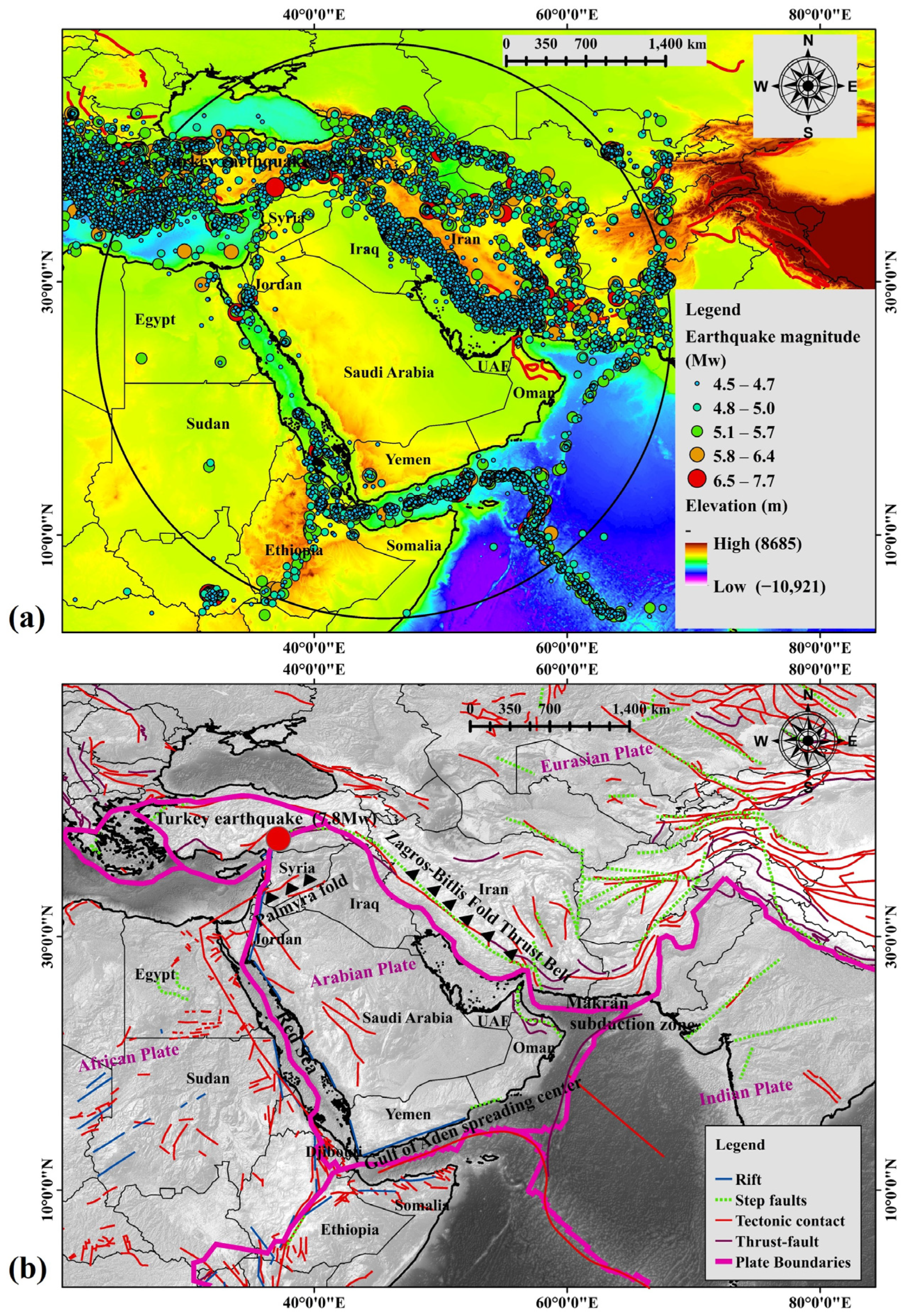
Figure 1. (a) Location of the study area. (The circle refers to the data collection area). (b) Different types of faults and tectonic boundaries along with the recent Turkey earthquake (Mw 7.8).
Remotesensing 15 02248 g001
Figure 2. Methodological flowchart for Inception v3-XGBoost based XAI interpretation for earthquake hazard estimation.
Remotesensing 15 02248 g002
Figure 3. Implementation of SHAP in model explanation followed by (a) Inception v3 and (b) XGBoost.
Remotesensing 15 02248 g003
Figure 4. (a) Waterfall plot shows the contribution of factors in an individual sample data, and (b) bar plot shows the contribution of the factors for earthquake and non-earthquake classification.
Remotesensing 15 02248 g004
Figure 5. The scatter plot shows SHAP values for important factors based on the waterfall plot; (a) proximity to thrust, (b) epicenter density, (c) curvature, and (d) magnitude variation.
Remotesensing 15 02248 g005
Figure 6. SHAP interpretation for earthquake SPA: (a) bee swarm plot portrays SHAP importance, and (b) bar plot shows importance based on mean SHAP values.
Remotesensing 15 02248 g006
Figure 7. Colored scatter plot with blue (0), purple (0.5), and red (1) possibilities. (a) PGA_475y, (b) Mag_var, (c) Elevation, (d) Depth_var, (e) Seismic_gap, (f) Epic_den.
Remotesensing 15 02248 g007
Figure 8. The summary plot shows the factors’ interaction and importance based on Inception v3-XGBoost model.
Remotesensing 15 02248 g008
Figure 9. SPA maps for Arabian Peninsula based on Inception v3-XGBoost model with PGA, magnitude variation, and seismic gap. (a) Spatial probability, (b) Spatial non-probability.
Remotesensing 15 02248 g009
Figure 10. SPA maps for Arabian Peninsula based on Inception v3-XGBoost model without PGA, magnitude variation, and seismic gap.
Remotesensing 15 02248 g010
Figure 11. (a) PGA map derived based on PSHA, and (b) earthquake frequency vs. year analysis.
Remotesensing 15 02248 g011
Figure 12. (a) ROC curve, (b) Sensitivity analysis for training, (c) XGBoost log loss, and (d) classification error for training and testing data.
Remotesensing 15 02248 g012
Figure 13. Recent main and aftershock earthquakes in Turkey are falling under the SPA maps based on Inception v3-XGBoost model causing huge destruction.
Remotesensing 15 02248 g013
Table 1. Earthquake characteristics, deaths, and injuries in Arabian Peninsula.
DateAreaMagnitudeIntensity (MMI)DeathsInjuriesRemarksSource
2009-05-19Madinah5.7 Mw 7LandslidesUSGS
2009-05-17Umm Lajj4.6 Mb DestructionUSGS
2004-06-09Tabuk Region4.6 ML Minor damageUSGS
1995-11-22Egypt, Saudi Arabia, Israel, Jordan7.3 MwVIII9–1230–69Moderate damage/tsunami
1072-03-16Yemen, Saudi Arabia VIII50 Moderate damageNGDC
1068-03-18Ramla, Jerusalem, Tabuk≥7.0IX~20,000 Destruction
551-07-09Lebanon, Egypt, Iraq, Saudi Arabia7.5 MwIX30,000+ Tsunami
Table 2. Data used in the current study.
Factors/30 m ResolutionInput PredictorsMethodsCode NameImportanceReferences
Earthquake inventoryMagnitudes > Mw 5
  • Earthquake inventory: experienced events used for training and testing purposes.
USGS, NEIC
Seismological
  • Slope (Degree)
  • Elevation (m)
  • Curvature (radians/m)
  • Magnitude variation (Mw)
  • Depth variation (m)
  • Epicenter density
  • Seismic gap (km)
  • Earthquake frequency
Machine learning (XGBoost)Slope
Elevation
Curvature
Mag_var
Dep_var
Epic_den
Seismic_gap
Eq_freq
  • Slope: controls the landscape processes and is associated with the crustal faults.
  • Elevation: complicated tectonics and earthquake probability vary with both high and low elevations.
  • Curvature: portrays the positive (ups) and negative (downs) of the surface.
  • Magnitude variation: probability of occurrence of a specific magnitude event at a particular location can be understood.
  • Depth variation: provides the source depth information on the fault zone.
  • Epicenter density: provides a view of the clusters of events. This locates in the high probable zone.
  • Seismic gap: stress accumulation occurs in the seismic gap which could lead to future mega-events.
  • Frequency: more the earthquake frequency, the less the magnitude of the event.
Sakellariou et al. [41]
Alizadeh et al. [42]
Gitamandalaksana [43].
Zebardast [44]
Soe et al. [45]
Rashed et al. [46]
Introduced factor
GeologicalGeologyExplainable AI (SHAP)Geology
  • Geology: amplification factors for soil and lithotypes are associated with grain size, compactness, and thickness.
Dhar et al. [47]
Geo-structural
  • Proximity to thrust faults (km)
  • Tectonic contacts density (km)
Prox_thrust
TC_den
  • Proximity to thrust faults: high magnitude earthquakes mostly occur on active thrust faults.
  • Tectonic contact density: most of the largest magnitude earthquakes happened in the region of tectonic contacts.
Alizadeh et al. [48]
Ground motionPGA (cm/s2)Probabilistic seismic hazard assessment using Joyner and Boore (1981) attenuation equations.PGA
  • PGA: provides ground acceleration information useful for hazard estimation.
Kamranzad et al. [49]
Table 3. Parameters used for the proposed model.
ParametersValues
Include_topTrue,
Weights“imagenet”,
Input_tensorNone,
Input shapeNone,
PoolingNone,
Boostergbtree
Verbosity1
Validate parametersTrue
n-threadMaximum
Disable default evaluation metricFalse
Number of p-bufferAutomatic
Number of featuresAutomatic
Adam Optimizer[0.9, 0.999]
Learning rate1 × 10−4
Table 4. Threshold and importance of factors derived based on Inception v3-XGBoost model.
FactorsClassImportance (%)ThresholdFactorsClassImportance (%)Threshold
Slope0–1.657>10Epicenter density0–210>8
1.65–4.952–4
4.95–9.904–6
9.90–17.606–8
17.60–70.148–10
Elevation−10,921–−40789>458Seismic gap0–19612>500 km
−4078–−1694196–392
−1694–458392–500
458–1995501–785
1995–8685785–981
Curvature−151,997–−45823<1479PGA0–3414>100 cm/s2
−4582–−147935–90
−1479–162491–150
1624–6279151–215
6279–243,695216–380
Magnitude variation4.5–5.513>5.5GeologyQuartz-rich sands5Quartz-rich sand and Oceanic crust with high amplification
5.5–5.8Oceanic crust
5.8–6.0Dry soil
6.0–6.38CaCO3
6.38–9.0Quartz-rich desert soil
Frequency0–25>6Proximity to thrust faults0–506.5<50 km
3–451–208
5–6208–385
6–7385–637
7–8637–999
Depth variation0–308<30 kmTectonic contacts density0–17.5>5
30–401–3
40–803–5
80–1205–7
120–1707–10
Table 5. Confusion matrix for Inception v3-XGBoost classification and statistical metrics.
Confusion Matrix:Predicted ConditionRMSER2
Actual conditionTotal populationPP (Positive)PN (Negative)0.350.52
P (Positive)2943527
N (Negative)3083126
Table 6. Classification report for Inception v3-XGBoost classification with macro and weighted average accuracy.
Classification Report:Predicted Condition
PrecisionRecallF1-ScoreSupport
00.90530.84810.87583470
10.85570.91030.88223434
Accuracy 0.87916904
Macro average0.88050.87920.87906904
Weighted average0.88060.87910.87906904
Classification accuracy: 0.879056; false discovery rate: 0.1519; Matthews correlation coefficient: 0.7597; sensitivity: 0.9053; specificity: 0.8557.
Table 7. Comparative assessment of Inception v3-XGBoost model with respect to state-of-the-art models. PRNN (primitives and recurrent neural network), RF (random forest), LPBoost (Linear programming boosting), ANN (artificial neural network), CNN (convolutional neural network).
ModelsAccuracyReferences
PRNN58%Asim et al. [60]
RNN64%
RF62%
LPBoost65%
ANN84%Jena et al. [15]
CNN90%Huang et al. [61]
Inceptionv3-XGBoost87.9%Proposed model
Disclaimer/Publisher’s Note: The statements, opinions and data contained in all publications are solely those of the individual author(s) and contributor(s) and not of MDPI and/or the editor(s). MDPI and/or the editor(s) disclaim responsibility for any injury to people or property resulting from any ideas, methods, instructions or products referred to in the content.