Article

Comparison of Different Remotely Sensed Data Sources for Detection of Presence of Standing Dead Trees Using a Tree-Based Approach

by
Marie-Claude Jutras-Perreault
*,
Terje Gobakken
,
Erik Næsset
and
Hans Ole Ørka
Faculty of Environmental Sciences and Natural Resource Management, Norwegian University of Life Sciences, NMBU, P.O. Box 5003, NO-1432 Ås, Norway
*
Author to whom correspondence should be addressed.
Remote Sens. 2023, 15(9), 2223; https://doi.org/10.3390/rs15092223
Submission received: 27 March 2023 / Revised: 12 April 2023 / Accepted: 20 April 2023 / Published: 22 April 2023

Abstract

:
Deadwood is an important key ecological element for forest ecosystem biodiversity. Its low occurrence, especially in managed forests, makes inventory through field campaigns challenging. Remote sensing can provide a more objective and systematic approach to detect deadwood for large areas. Traditional area-based approaches have, however, shown limitations when it comes to predicting rare objects such as standing dead trees (SDT). To overcome this limitation, this study proposes a tree-based approach that uses a local maxima function to identify trees from airborne laser scanning (ALS) and optical data, and predict their status, i.e., living or dead, from normalized difference vegetation index (NDVI). NDVI was calculated from aerial images (hyperspectral and simulated aerial image) and from satellite images (PlanetScope and Sentinel-2). By comparing the different remotely sensed data sources, we aimed to assess the impact of spatial and spectral resolutions in the prediction of SDT. The presence/absence of SDT was perfectly predicted by combining trees identified using ALS-derived canopy height models with spatial resolutions between 0.75 m and 1 m and a search window size of 3 pixels, and NDVI computed from aerial images to predict their status. The presence/absence of SDT was not predicted as accurately when using NDVI computed from satellite images. A root-mean-square deviation of around 35 trees ha−1 was obtained when predicting the density of SDT with NDVI from aerial images and around 60 trees ha−1 with NDVI from satellite images. The tree-based approach presented in this study shows great potential to predict the presence of SDT over large areas.

Graphical Abstract

1. Introduction

Forest ecosystem services are recognized to be critically important to human well-being and economic prosperity [1]. However, undervaluation of services with a less direct monetary value in decision-making has led to the degradation of forest ecosystem condition and the loss in biodiversity, threatening the capacity of forest ecosystems to deliver services [2]. The presence of deadwood is a key ecological factor for biodiversity [3,4,5,6]. Many saproxylic species that depend on decaying and dead trees for habitat are rare, threatened, or red-listed [4,7,8,9]. Deadwood is an important structural component of forest ecosystems [3,4,7,10,11,12] that provides a long-term source of organic matter and nutrients, increases site productivity, contributes to carbon sequestration, and controls soil erosion [3,7,10]. Thus, several forest management strategies in Europe include deadwood for monitoring biodiversity and forest condition [6].
After centuries of forest exploitation, very few forests unaffected by human activity remain in northern Europe [13]. In Fennoscandian countries, a large proportion of the forests are commercially managed [14]. Managed forests are consequently valuable habitats for many species and play a central role in the conservation of biodiversity [15,16,17]. To improve the management of biological diversity in forests, many northern European countries have adopted regulations concerning the preservation of woodland key habitats, i.e., small habitat patches identified as particularly valuable for maintaining landscape-level biodiversity [14]. In Norway, the authorities have implemented a habitat inventory approach called Complementary Hotspot Inventory (CHI), where habitats presenting specific qualities associated with high biodiversity and considered vulnerable to impact from forest operations are registered [18]. The registration of key habitats is implemented in Norwegian forestry through the certification process. Therefore, forest owners must take the appropriate measures to register key habitats to be set aside and preserved on the property to be able to sell certified timber [19]. Standing dead trees (SDT) is one of the 12 key habitats identified as crucial for the protection and valorization of biodiversity in forest ecosystems in Norway [13,20].
Identification of key habitats through CHIs is currently based on field surveys. Such field surveys are time-consuming and expensive and may be susceptible to errors due to the subjective assessments by the surveyors [21,22]. Delineation of the key habitats in the field can also be inaccurate due to decreased GPS accuracy under dense canopies [23]. Thus, tools or pre-information to guide the surveyors in finding and delineating key habitats more efficiently are needed to reduce cost and increase data quality.
Remotely sensed (RS) data have the potential to provide an objective and systematic approach to perform a wall-to-wall identification of SDT at a lower cost. In operational management inventories, area-based approaches are commonly used to estimate forest attributes such as heights and volume at stand level based on the relationship between field plot measurements or estimates, and plot-level metrics derived from RS data [24,25,26,27,28]. Area-based approaches were successfully used to detect SDT in conservation areas and in managed forests with large density of snags [29,30,31]. However, managed forests are more often characterized by a small occurrence of SDT, presenting a challenge in sampling enough SDT to build reliable area-based models. An unbalanced dataset can indeed lead to misclassification and inflated values of the estimates [32,33]. A study by [34] concluded that, in presence of an insufficient number of SDT sampled in the field reference data, a tree-based approach was more performant and more reliable than an area-based approach to detect the presence of SDT. With a tree-based approach, individual trees can be located using airborne laser scanning (ALS) point clouds [35,36], ALS-based canopy height models (CHM) [37,38,39], or with high spatial resolution optical images [40].
A popular technique to detect individual trees using ALS-derived CHMs or optical images is by using a local maxima algorithm. The local maxima methods assume that local maxima heights or high local intensities represent treetops, or apex of trees [41]. A local maximum is identified as the tallest or brightest pixel within a search window. A window size too small leads to the identification of nonexistent trees, crown edges or other features, while a window size too large results in a large omission error rate [42]. As ALS data provide three-dimensional characterizations of the forest structure [43], it is also possible to identify individual trees directly on the point cloud. Individual snags were identified using a local maxima filter directly on the ALS returns [44]. The returns were classified beforehand into dead or living trees based on their location, intensity, and three-dimensional neighborhood statistics. A large canopy cover density was found to have a negative impact on the snag detection.
Optical RS data—more specifically, bands in the near-infrared (NIR) or shortwave infrared (SWIR) parts of the spectrum—can be used to discriminate between living and dead trees as the wavelengths covered by these bands are sensitive to chlorophyll and water content in the vegetation. Color infra-red (CIR) images have been used to detect deadwood through stereoscopic interpretation [45], unsupervised clustering combined with linear spectral unmixing and object-based segmentation and classification [46], regression-based modelling [46], and a semi-automatic pattern-recognition technique [47]. Except for regression-based modelling, which did not give satisfactory results, the other methods reached a classification accuracy ranging from 67% to 90%. Different levels of tree mortality [48,49] were assessed using hyperspectral (HS) data, and while advanced mortality stages were more easily identified, confusion occurred between deadwood and background soil [48]. The deadwood and bare ground misclassification issue was addressed by complementing random forest models with a “deadwood-uncertainty” filter to quantify the deadwood probability from the neighborhood environmental and spectral conditions [50].
While recent studies have focused on refining the detection of SDT, our underlying goal was to determine if it would be possible to effectively apply a tree-based approach to detect SDT over larger areas. This could provide valuable pre-information to facilitate the delineation of key habitats in a CHI context, to support management planning at municipality level, and to update existing CHI information. More specifically, the objective of this study was to compare different combinations of RS data to identify SDT following a tree-based approach by:
  • comparing the performance of ALS and optical data to identify trees;
  • comparing the performance of aerial and satellite images with different spatial and spectral resolution to determine tree status, i.e., dead or living.

2. Materials and Methods

2.1. Study Area

The study was conducted in a managed forest in the municipality of Gjøvik (60°55′N, 10°34′E, 300–600 m above sea level), Innlandet County, approximately 100 km north of Oslo, Norway. The area covers 15.9 km2 and is characterized by a mosaic of forest stands in different development stages in a boreal forest dominated by Norway spruce (Picea abies (L.) Karst.) and with occurrences of birch (Betula pendula Roth and B. pubescens Ehrh).

2.2. Reference and Validation Data

Four different datasets were used as reference and validation data. A description of each dataset is presented in the following sections, their characteristics are detailed in Table 1, and their distribution in the study area is illustrated in Figure 1.

2.2.1. Sample Plot Data

Ground reference data were collected during summer and fall 2018. Within the study area, stands in old and mature forests were identified according to an existing forest management plan. Among these stands, 40 circular plots, 250 m2 (8.92 m radius) in size, were systematically distributed, and the diameter at breast height (DBH), the species and the status, i.e., dead or living, were recorded for all trees with a DBH larger than 4 cm. The species of the dead trees was not recorded. The height was measured on approximately 10 selected sample trees per plot with a Vertex hypsometer, for a total of 421 sample trees. Sample trees were selected using a conventional relascope sampling method (see [51] (p. 378)).

2.2.2. Crown Dataset

A dataset comprising 500 living and 500 dead trees was produced by using a CHM and an HS image. Within the extent of the old and mature forest stands, 500 theoretical points were randomly distributed. For each point, one healthy and one dead tree was identified by visual assessment. Their crowns were manually segmented using a CHM to determine the extent of the crowns and an HS image displayed in false color to identify their status. The tree crowns were selected for their proximity to the sample points, their clear identifiable status, and their visibility. The crown dataset was used to construct models for predicting the status of the identified trees, and to validate the location of the trees.

2.2.3. Complementary Hotspot Inventory Dataset

As part of a larger project on identification of CHI habitats, two experienced inventory companies, designated company A and company B, respectively, conducted a field survey to delineate areas where SDT were found according to the practical CHI methodology adopted in Norway [52]. Company A has a long experience with vegetation mapping in general while company B has been mapping CHI habitats specifically. To meet the CHI methodology requirements, the delineated areas had to be of at least 0.2 ha in size and contain a density of SDT with medium size DBH (<30 cm) or with large size DBH (>30 cm) of 40 and 20 ha−1, respectively. SDT with larger diameter are favored by many species [6] and therefore have an added value for biodiversity. Company A delineated 12 polygons covering a total area of 9.4 ha on the western part of the study area, while company B delineated 11 polygons (10.7 ha) on the western part and 20 polygons (18.1 ha) on the eastern part of the study area. The extents of the polygons were clipped against the outline of the old and mature forest stands. The overlap area between the two sets of polygons in the western part was 2.2 ha (11%). The entire datasets from both companies were combined into one validation dataset containing a total of 43 polygons. For each polygon, the density of SDT for medium and large DBH sizes were compiled. The density of SDT including both medium and large DBH sizes varied from 30 to 150 ha−1, with a mean of 56 ha−1 and standard deviation of 24 ha−1. The CHI dataset was used to validate the predicted density of SDT.

2.2.4. Presence/Absence Dataset

From a HS image displayed in false color, polygons within old and mature forest stands showing a clear dominance of living trees or dead trees were delineated. A total of 30 polygons dominated by dead trees and 30 dominated by living trees were delineated. This additional dataset, hereafter referred to as presence/absence (PA) dataset was used to evaluate if we were able to identify SDT hotspots correctly.

2.3. Remotely Sensed Data

The data acquisition was performed on 5th and 15th of July 2018. Both ALS and HS sensors were mounted onboard a fixed-wing aircraft and were flown simultaneously at a maximum speed of 130 knots and at an altitude of approximately 900 m above ground level. The platform was equipped with an Inertial Motion Unit Micro IRS IE-IPAS-uIRS and a GNSS Topcon Legacy E.
The ALS data were acquired with a Leica ALS70-HP (Leica Geosystems, Heerbrugg, Switzerland) system, a discrete small-footprint laser scanner using Multiple Pulses in Air Technology and operating at a wavelength of 1064 nm, a pulse rate of two times 218.6 kHz and a scan angle of ±20°. It was flown with a side overlap of 44% and recorded up to four returns per pulse, resulting in an average point density of 7.1 points m−2. CHMs at a resolution of 1.0 m (CHM_1m), 0.75 m (CHM_075m), 0.50 m (CHM_050m), and 0.25 m (CHM_025m) were produced from the ALS data by gridding the maximum values of the first returns and filling missing values using a k-nearest neighbor approach [53] with an inverse-distance weighting [54].
The HS data were acquired with a VNIR-1800 HySpex sensor, operating in the visible near-infrared (VNIR) part of the electromagnetic spectrum, between 400 and 1000 nm. The VNIR images, composed of 186 spectral bands with a spatial resolution of 0.3 m, were orthorectified, mosaicked, and a relative radiometric normalization was applied to every band by performing a linear correction using the overlapping areas between two images. A red, green, blue, and NIR aerial image at a spatial resolution of 0.3 m was simulated (SIM) from the mosaic. Consecutive bands were aggregated, i.e., bands 1 to 30 (405.954 to 498.350 nm) for blue, bands 31 to 61 (501.536 to 597.118 nm) for green, bands 62 to 87 (600.304 to 679.955 nm) for red, and bands 88 to 140 (683.141 to 848.817 nm) for NIR, by using a weighted mean function and a gaussian distribution. In addition, a Sentinel-2 image from 5 July 2018 with a spatial resolution of 10 m and an orthorectified PlanetScope image from 16 July 2018 with spatial resolution of 3 m were downloaded from the Copernicus Open Access Hub and the Planet’s API, respectively. Both images were cloud free and were provided atmospherically and radiometrically corrected. Normalized difference vegetation index (NDVI) was calculated from the HS, SIM, PlanetScope, and Sentinel-2 images, hereafter referred to as NDVIHS, NDVISIM, NDVIPlanet, and NDVIS2. NDVIHS was obtained by averaging three consecutive bands at the center of the red and NIR spectra, bands 81 to 83 and bands 134 to 136, respectively. NDVISIM and NDVIPlanet were calculated using bands 3 and 4, and NDVIS2 using bands 4 and 8. The spatial and spectral resolutions of the different optical data used in this study are presented in Table 2.

2.4. Methodology

2.4.1. Overview

SDT were predicted by identifying the location of trees from CHMs and optical data, respectively, and by predicting their status from NDVI values. The DBH of the identified trees was predicted from a diameter-height model. The density and the presence/absence of SDT were validated against the CHI and the PA datasets, respectively. An overview of the methodology is presented in Figure 2, which is described in detail in the following sections.
Error assessments were performed at every step, i.e., for tree identification, DBH and status prediction, and the prediction of density and presence/absence of SDT. To assess the similarity between two datasets, paired samples Student’s t-test were used to determine whether the differences between group means under normal distribution were statistically significant. Logistic regression models, i.e., generalized linear models with a binomial logit link function, were fitted to predict the tree status. The models’ comparison was performed using Matthews correlation coefficient (MCC), precision, and recall. MCC measures the quality of a binary classification by considering the four quadrants of the confusion matrix, i.e., true negatives, true positives, false negatives and false positive. It is more reliable than Kappa as it produces high scores only if the predictions return good rates for all four of these categories [33]. The MCC values range from 1 for a perfect prediction to −1 for a perfect absence of agreement between actual and predicted values. A MCC value close to 0 implies that the model does not perform beyond what would be expected due to randomness [55]. Precision is the proportion of the positive class predicted correctly, while recall is the proportion of actual positive class identified by the model. The values range from 0 to 1, i.e., from worst to best results. To evaluate the quality of predicted density of SDT, root-mean-square difference (RMSD) and mean signed difference (MSD), together with their respective percentage of the mean were used. RMSD reports on the goodness of fit between the observed and predicted values and gives errors with larger absolute values more weight than errors with smaller absolute values [56]. MSD computes the average between the observed and predicted values and is a useful statistic to identify systematic errors in the model, i.e., if the model has a general tendency to overestimate or underestimate the predicted values.

2.4.2. Tree Identification

A local maxima function was used to identify trees on the CHMs and optical data, i.e., HS and SIM images. Previous studies have applied a smoothing filter prior to running the local maxima algorithm [39,57], or have used an adaptative window size to locate the trees [58]. The current study used fixed window sizes on unfiltered CHMs and images to reduce the risk of missing severely defoliated SDT such as snags. Window sizes from 1.25 m to 3 m were tested. In the HS image, trees were identified using band 128 at wavelength 810 nm. This wavelength was used in previous studies for its potential to separate vegetation and background [59,60,61]. For the SIM image, trees were identified using band 4, corresponding to NIR. The heights of the trees were directly extracted from their respective CHMs, and when derived from SIM or HS images, the heights were extracted from CHM_025m.
To determine the best window size for each CHM or image dataset, the number of trees identified was compared to the number of trees measured in the field plots using a Student t-test. Confusion matrices were computed to assess the accuracy of the tree datasets against the crown dataset.

2.4.3. DBH-Height Model

The DBH of SDT is an important criterion when identifying key habitats. The DBH of the trees was calculated using a diameter-height relationship. From the measured heights and DBH of all the sample trees, a non-linear model was built to predict DBH in cm of the identified trees from the height in m derived from the ALS data (Equation (1)), where ψ is the difference between the height (h) and breast height (Equation (2)) and a and b are estimated parameters [62]:
D B H = ( a 1 ψ ) 1 b
ψ = h 1.3
Only the identified trees with a DBH larger than 10 cm were kept for further analysis.

2.4.4. Status Identification

The tree status was determined based on the NDVI value extracted at the location of the local maximum. For every tree dataset (6), the values from NDVIHS, NDVISIM, NDVIPlanet, and NDVIS2 were extracted for a total of 24 tree dataset-NDVI combinations. NDVI from different sensors give different responses due to their respective spatial resolution [63], their sensor-specific spectral band characteristics, and atmospheric scattering and absorption windows [64]. For this reason, rather than classifying the trees into dead or living using a fixed NDVI threshold, the status of the trees was predicted for every tree dataset-NDVI combination based on the status of the crowns. The crown dataset was equally divided into training and testing while ensuring an equal proportion of dead and living crowns in both datasets. Using logistic regression, predictive models were constructed by assigning the crown status to the identified trees that intersected with the crowns in the training dataset. Confusion matrices were computed to assess the accuracy of the status predictions.

2.4.5. Validation

The number of SDT intersecting the CHI and the PA datasets were summed per polygon and their numbers reported. The validations were performed for the trees with DBH larger than 10 cm and larger than 20 cm, respectively. While the DBH criterion for large trees in the CHI description is 30 cm, the number of trees with such large diameters were limited in the current study area, justifying the choice of a smaller threshold of 20 cm. The predicted density of SDT was compared to the density observed in the CHI dataset using RMSD and MSD. Regarding the presence/absence of SDT, presence of SDT was predicted for density larger or equal to 40 trees ha−1, i.e., the minimum SDT density of medium size DBH prescribed in the CHI methodology. The predicted presence/absence of SDT was compared to the observed presence/absence in the PA dataset using MCC, precision, and recall.

3. Results

3.1. Tree Identification

Table 3 displays the results of a paired t-test, which showed no statistically significant difference between the number of trees identified in CHM_050m and the number of sample trees when computed with a window size of 3 pixels (1.5 m). For the other tree datasets, a statistically significant difference was observed between the number of trees identified and the number of sample trees, for all window sizes tested. For these datasets, we selected the window size that identified a number of trees equal to or larger than the total number of sample trees. The window size selected were: 5 pixels (1.25 m) for CHM_025m, 3 pixels (2.25 m) for CHM_075m, 3 pixels (3 m) for CHM_1m, and 5 pixels (1.5 m) for the SIM image. Because of the similarity between the HS and SIM images, a window size of 5 pixels (1.5 m) was also chosen to identify trees in the HS image.
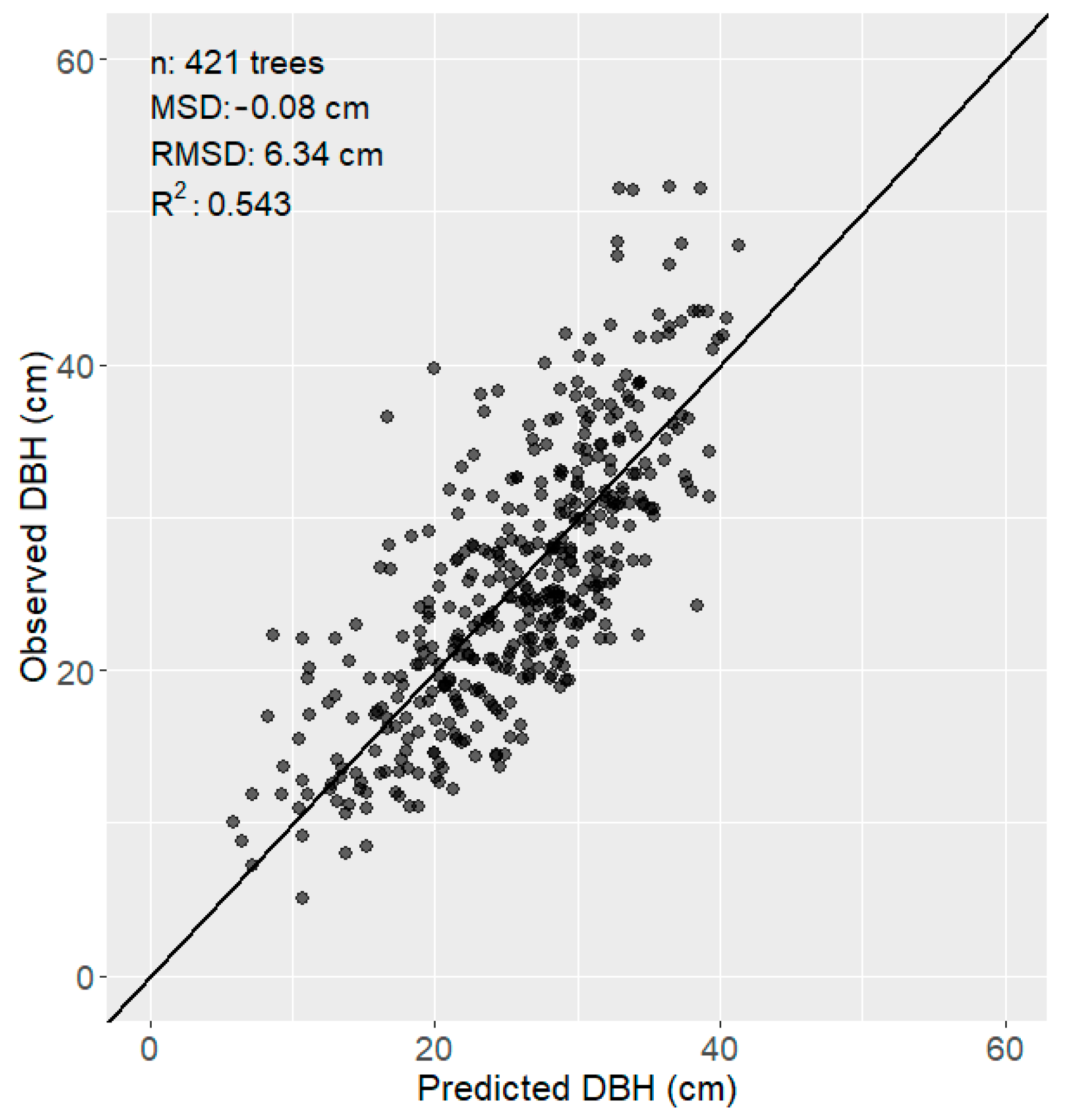
The DBH values of the identified trees were predicted with the diameter-height model (Equation (1)) using the coefficients a = 0.533 and b = 0.054. Figure 3 suggests an overprediction of the model for small DBH and an underprediction for larger DBH with a saturation around 40 cm.
Table 4 presents the number of crowns detected with only one tree, omitted, and detected with more than one tree. The identification of trees based on CHMs with coarser resolution (≥0.75 m) showed a decrease in the number of crowns detected with more than one tree and an increase in the number of dead crowns omitted compared to CHMs with finer resolution. Between 75% and 83% of the dead crowns were detected with only one tree. The tree dataset from CHM_075m was the most performant. It detected 83% of the crowns with only one tree, 3% of the crowns with more than one tree, but omitted 14%. Trees identified in optical data did not perform as well as the tree datasets based on CHMs. Around 60% of the dead crowns were detected with only one tree and almost 25% with more than one tree. However, approximately 15% of the dead crowns were omitted, which was less than the number of dead crowns omitted using CHM_1m.

3.2. Status Identification

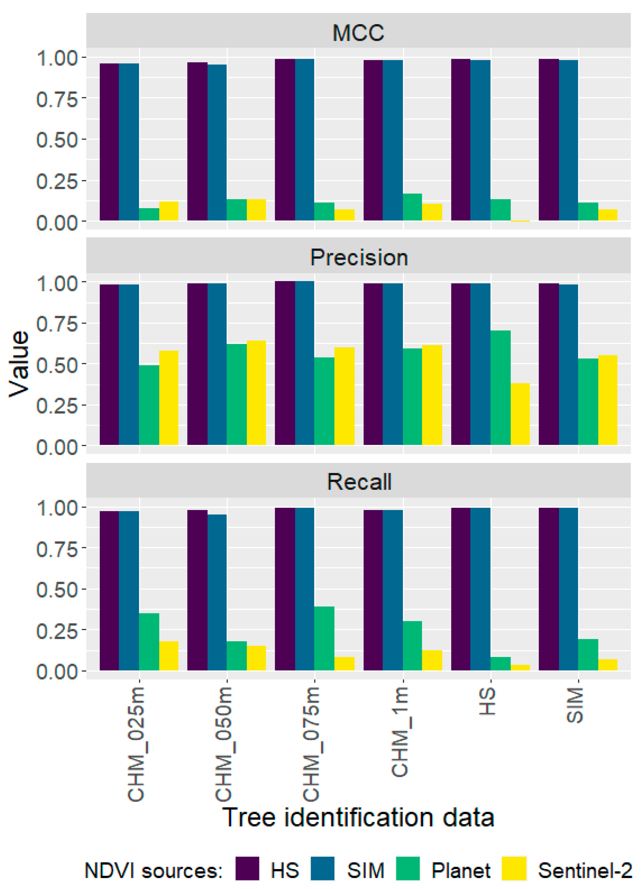
The performance metrics for the predicted status are presented in Figure 4. For the models using NDVI from aerial images (NDVIHS and NDVISIM), MCC values varied from 0.95 to 0.99, suggesting almost perfect predictions. The models using NDVI from satellite images (NDVIPlanet and NDVIS2) showed a low predictive power with values closer to zero. Precision values were larger for both NDVIPlanet and NDVIS2, 0.49 to 0.70 and 0.38 to 0.64, respectively, compared to recall values, 0.08 to 0.39 and 0.02 to 0.18, respectively, suggesting a larger omission rate than commission rate.
Figure 5 illustrates the variation in the predicted status when multiple trees were identified in a crown. The following results do not include the results from the trees identified in CHM_075m and CHM_1m, which had less than 3% of the crowns detected with more than one tree. The predicted status using NDVI from aerial images were mixed in 2% to 8% of the living crowns and 2% to 13% of the dead crowns. However, the percentage of crowns with mixed tree status increased when using NDVI from satellite images, especially for dead crowns. The percentage varied from 4% to 38% and 2% to 14% for living crowns but reached 79% to 95% and 79% to 97% for dead crowns, using NDVIPlanet and NDVIS2, respectively.

3.3. Validation

The predicted density of SDT was validated against the CHI dataset (Table 5). The smallest RMSD and MSD values were obtained for CHMs with coarser spatial resolution (≥0.75 m) and NDVI for aerial images with a RMSD of 34 ha−1 and small negative systematic error of 2 ha−1 when computed from CHM_075m with DBH larger than 20 cm and NDVISIM. Although NDVI from satellite images in combination with CHM_1m resulted in a RMSD close to 60 ha−1, NDVIPlanet presented a small positive systematic error of 3 ha−1 while NDVIS2 had a large negative systematic error of 45 ha−1. In most cases, NDVIS2 led to a statistically significant underestimation of the SDT density and large RMSD values. Trees identified in optical data combined with NDVI from aerial images returned RMSD of SDT near 50 ha−1 and small negative systematic errors close to 15 ha−1. When combined with NDVI from satellite images, trees identified in optical data yielded RMSD values of around 65 ha−1, with negative systematic errors near 20 ha−1 for NDVIPlanet and 50 ha−1 for NDVIS2.
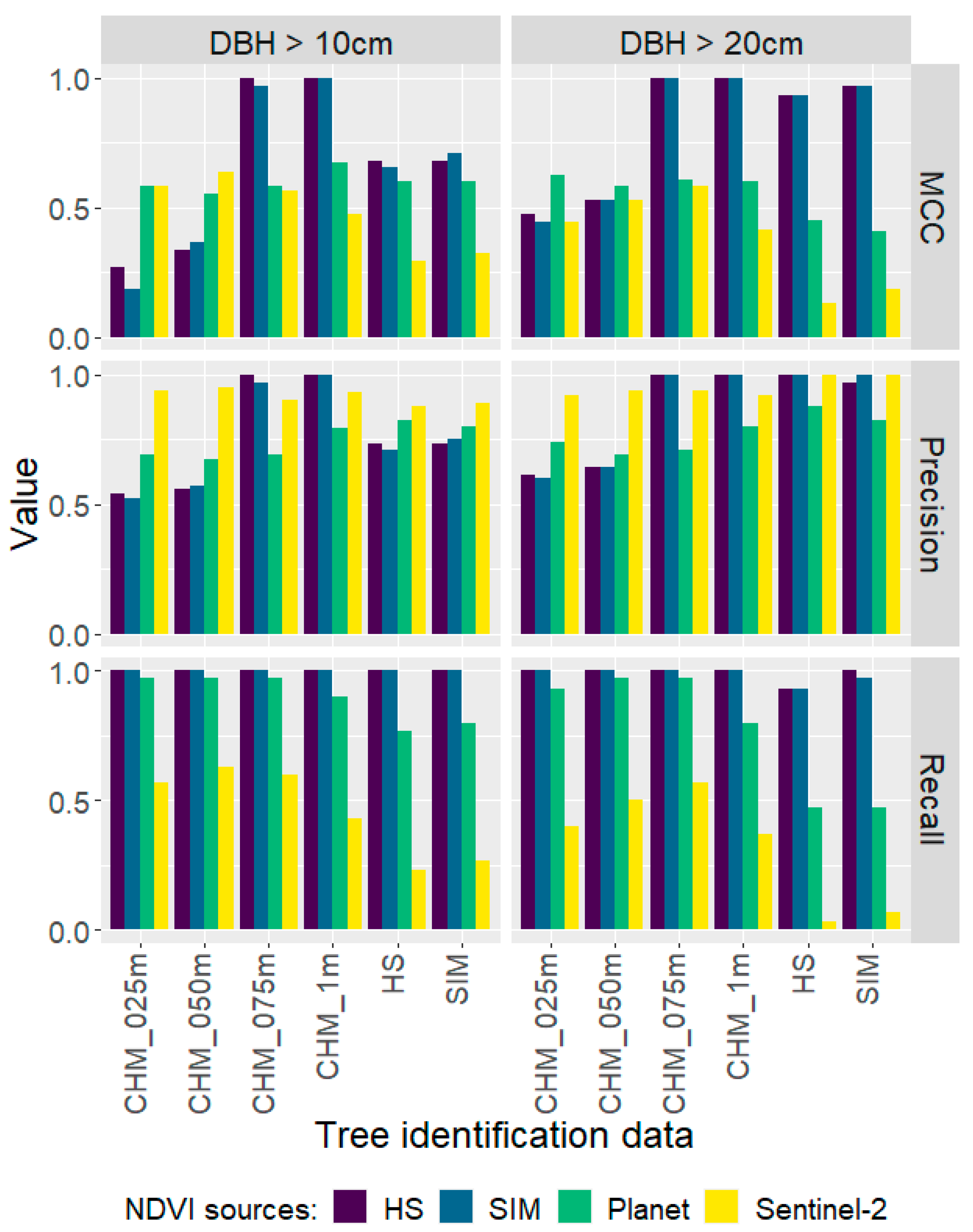
The predicted presence/absence of SDT was validated against the PA dataset (Figure 6). In general, the density of large dead trees (DBH > 20 cm) was found to be a better predictor of presence/absence of SDT when using NDVI from aerial images to determine the status. However, when using NDVI from satellite images, including dead trees of all DBH sizes (DBH > 10 cm), proved to be a better predictor. When combined with NDVI from aerial images, perfect predictions were obtained from trees identified in coarser CHMs datasets (≥0.75 m), and good predictions were achieved from trees identified in optical data, with MCC values ranging from 0.94 to 0.97 for large SDT and from 0.65 to 0.71 for SDT of all DBH sizes, respectively. The presence/absence of SDT was not predicted as accurately with NDVI from satellite images, with MCC values of maximum 0.67. While predictions from NDVIPlanet were similar for all tree datasets, NDVIS2 performed poorly when combined with trees identified in optical data. Figure 7 illustrates the magnitude of the commission errors from the different models by presenting the density of predicted dead trees in both the dead and living PA polygons. Trees identified in CHMs with coarse spatial resolution or in optical data predicted a low density of SDT in the living PA polygons and returned large precision values, implying a small commission error rate. This was also the case for models based on NDVIS2. Recall values were generally large, except with NDVIS2, suggesting a small omission error rate.

4. Discussion

The potential of different RS data sources was assessed to identify trees and to determine their status, i.e., dead or living. By comparing RS data with different spatial and spectral resolutions, we aimed to assess the potential of the proposed tree-based approach to detect SDT for large areas as pre-information to support CHI inventories.
Forests in Norway are spread over 12 degrees in latitude, from 58 N to 70 N, and raise up to almost 1300 m above sea level in south-central Norway [65]. Consequently, variations are observed in tree density, dominant tree species, and tree sizes between geographic zones. To determine objectively the best window size to identify local maxima for a specific area, we proposed to determine whether the number of trees identified was significantly different from the number of trees sampled in the field plots using a paired t-test. While this method yielded good results when performing validation at crown level, it led to poorer results at area level. Small, suppressed trees are hardly detectable from airborne RS data. The number of identified trees was consistent with the number of sample trees due to the balance achieved between omitted suppressed trees and over-sampled dominant trees. It was anticipated that oversampling the dominant trees would enhance the detection rate of snags entangled in living crowns. Although oversampling tree crowns has the potential to negatively impact the results, it was assumed that this impact would be minimized as only trees classified as dead were used to predict the SDT density. However, the approach we chose to predict the status of the trees, based on the status of the crown intersected, led to some misclassification of the tree status, and therefore a smaller accuracy at area level. As a result, trees identified in CHMs with coarser spatial resolutions were performing better than trees identified in CHMs with finer resolutions. Although trees identified in CHMs with coarser resolution omitted up to 25% of the dead crowns, they targeted more dominant trees, did not oversampled crowns, and detected most of the large snags. The window size used to identify local maxima had presumably more impact on the accuracy of the tree identification than the resolution of the image itself. Therefore, better results could be achieved using finer CHM resolutions with larger window sizes to find local maxima, considering the filter size limitation to odd multiples of the raster resolution.
The risk of confusion between ground vegetation and forest cover poses a challenge to identify trees using optical images. We extracted the height of the trees from a CHM_025m, and used their predicted DBH to exclude trees with DBH smaller than 10 cm. As an alternative to CHMs, ground vegetation and forest cover could be discriminated using a supervised classification method [48,66] or a histogram-based thresholding method [67].
The distribution of the NDVI values diverged between the different sensors/datasets and therefore no common threshold could be used to discriminate between dead and living trees. A preliminary assessment suggested that, while a threshold around 0.5 would perform well on NDVIHS and NDVISIM, a larger threshold would be required for NDVIPlanet and smaller for NDVIS2. A possible explanation is that PlanetScope data cover a larger range of wavelengths in the red part of the spectrum, while Sentinel-2 covers a larger range in the NIR part. Instead, we built models based on the status observed in the crown dataset to predict the status of the identified trees. The crowns were visually delineated using HS data and a CHM. Only crowns that were clearly dead, or clearly living were selected. Although living crowns with dead apex or branches were a common phenomenon in the study area, they were excluded from the crown dataset. Since we extracted the NDVI values at the local maxima location, i.e., for one pixel only, this approach may have led to the misclassification of healthy trees as dead if there were dead branches near the apex. In addition, ref. [68] reported a negative effect of the slope on the tree detection, leading to horizontal and/or vertical displacements of the tree apex of more than a meter in extreme cases, and therefore extraction of the wrong pixel to determine the status. An alternative to the extraction of a single pixel could be to average the pixel values within a buffer distance from the location of the local maximum. This, however, would considerably increase the processing time. Another option could be to apply a smoothing filter on the image before identifying local maxima. It was reported by [57] that filtering the images reduced the detected number of local maxima, and depending on the filter size and the conditions of the applied filter, lead to an increased accuracy of the predictions for stem number.
Although the tree status was perfectly predicted using NDVI from aerial images in combination with any tree dataset, MCC values close to zero were obtained when using NDVI from satellite images. This low predictive power was mainly caused by omission errors, especially with NDVIS2. The average crown sizes were 8.0 m2 for living crowns and 3.4 m2 for dead crowns. Pixel values from PlanetScope and Sentinel-2 images are consequently a mix of adjacent tree crowns and background values. There is therefore a larger probability of detecting living crowns than dead crowns due to their respective average crown sizes. For NDVI from satellite images, it might be more appropriate to use trees with DBH larger than 20 cm to build the predictive models for determination of tree status. Another alternative could be to define a fixed threshold for classifying dead and living trees using reference areas of sizes suitable for the resolution of the NDVI source.
There was no clear difference in the results between NDVIHS and NDVISIM. NDVIHS was expected to yield better results considering the narrow spectral wavelength chosen to produce the index, but only a few examples were found where NDVIHS performed better than NDVISIM. Most of them were cases of suppressed living trees found in the shadow, correctly classified by NDVIHS but identified as dead by NDVISIM.
The tree-based approach performed better for predicting presence/absence of SDT than the density. This difference in performance can be partly explained by the validation dataset used to evaluate the predictions. While the accuracy of the predicted density of SDT was assessed with the CHI dataset, the presence/absence was validated against the PA dataset. The small overlap reached by the two sets of SDT polygons provided by companies A and B, combined in this study to create the CHI dataset, illustrates the challenge of identifying SDT in the field. The polygons in the CHI dataset were delineated in the field, assessing the tree status from under the canopy, while the polygons in the PA dataset were delineated from the HS image, assessing the tree status from above the canopy. The PA dataset is therefore likely to be more closely associated with predictions obtained from RS data. In addition, the polygons in the CHI dataset were clipped to fit the extent of the old and mature forest stands. Areas with large density of SDT might have been excluded, changing the density of SDT in the polygons.
NDVI is a widely recognized vegetation index that provides the ability to differentiate between healthy and dead vegetation and can be computed from any optical images containing red and NIR bands. Furthermore, the use of ALS data has gained popularity worldwide as a tool for assessing various forest attributes. Many countries have now acquired a full coverage of ALS data for their forests, and in many cases have made the data publicly available. Combining ALS data with NDVI data provides valuable insight into forest structure and dynamics, making it useful for forest management and conservation on a global scale. Furthermore, the use of satellite-derived NDVI enables large-scale comparisons between different countries and regions.

5. Conclusions

Knowledge about the exact location and extent of areas rich in deadwood are important from a management perspective, particularly with regard to preserving biodiversity. In light of our results, we conclude that it would be possible to use a tree-based approach to detect the presence of SDT for large areas using CHMs with spatial resolutions of 1 m or finer and optical images of medium spatial resolution, i.e., 3 m or finer, including a NIR band. After comparing different RS data sources, we concluded that, while optical images could be used to identify trees, CHMs derived from ALS data provided a more performant solution. Although the identification of the tree status was better achieved with optical images of finer spatial resolution, finer spectral resolution did not seem to improve the results. The use of RS data following a tree-based approach can provide a more objective and systematic approach for producing maps of presence/absence of deadwood for larger areas as pre-information to support forest management planning at municipality level or to update existing CHI information.

Author Contributions

Conceptualization, M.-C.J.-P., T.G., E.N. and H.O.Ø.; methodology, M.-C.J.-P. and H.O.Ø.; formal analysis, M.-C.J.-P. and H.O.Ø.; writing—original draft preparation, M.-C.J.-P.; writing—review and editing, M.-C.J.-P., T.G., E.N. and H.O.Ø.; visualization, M.-C.J.-P.; project administration, T.G. and H.O.Ø.; funding acquisition, T.G., E.N. and H.O.Ø. All authors have read and agreed to the published version of the manuscript.

Funding

This study was funded by PreMiNa, “Evaluation of remote sensing data as pre-information for woodland key habitat mapping according to the EcoSyst framework” and the project NOBEL, “Novel business models and mechanisms for the sustainable supply of and payment for forest ecosystem services”. The PreMiNa project is funded by the private research fund, Skogtiltaksfondet, the Forest Trust Fund (Utviklingsfondet for skogbruket), and private forest owners’ associations in Norway. The project NOBEL is supported under the umbrella of ERA-NET Cofund ForestValue. ForestValue has received funding from the European Union’s Horizon 2020 research and innovation program under grant agreement N° 773324. Furthermore, the study was supported by the Norwegian Research Council (project number 297883).

Data Availability Statement

The data presented in this study are available on request from the corresponding author. Restrictions apply to the availability of the CHI dataset. Data were obtained from the Norwegian Agricultural Agency and are available from the authors with the permission of the Norwegian Agricultural Agency.

Acknowledgments

The authors would like to thank Terratec AS, Norway, for collecting and processing the ALS and HS data. We would also like to thank the Norwegian Agriculture Agency for organizing and sharing the CHI field survey and Glommen Mjøsen Skog SA for conducting the sample plot inventory. Finally, we would like to acknowledge Michele Dalponte of the Department of Sustainable Agro-Ecosystems and Bioresources, Research and Innovation Center Fondazione Edmund Mach, San Michele all’ Adige, Italy for processing and mosaicking the hyperspectral images.

Conflicts of Interest

The authors declare no conflict of interest. The funders had no role in the design of the study; in the collection, analyses, or interpretation of data; in the writing of the manuscript; or in the decision to publish the results.

References

  1. Costanza, R.; de Groot, R.; Braat, L.; Kubiszewski, I.; Fioramonti, L.; Sutton, P.; Farber, S.; Grasso, M. Twenty years of ecosystem services: How far have we come and how far do we still need to go? Ecosyst. Serv. 2017, 28, 1–16. [Google Scholar] [CrossRef]
  2. IPBES. Summary for Policymakers of the Global Assessment Report on Biodiversity and Ecosystem Services of the Intergovernmental Science-Policy Platform on Biodiversity and Ecosystem Services; Díaz, S., Settele, J., Brondizio, E.S., Eds.; IPBES Secretariat: Bonn, Germany, 2019; p. 56. [Google Scholar] [CrossRef]
  3. Lonsdale, D.; Pautasso, M.; Holdenrieder, O. Wood-decaying fungi in the forest: Conservation needs and management options. Eur. J. For. Res. 2008, 127, 1–22. [Google Scholar] [CrossRef]
  4. Siitonen, J. Forest Management, Coarse Woody Debris and Saproxylic Organisms: Fennoscandian Boreal Forests as an Example. Ecol. Bull. 2001, 49, 11–41. [Google Scholar]
  5. Bradshaw, C.J.A.; Warkentin, I.G.; Sodhi, N.S. Urgent preservation of boreal carbon stocks and biodiversity. Trends Ecol. Evol. 2009, 24, 541–548. [Google Scholar] [CrossRef]
  6. Stokland, J.N.; Tomter, S.M.; Söderberg, U. Development of dead wood indicators for biodiversity monitoring: Experiences from Scandinavia. Monit. Indic. For. Biodivers. Eur.—Ideas Oper. 2004, 51, 207–226. [Google Scholar]
  7. Harmon, M.E.; Franklin, J.F.; Swanson, F.J.; Sollins, P.; Gregory, S.V.; Lattin, J.D.; Anderson, N.H.; Cline, S.P.; Aumen, N.G.; Sedell, J.R.; et al. Ecology of Coarse Woody Debris in Temperate Ecosystems. Adv. Ecol. Res. 1986, 15, 133–302. [Google Scholar]
  8. Stokland, J.N.; Siitonen, J.; Jonsson, B.G. Biodiversity in Dead Wood; Cambridge University Press: Cambridge, UK, 2012. [Google Scholar]
  9. Esseen, P.-A.; Ehnström, B.; Ericson, L.; Sjöberg, K. Boreal Forests. Ecol. Bull. 1997, 46, 16–47. [Google Scholar]
  10. Franklin, J.F.; Shugart, H.H.; Harmon, M.E. Tree Death as an Ecological Process. BioScience 1987, 37, 550–556. [Google Scholar] [CrossRef]
  11. Hansen, A.J.; Spies, T.A.; Swanson, F.J.; Ohmann, J.L. Conserving Biodiversity in Managed Forests. BioScience 1991, 41, 382–392. [Google Scholar] [CrossRef]
  12. Kuuluvainen, T. Natural variability of forests as a reference for restoring and managing biological diversity in boreal Fennoscandia. Silva Fenn. 2002, 36, 97–125. [Google Scholar] [CrossRef]
  13. Gjerde, I.; Sætersdal, M.; Blom, H.H. Complementary Hotspot Inventory—A method for identification of important areas for biodiversity at the forest stand level. Biol. Conserv. 2007, 137, 549–557. [Google Scholar] [CrossRef]
  14. Timonen, J.; Siitonen, J.; Gustafsson, L.; Kotiaho, J.S.; Stokland, J.N.; Sverdrup-Thygeson, A.; Mönkkönen, M. Woodland key habitats in northern Europe: Concepts, inventory and protection. Scand. J. For. Res. 2010, 25, 309–324. [Google Scholar] [CrossRef]
  15. Lindenmayer, D.B.; Franklin, J.F. Conserving Forest Biodiversity: A Comprehensive Multiscaled Approach; Island Press: Washington, DC, USA, 2002. [Google Scholar]
  16. Gjerde, I.; Sætersdal, M.; Rolstad, J.; Blom, H.H.; Storaunet, K.O. Fine-scale diversity and rarity hotspots in northern forests. Conserv. Biol. 2004, 18, 1032–1042. [Google Scholar] [CrossRef]
  17. Hansson, L. Key Habitats in Swedish Managed Forests. Scand. J. For. Res. 2001, 16, 52–61. [Google Scholar] [CrossRef]
  18. Baumann, C.; Gjerde, I.; Blom, H.H.; Sætersdal, M.; Nilsen, J.-E.; Løken, B.; Ekanger, I. Environmental Inventories in Forests—Biodiversity. Part 1: Background and Principles; Skogforsk and Norwegian Ministry of Agriculture: Uppsala, Sweden, 2002. [Google Scholar]
  19. PEFC Norway. Norwegian PEFC Forest Standard; PEFC Norway: Oslo, Norway, 2015; p. 31. [Google Scholar]
  20. Baumann, C.; Gjerde, I.; Blom, H.H.; Sætersdal, M.; Nilsen, J.-E.; Løken, B.; Ekanger, I. Environmental Inventories in Forests—Biodiversity. Part 2: Forest Habitats; Skogforsk and the Norwegian Ministry of Agriculture: Uppsala, Sweden, 2002. [Google Scholar]
  21. Haga, H.E.; Nilsen, A.B.; Ullerud, H.A.; Bryn, A. Quantification of accuracy in field-based land cover maps: A new method to separate different components. Appl. Veg. Sci. 2021, 24, e12578. [Google Scholar] [CrossRef]
  22. Eriksen, E.L.; Ullerud, H.A.; Halvorsen, R.; Aune, S.; Bratli, H.; Horvath, P.; Volden, I.K.; Wollan, A.K.; Bryn, A. Point of view: Error estimation in field assignment of land-cover types. Phytocoenologia 2018, 49, 135–148. [Google Scholar] [CrossRef]
  23. Ørka, H.O.; Jutras-Perreault, M.-C.; Candelas-Bielza, J.; Gobakken, T. Delineation of Geomorphological Woodland Key Habitats Using Airborne Laser Scanning. Remote Sens. 2022, 14, 1184. [Google Scholar] [CrossRef]
  24. Magnussen, S.; Boudewyn, P. Derivations of stand heights from airborne laser scanner data with canopy-based quantile estimators. Can. J. For. Res. 1998, 28, 1016–1031. [Google Scholar] [CrossRef]
  25. Maltamo, M.; Packalen, P. Species-specific management inventory in Finland. In Forestry Applications of Airborne Laser Scanning; Springer: Dordrecht, The Netherlands, 2014; pp. 241–252. [Google Scholar]
  26. Næsset, E. Accuracy of forest inventory using airborne laser scanning: Evaluating the first nordic full-scale operational project. Scand. J. For. Res. 2004, 19, 554–557. [Google Scholar] [CrossRef]
  27. Næsset, E. Practical large-scale forest stand inventory using a small-footprint airborne scanning laser. Scand. J. For. Res. 2004, 19, 164–179. [Google Scholar] [CrossRef]
  28. Næsset, E. Area-based inventory in Norway—From innovation to an operational reality. In Forestry Applications of Airborne Laser Scanning; Springer: Dordrecht, The Netherlands, 2014; pp. 215–240. [Google Scholar]
  29. Kim, Y.; Yang, Z.; Cohen, W.B.; Pflugmacher, D.; Lauver, C.L.; Vankat, J.L. Distinguishing between live and dead standing tree biomass on the North Rim of Grand Canyon National Park, USA using small-footprint lidar data. Remote Sens. Environ. 2009, 113, 2499–2510. [Google Scholar] [CrossRef]
  30. Martinuzzi, S.; Vierling, L.A.; Gould, W.A.; Falkowski, M.J.; Evans, J.S.; Hudak, A.T.; Vierling, K.T. Mapping snags and understory shrubs for a LiDAR-based assessment of wildlife habitat suitability. Remote Sens. Environ. 2009, 113, 2533–2546. [Google Scholar] [CrossRef]
  31. Pesonen, A.; Maltamo, M.; Eerikäinen, K.; Packalèn, P. Airborne laser scanning-based prediction of coarse woody debris volumes in a conservation area. For. Ecol. Manag. 2008, 255, 3288–3296. [Google Scholar] [CrossRef]
  32. Bekkar, M.; Djemaa, H.K.; Alitouche, T.A. Evaluation measures for models assessment over imbalanced data sets. J. Inf. Eng. Appl. 2013, 3, 27–38. [Google Scholar]
  33. Chicco, D.; Jurman, G. The advantages of the Matthews correlation coefficient (MCC) over F1 score and accuracy in binary classification evaluation. BMC Genom. 2020, 21, 6. [Google Scholar] [CrossRef]
  34. Jutras-Perreault, M.-C.; Næsset, E.; Gobakken, T.; Ørka, H.O. Detecting the presence of standing dead trees using airborne laser scanning and optical data. under revision.
  35. Li, W.; Guo, Q.; Jakubowski, M.K.; Kelly, M. A new method for segmenting individual trees from the lidar point cloud. Photogramm. Eng. Remote Sens. 2012, 78, 75–84. [Google Scholar] [CrossRef]
  36. Rahman, M.Z.A.; Gorte, B.; Bucksch, A.K. A new method for individual tree measurement from airborne LiDAR. In Proceedings of the Silvilaser, College Station, TX, USA, 14–16 October 2009; pp. 14–16. [Google Scholar]
  37. Solberg, S.; Naesset, E.; Bollandsas, O.M. Single tree segmentation using airborne laser scanner data in a structurally heterogeneous spruce forest. Photogramm. Eng. Remote Sens. 2006, 72, 1369–1378. [Google Scholar] [CrossRef]
  38. Popescu, S.C.; Wynne, R.H. Seeing the Trees in the Forest: Using Lidar and Multispectral Data Fusion with Local Filtering and Variable Window Size for Estimating Tree Height. Photogramm. Eng. Remote Sens. 2004, 70, 589–604. [Google Scholar] [CrossRef]
  39. Ene, L.; Næsset, E.; Gobakken, T. Single tree detection in heterogeneous boreal forests using airborne laser scanning and area-based stem number estimates. Int. J. Remote Sens. 2012, 33, 5171–5193. [Google Scholar] [CrossRef]
  40. Wang, L.; Gong, P.; Biging, G.S. Individual tree-crown delineation and treetop detection in high-spatial-resolution aerial imagery. Photogramm. Eng. Remote Sens. 2004, 70, 351–357. [Google Scholar] [CrossRef]
  41. Korpela, I.; Anttila, P.; Pitkänen, J. The performance of a local maxima method for detecting individual tree tops in aerial photographs. Int. J. Remote Sens. 2006, 27, 1159–1175. [Google Scholar] [CrossRef]
  42. Wulder, M.; Niemann, K.O.; Goodenough, D.G. Local maximum filtering for the extraction of tree locations and basal area from high spatial resolution imagery. Remote Sens. Environ. 2000, 73, 103–114. [Google Scholar] [CrossRef]
  43. Lefsky, M.A.; Cohen, W.B.; Acker, S.A.; Parker, G.G.; Spies, T.A.; Harding, D. Lidar Remote Sensing of the Canopy Structure and Biophysical Properties of Douglas-Fir Western Hemlock Forests. Remote Sens. Environ. 1999, 70, 339–361. [Google Scholar] [CrossRef]
  44. Wing, B.M.; Ritchie, M.W.; Boston, K.; Cohen, W.B.; Olsen, M.J. Individual snag detection using neighborhood attribute filtered airborne lidar data. Remote Sens. Environ. 2015, 163, 165–179. [Google Scholar] [CrossRef]
  45. Bütler, R.; Schlaepfer, R. Spruce snag quantification by coupling colour infrared aerial photos and a GIS. For. Ecol. Manag. 2004, 195, 325–339. [Google Scholar] [CrossRef]
  46. Pasher, J.; King, D.J. Mapping dead wood distribution in a temperate hardwood forest using high resolution airborne imagery. For. Ecol. Manag. 2009, 258, 1536–1548. [Google Scholar] [CrossRef]
  47. Haara, A.; Nevalainen, S. Detection of dead or defoliated spruces using digital aerial data. For. Ecol. Manag. 2002, 160, 97–107. [Google Scholar] [CrossRef]
  48. Fassnacht, F.E.; Latifi, H.; Ghosh, A.; Joshi, P.K.; Koch, B. Assessing the potential of hyperspectral imagery to map bark beetle-induced tree mortality. Remote Sens. Environ. 2014, 140, 533–548. [Google Scholar] [CrossRef]
  49. Lausch, A.; Heurich, M.; Gordalla, D.; Dobner, H.-J.; Gwillym-Margianto, S.; Salbach, C. Forecasting potential bark beetle outbreaks based on spruce forest vitality using hyperspectral remote-sensing techniques at different scales. For. Ecol. Manag. 2013, 308, 76–89. [Google Scholar] [CrossRef]
  50. Zielewska-Büttner, K.; Adler, P.; Kolbe, S.; Beck, R.; Ganter, L.M.; Koch, B.; Braunisch, V. Detection of Standing Deadwood from Aerial Imagery Products: Two Methods for Addressing the Bare Ground Misclassification Issue. Forests 2020, 11, 801. [Google Scholar] [CrossRef]
  51. Maltamo, M.; Kallio, E.; Bollandsås, O.M.; Næsset, E.; Gobakken, T.; Pesonen, A. Assessing Dead Wood by Airborne Laser Scanning. In Forestry Applications of Airborne Laser Scanning; Springer: Dordrecht, The Netherlands, 2014; pp. 375–395. [Google Scholar]
  52. Landbruksdirektoratet. Veileder for Kartlegging av MiS-Livsmiljøer Etter NiN (Guide for Mapping MiS Habitats According to NiN); Landbruksdirektoratet: Oslo, Norway, 2017; p. 26. [Google Scholar]
  53. Cover, T.; Hart, P. Nearest neighbor pattern classification. IEEE Trans. Inf. Theory 1967, 13, 21–27. [Google Scholar] [CrossRef]
  54. Shepard, D. A two-dimensional interpolation function for irregularly-spaced data. In Proceedings of the 1968 23rd ACM National Conference, New York, NY, USA, 27–29 August 1968; pp. 517–524. [Google Scholar] [CrossRef]
  55. Baldi, P.; Brunak, S.; Chauvin, Y.; Andersen, C.A.; Nielsen, H. Assessing the accuracy of prediction algorithms for classification: An overview. Bioinformatics 2000, 16, 412–424. [Google Scholar] [CrossRef] [PubMed]
  56. Chai, T.; Draxler, R.R. Root mean square error (RMSE) or mean absolute error (MAE)?–Arguments against avoiding RMSE in the literature. Geosci. Model Dev. 2014, 7, 1247–1250. [Google Scholar] [CrossRef]
  57. Lindberg, E.; Hollaus, M. Comparison of methods for estimation of stem volume, stem number and basal area from airborne laser scanning data in a hemi-boreal forest. Remote Sens. 2012, 4, 1004–1023. [Google Scholar] [CrossRef]
  58. Heinzel, J.N.; Weinacker, H.; Koch, B. Prior-knowledge-based single-tree extraction. Int. J. Remote Sens. 2011, 32, 4999–5020. [Google Scholar] [CrossRef]
  59. Dalponte, M.; Ørka, H.O.; Ene, L.T.; Gobakken, T.; Næsset, E. Tree crown delineation and tree species classification in boreal forests using hyperspectral and ALS data. Remote Sens. Environ. 2014, 140, 306–317. [Google Scholar] [CrossRef]
  60. Dalponte, M.; Reyes, F.; Kandare, K.; Gianelle, D. Delineation of individual tree crowns from ALS and hyperspectral data: A comparison among four methods. Eur. J. Remote Sens. 2015, 48, 365–382. [Google Scholar] [CrossRef]
  61. Clark, M.L.; Roberts, D.A.; Clark, D.B. Hyperspectral discrimination of tropical rain forest tree species at leaf to crown scales. Remote Sens. Environ. 2005, 96, 375–398. [Google Scholar] [CrossRef]
  62. Bi, H.; Fox, J.C.; Li, Y.; Lei, Y.; Pang, Y. Evaluation of nonlinear equations for predicting diameter from tree height. Can. J. For. Res. 2012, 42, 789–806. [Google Scholar] [CrossRef]
  63. Ryu, J.-H.; Na, S.-I.; Cho, J. Inter-Comparison of normalized difference vegetation index measured from different footprint sizes in cropland. Remote Sens. 2020, 12, 2980. [Google Scholar] [CrossRef]
  64. Van Leeuwen, W.J.; Orr, B.J.; Marsh, S.E.; Herrmann, S.M. Multi-sensor NDVI data continuity: Uncertainties and implications for vegetation monitoring applications. Remote Sens. Environ. 2006, 100, 67–81. [Google Scholar] [CrossRef]
  65. Norwegian Mapping Authority. The N50 Topographic Map Series of Norway. Scale 1:50,000; Updated in 2007; Norwegian Mapping Authority: Hønefoss, Norway, 2017. [Google Scholar]
  66. Huang, C.; Davis, L.; Townshend, J. An assessment of support vector machines for land cover classification. Int. J. Remote Sens. 2002, 23, 725–749. [Google Scholar] [CrossRef]
  67. Otsu, N. A threshold selection method from gray-level histograms. IEEE Trans. Syst. Man Cybern. 1979, 9, 62–66. [Google Scholar] [CrossRef]
  68. Khosravipour, A.; Skidmore, A.K.; Wang, T.; Isenburg, M.; Khoshelham, K. Effect of slope on treetop detection using a LiDAR Canopy Height Model. ISPRS J. Photogramm. Remote Sens. 2015, 104, 44–52. [Google Scholar] [CrossRef]
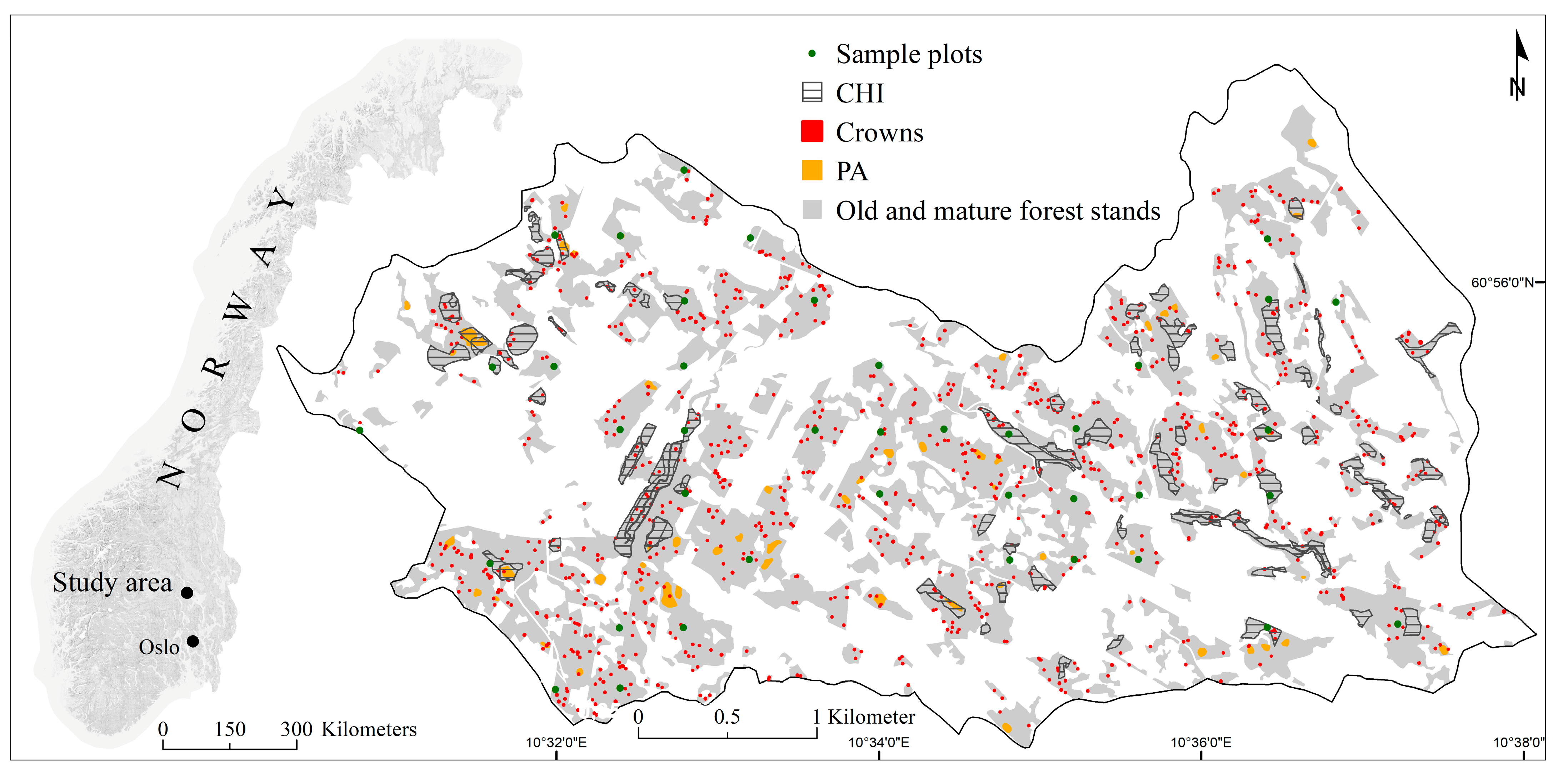
Figure 1. Study area location in south-eastern Norway. Distribution of sample plots, Complementarity Hotspot Inventory (CHI), presence/absence (PA) and tree crown polygons within old and mature forests. The PA dataset contains polygons delineating forested areas dominated by standing dead trees (presence) and dominated by living trees (absence). Sample plots and tree crown extents were enlarged to be visible on the map.
Remotesensing 15 02223 g001
Figure 2. Flow chart describing the procedure followed for predicting the density and the presence/absence of standing dead trees (SDT). The trees were identified using canopy height models (CHM) of 0.25 m, 0.50 m, 0.75 m, and 1 m spatial resolution (CHM_025m, CHM_050m, CHM_075m and CHM_1m) and on hyperspectral (HS) and simulated aerial image (SIM). The density and presence/absence of SDT were validated using the Complementary Hotspot Inventory (CHI) dataset and the presence/absence (PA) dataset, respectively. DBH: diameter at breast height. Grey boxes: main steps; dashed lines: validation steps; dashed-dotted lines: validation step used to define parameters.
Remotesensing 15 02223 g002
Figure 3. Scatter plot of observed and predicted diameter at breast height (DBH). n: number of sample trees; MSD: mean signed difference; RMSD: root-mean-square difference.
Remotesensing 15 02223 g003
Figure 4. Agreement between observed status of the crowns and predicted status of the trees. The trees were identified using canopy height models (CHM) of 0.25 m, 0.50 m, 0.75 m, and 1 m spatial resolution (CHM_025m, CHM_050m, CHM_075m and CHM_1m) and in hyperspectral (HS) and simulated aerial image (SIM).
Remotesensing 15 02223 g004
Figure 5. Status of trees located withing crowns detected with more than one tree. Living: living crown with only living trees; living mixed: living crowns with both dead and living trees; dead: dead crowns with only dead trees; dead mixed: dead crowns with both dead and living trees. The trees were identified using canopy height models (CHM) of 0.25 m, 0.50 m, 0.75 m, and 1 m spatial resolution (CHM_025m, CHM_050m, CHM_075m, and CHM_1m) and in hyperspectral (HS) and simulated aerial image (SIM).
Remotesensing 15 02223 g005
Figure 6. Agreement between the predicted presence/absence of standing dead trees (SDT) and the presence/absence (PA) dataset for SDT with diameter at breast height (DBH) larger than 10 cm and larger than 20 cm. The trees were identified using canopy height models (CHM) of 0.25 m, 0.50 m, 0.75 m, and 1 m spatial resolution (CHM_025m, CHM_050m, CHM_075m, and CHM_1m) and in hyperspectral (HS) and simulated aerial image (SIM).
Remotesensing 15 02223 g006
Figure 7. Predicted density of standing dead trees (SDT) in presence/absence (PA) polygons dominated by dead trees (dead) and living trees (living) for SDT with diameter at breast height (DBH) larger than 10 cm and larger than 20 cm. The trees were identified using canopy height models (CHM) of 0.25 m, 0.50 m, 0.75 m, and 1 m spatial resolution (CHM_025m, CHM_050m, CHM_075m, and CHM_1m) and in hyperspectral (HS) and simulated aerial image (SIM). The tree status was predicted using NDVI from HS, SIM, PlanetScope (Planet), and Sentinel-2 images.
Remotesensing 15 02223 g007
Table 1. Characteristics of the crown, Complementary Hotspot Inventory (CHI) and presence/absence (PA) datasets regarding their polygon numbers (n) and sizes. SD: Standard deviation.
nRange (m2)Mean (m2)SD
Crowns
Living500[0.8–66.4]8.05.3
Dead500[0.3–18.6]3.42.7
CHI
Density of SDT43[750–36380]88937904
PA *
Living30[304–2187]1022454
Dead30[43–6645]14241534
* Areas dominated by living or dead trees.
Table 2. Spatial and spectral resolutions of red and near-infrared (NIR) bands for hyperspectral image (HS), simulated aerial image (SIM), PlanetScope (Planet), and Sentinel-2 images.
Optical DataSpatial Resolution (m)Spectral Resolution Red Band (nm)Spectral Resolution NIR Band (nm)
HS0.3660–667830–836
Sim0.3600–680680–850
Planet3590–670780–860
Sentinel-210650–680785–899
Table 3. Results of paired t-tests and descriptive statistics for the number of observed and identified trees using different window sizes (ws) to find local maxima. The trees were identified in canopy height models (CHM) of 0.25 m, 0.50 m, 0.75 m, and 1 m spatial resolution (CHM_025m, CHM_050m, CHM_075m, and CHM_1m) and in simulated aerial image (SIM). In bold: mean difference not statistically significantly different from zero. n = number of sample trees/identified trees, M = mean, SD = standard deviation, MSD = mean signed difference, SE = standard error, t = t-test, p = p-value.
Reference
wsnMSDMSDSEtp
Reference 1016259.5
CHM_025m51355349.48.51.74.9<0.001
7641164.5−9.41.1−8.7<0.001
9492123.4−13.11.1−12.2<0.001
CHM_050m31055267.21.01.50.60.529
5455113.1−14.01.2−12.1<0.001
CHM_075m3508133.1−12.71.1−11.5<0.001
CHM_1m3381102.2−15.91.3−12.3<0.001
SIM51194307.54.51.43.20.003
7706184.0−7.81.2−6.3<0.001
9539133.7−11.91.2−9.7<0.001
Table 4. Relation between crowns and number of identified trees. Number of living and dead crowns omitted, detected with only one tree (Detected), and detected with more than one tree (Detected > 1 tree). The trees were identified using canopy height models (CHM) of 0.25 m, 0.50 m, 0.75 m, and 1 m spatial resolution (CHM_025m, CHM_050m, CHM_075m, and CHM_1m) and in hyperspectral (HS) and simulated aerial image (SIM). In parenthesis are the proportion of crowns for every category.
Living CrownsDead Crowns
OmittedDetectedDetected > 1 TreeOmittedDetectedDetected > 1 Tree
CHM_025m13511481738994
(0.00)(0.70)(0.30)(0.03)(0.78)(0.19)
CHM_050m23931053040268
(0.00)(0.79)(0.21)(0.06)(0.80)(0.14)
CHM_075m8477157041614
(0.02)(0.95)(0.03)(0.14)(0.83)(0.03)
CHM_1m2247441233743
(0.04)(0.95)(0.01)(0.25)(0.75)(0.01)
HS1327121678303119
(0.03)(0.54)(0.43)(0.16)(0.61)(0.24)
SIM1226622273310117
(0.02)(0.53)(0.44)(0.15)(0.62)(0.23)
Table 5. Comparison between the density of standing dead trees (SDT) reported in the Complementary Hotspot Inventory (CHI) dataset (mean: 56 ha−1, standard deviation: 24 ha−1) and the predicted densities of SDT with diameter at breast height (DBH) larger than 10 cm and larger than 20 cm. The trees were identified using canopy height models (CHM) of 0.25 m, 0.50 m, 0.75 m, and 1 m spatial resolution (CHM_025m, CHM_050m, CHM_075m, and CHM_1m) and in hyperspectral (HS) and simulated aerial image (SIM). RMSD: root-mean-square difference; MSD: mean signed difference; n ha−1: density of trees per hectare; % mean: percentage of the mean.
DBH > 10 cmDBH > 20 cm
RMSDMSDRMSDMSD
Tree DatasetsNDVIn ha−1% meann ha−1% meann ha−1% meann ha−1% mean
CHM_025mHS289520231416169304111200
SIM305548250449181326124224
Planet332597221397249449144259
S2101181−1−270126−33−59
CHM_050mHS19635215327611520873131
SIM18533214125310819564115
Planet275495183329223402132237
S2911630169124−23−41
CHM_075mHS488717313563−4−8
SIM498920373462−2−4
Planet1262277613710719256102
S262112−16−295599−29−51
CHM_1mHS3666−14−263665−23−41
SIM3665−14−253665−23−41
Planet611097135810435
S256100−41−7456101−45−81
HSHS113203681224988−7−13
SIM116208721304989−6−11
Planet127229356365117−22−39
S289160−35−6364116−48−86
SIMHS104187641154785−9−16
SIM107192681224785−8−15
Planet137247417469124−20−35
S287157−32−5864116−47−85
Disclaimer/Publisher’s Note: The statements, opinions and data contained in all publications are solely those of the individual author(s) and contributor(s) and not of MDPI and/or the editor(s). MDPI and/or the editor(s) disclaim responsibility for any injury to people or property resulting from any ideas, methods, instructions or products referred to in the content.