Abstract
Long-range surveillance and early warning of space targets are significant factors in space security. Under remote observation conditions, the energy performance of the target is weak and subject to environmental and imaging process contamination. Most detection methods are aimed at targets with a high signal-to-noise ratio (SNR) or local contrast, and the detection performance for dim-weak small targets is poor; therefore, the target signal is often enhanced by energy accumulation. However, owing to the interference caused by the instability of the imaging system, energy accumulation errors occur in the target, resulting in the dispersion of the target energy, making detection a challenge. To solve the above problem, this study proposed a multi-frame superposition detection method for dim-weak point targets based on an optimized clustering algorithm by combining the clustering method with the inherent features of the target and using the difference between the target and noise energy distribution for detection. First, we simulated the multi-frame imaging process of the target post-disturbance and established an optical imaging system model of the dim-weak target. Subsequently, we used data dimension reduction and outlier removal to extract the target potential area. Finally, the data were sent to the clustering model for calculation and judgment. Given that the accuracy rate reaches 87.1% when the SNR is 1 dB, the experimental results show that the detection method proposed in this paper can effectively detect dim-weak targets with low SNR. In addition, there is a significant improvement in the detection performance of the receiver characteristic curve compared with other algorithms in the real scene, which further proves the superiority of the method in this paper.
1. Introduction
Because of the continuous development of aerospace technology, a lot of equipment has been transported into space, resulting in a large number of space targets [1]. To ensure space security [2] and ground early warning [3], it is important to detect potentially dangerous objects to reserve sufficient response time for subsequent emergency disposal. Therefore, dim-weak target detection has attracted significant attention in recent years.
Researchers have conducted several different explorations. Most traditional target detection methods are based on the condition of a high signal-to-noise ratio (SNR) and have strong prior knowledge of the target and background. Furthermore, some detection methods use the statistical characteristics of the small target and background, such as the use of local contrast measurement and low-ranking characteristics [4,5], to reduce the dependence on prior knowledge to a certain extent. However, these methods are not sufficient to deal with dim-weak targets with low SNR [6]. Recently, many researchers have introduced deep-learning methods into the field of dim target detection. The deep-learning model continuously learns the characteristics of the target from a large amount of data and has achieved good results for natural images. Conversely, it is difficult to obtain and label the data for the dim target field. Moreover, because of the deep structure of the model, the low SNR target exhibits feature disappearance in multiple convolutions and pooling, making it difficult for convolutional neural networks (CNNs) to be used alone for dim target detection. Therefore, more methods should be explored to solve the problem of dim-weak point target detection.
Because the energy of the dim-weak point targets in the single-frame image data is too weak to be directly used for detection, it is often necessary to enhance the image. The common method for enhancing an image is to extend the exposure time when shooting; however, long exposure has marginal effects and causes problems such as trailing stripes when applied to moving targets [7]. Therefore, multi-frame superposition technology is often used. Based on the center of the target, each frame is added up, and the target energy is accumulated through calculation [8]. However, because of the limitations of the current shooting equipment and the influence of factors such as turbulence and jitter in the imaging process, it is difficult to achieve accurate alignment of multi-frame superposition, resulting in cumulative errors. Therefore, the current multi-frame superposition detection method cannot be used satisfactorily.
Because of the above reasons, many challenges still persist in dim-weak point target detection. Because of remote imaging, the target shows the following dim-weak point characteristics:
- Because of the relative distance between the observation point and target, the observable energy of the target gradually decays as the distance increases, thereby weakening the target energy received by the final shooting instrument and diminishing the expression on the image. In particular, the brightness of the target decreases. The boundary is blurred, and the image is degraded; it is considerably easy to mix with the background, resulting in a low local SNR (LSNR) of the target.
- Because of the long observation distance, the target occupies only a few pixels on the imaging plane and often presents as point target features. There are no texture, color, or shape features, which brings restrictions of feature extraction over the spatial domain and leads to increased difficulty in detection [9,10,11].
- Because of the jitter of the observation platform or any other interference factor that makes random tiny movements on the imaging surface of the target, it is difficult to accurately superimpose and complete effective energy convergence [12], making detection difficult.
Therefore, this study proposes a new dim-weak point target detection method, wherein the dim-weak point target detection problem is modeled as a scatter plot problem under a specified threshold. Furthermore, we combined the method of clustering learning with the spatial characteristics of the target and used the difference between the distribution characteristics of the target and noise for detection. The overall framework of this method is shown in Figure 1. First, the multi-frame imaging process of the weak point target under interference is modeled, and the simulation data are formed. Subsequently, the data are dimensionally reduced and converted into a scatter plot. Finally, the method proposed is tested under different SNRs, and an accuracy rate of 87.1% can be achieved on the target with a SNR of 1 dB. At the same time, compared with other methods, it has better performance in a real scenario, which further proves the effectiveness of the method in this paper.
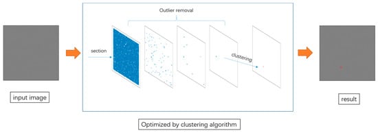
Figure 1.
The overall framework of the proposed method.
The contributions of this study can be summarized as follows:
- A model of an optical imaging system for dim-weak targets is established, and the multi-frame imaging performance of dim-weak targets post-disturbance is simulated.
- The detection problem of dim-weak targets is modeled as the problem of finding the center of the connected domain in graphics. The difference in energy distribution between the target and noise regions was exploited to realize the detection of dim-weak point targets.
- A new dim-weak point target detection method is proposed that is optimized via a clustering algorithm to address the difficulty in detecting dim-weak point targets with multi-frame superposition following the convergence of the target energy. It has good detection performance when the SNR is 1 dB.
2. Related Work
In this section, we focus on the relevant research in this field. Currently, the detection methods for dim targets primarily include traditional and deep-learning methods.
2.1. Traditional Method
2.1.1. Single-Frame Image Detection
In the single-frame image detection method, methods based on spatial filtering include least mean square filtering [13], maximum filtering [14], and local contrast measurement [15]. In recent years, several researchers have proposed improved methods such as multi-scale patch-based contrast measurement [16], weighted local difference measure [17], multi-scale relative local contrast measure [18], and local average gray difference measure [19]. However, most of these methods rely on the difference in gray scale between the target and background, which decreases when the target becomes faint; hence, detection cannot be achieved accurately. Furthermore, the methods based on transform domain filtering primarily include wavelet transform [20], Fourier transform [21], and the IPI model [22]. However, these methods need to select the most suitable parameters based on experience or have strict requirements for data preprocessing, and hence, extremely faint targets cannot meet these applicable conditions owing to weak signals. Therefore, these methods do not function satisfactorily.
2.1.2. Multi-Frame Image Detection
The basic multi-frame image detection method is a differential method, such as the background subtraction method [23] and inter-frame difference method [24], which use the differences frame-to-frame for detection, with simple principles and fast processing. However, the detection performance decreases sharply when the background changes or fluctuates. Most conventional multi-frame filtering methods are based on strong prior knowledge of the target. For example, the optical flow method [25] assigns a velocity vector to each pixel and detects the target according to its variation. The particle filter method [26,27,28] uses the probability density of a set of random samples to estimate small targets. The multi-level matching method [29] sets multiple thresholds as the classification threshold and performs segmented and layered level-by-level matching. The three-dimensional matched filtering method [30] matches the target in the spatial and temporal domains according to its motion pattern. The dynamic programming method [31] designs the evaluation function according to the maximum probability criterion for detection. The detection performance of these methods decreases when the speed of the target is unknown, or the noise is significantly large for the target to be prominent enough.
2.2. Deep-Learning Methods
In recent years, owing to the rising wave of machine learning, many researchers are using CNNS to solve the problem of faint target detection. Common CNN-based deep-learning target detection methods include R-CNN [32], Fast R-CNN [33], Faster R-CNN [34], and YOLO [35]. However, considering that the spatial features of faint targets are not obvious, the information loss caused by multi-layer convolution and pooling leads to loss or even complete invisibility of the spatial features of faint targets. Therefore, the current classic target detection model is not effective in detecting dim-weak targets. Most current detection methods based on deep learning for faint targets are oriented to scenes where infrared small targets are treated as typical targets. For example, TBCnet [36] extracts small targets from infrared images and imposes semantic constraints on the targets to suppress background false alarms. MD vs. FA-GAN [37] utilizes adversarial generative networks to balance against missed detections and false alarms. CDME [38] treats small targets as noise and uses denoising self-encoders for detection. IRSTD-GAN [39] considers infrared small targets as a special type of noise that can be predicted based on the features learned by GAN. ACMnet [40] employs asymmetric context modulation to infrared small targets and uses spatial attention mechanisms to focus on small targets. ALCnet [41] uses the method of cyclic displacement of feature maps and modularizes the method of local contrast metrics into a parameter-free optimization network layer. DNAnet [42] combines a densely nested interaction and channel-spatial attention module. Most of these methods perform well on self-built infrared weak target datasets. Although these types of data occupy fewer pixels, the target is brighter compared to the background, and the local contrast and SNR are higher, which still has some drawbacks when applied to dark and weak targets. Therefore, it is necessary to develop a new method of dim-weak point target detection.
3. Proposed Methods
In this section, we introduce the imaging model of the dim-weak target optical system, describe the mathematical model and imaging process of each component, and introduce the multi-frame superposition method and its problems.
3.1. A Model of Optical Imaging System for Dim-Weak Targets
We consider the imaging process to be a linear process in both time and energy. In particular, the formation of each component is independent of each other, and the final imaging result comprises three components: background signal , target signal , and noise signal . The following is the image model definition for this study:
Considering a dark background, which is stable under a normal scenario, is set as constant in the experiment to minimize the influence of the initial environment on the target imaging, as shown in the following formula.
The imaging process of a point target can be considered using an array to down-sample the response of the point target after imaging and forming discrete gray values on the image [43]. According to the linear system response formula, the response of point target after passing through the optical system can be considered the convolution of point target and point spread function . Therefore, the following point-target response formula can be obtained:
The convolution of the point pixels and point spread function in optical imaging forms the point target response, which is discretely down-sampled by the array to form the final point target imaging. Figure 2 shows the imaging process of a point target. Before passing through the imaging system, the point target is represented by the prominent value on the point pixel, whereas after passing through the imaging system, the target presents a stepped distribution of grayscale values on the array.
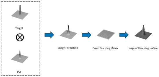
Figure 2.
Schematic of the imaging process: point target and point diffusion function convolution after array down-sampling to form the final imaging results.
The point spread function is a two-dimensional Gaussian-like model centered on the point pixel response value, and its essence is the spatial domain expression of the transfer function of the imaging system. In this simulation, the extended two-dimensional Gaussian function is used as the mathematical model of the point spread function, and the intensity of the target is set by controlling the values of , , and to constrain the spread range of the target. Therefore, the objective function is defined as follows:
3.2. Multi-Frame Superposition
In general, the weak signal of a single-frame image can be enhanced by extending the exposure time of the shooting device; however, this improvement is limited. When the exposure time reaches a critical value, the energy of the target no longer increases significantly, and when there is movement of the target, continuous exposure causes changes in the energy distribution of the target within the frame, resulting in smearing. Therefore, using the multi-frame superposition method to enhance the dim-weak point target data can break through the detection limit of the physical device and effectively improve the SNR of the target, thereby resulting in the convergence of the energy of the target, which is convenient for subsequent detection. Formula (5) represents the calculation formula for the power SNR, where represents the signal power, represents the noise power, represents the average of the target signal, and represents the standard deviation of the noise signal. After multi-frame superposition, the signal energy is also superimposed. As shown in Formula (6), indicates the signal after frames are superimposed, because the target signal remains unchanged. Thus, . Additionally, the noise of each frame is independent of each other, so . Thus, from Formulas (5) and (6), it can be proven that after superimposing the K frame image, the SNR can be increased by a factor of . However, because of the instability of the imaging system, the target produces random small movements on the imaging plane. The target randomly shifts for a short period of time near the center. In this new position, a new response value is generated according to the imaging system. After each frame is accumulated, the response value of multiple point targets is formed eventually, resulting in the energy accumulation error of multi-frame superposition. The target energy spreads in the neighborhood, making detection difficult. For this representation of the data, we propose a new detection method.
The actual imaging process faces many problems, such as platform jitter, instrument noise, light pollution, and atmospheric pollution that interfere with the imaging results. However, most interference factors can be avoided by certain methods, such as changing the shooting location and selecting a suitable shooting time. However, the slight jitter generated by the shooting platform and thermal noise brought by the instrument is unavoidable, having a significant impact on the detection. Therefore, this study analyzed the effects of these two types of interference on the target. In particular, the first type includes small movements of the target imaging brought by the instability of the imaging system, and the second type is interference from the thermal noise of the imaging system.
3.2.1. Type I Interference
This slight movement is generated by the shaking of the shooting equipment or relative movement of the object position on the imaging surface because of other influences in the imaging process. This movement is disordered and irregular and occurs simultaneously in both directions. In particular, we ignore the influence of these motions on the energy distribution of weak point objects within the frame, that is, the point objects can be considered to be stationary within the frame for extremely short shooting times. According to the above explanation, the disturbance suffered by the target conforms to a random Gaussian distribution, where is the number of superimposed frames and (, ) represents the offset of the target in two directions. The form is shown in Formula (7).
As shown in Figure 3, because the offset of the point target generates a new response at the new position, the superposition of the response values at multiple positions causes the responses of each point to mix with each other. Generally, the peak no longer appears at the original center point, multiple peaks appear, energy diffuses into nearby pixels, or image fragmentation occurs.
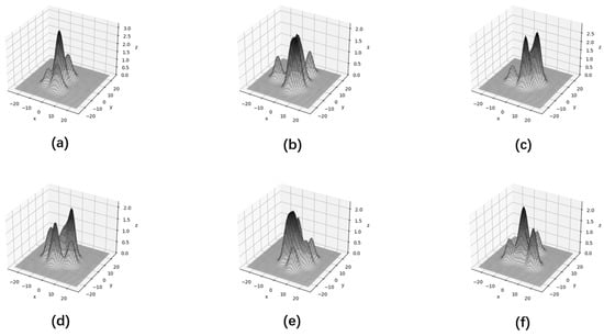
Figure 3.
Multi-frame superimposed point target imaging: (a,f) present a higher peak and some smaller peaks; (b,e) present a situation where the responses are mixed with each other; (c) presents two similar peaks; (d) presents a broken change model.
3.2.2. Type II Interference
Unlike bright targets with high SNR, targets with low energy and dim features have weakened resistance to noise, making them easily susceptible to noise. The target may be completely submerged or misshapen, ensuring that it is no longer a complete Gaussian-like shape because of contamination. As can be seen in Figure 4, as the SNR decreases, the target’s performance in the airspace becomes weaker. Because most of the noise brought by electronic instruments is thermal noise, which is a typical Gaussian white noise [44], it is used for simulation in this study.
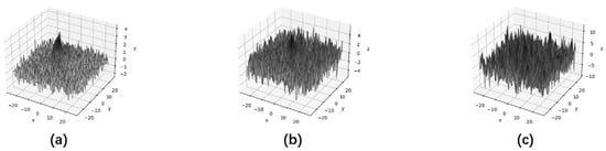
Figure 4.
Superposition of target and noise: the noise of (a–c) graphs gradually increases, and the SNR gradually decreases.
Through the superposition of the above two types of interference, it can be found that the current detection difficulties are mainly because of the weak energy of the target, being submerged by noise, losing significance in the space domain, and exhibiting faint features. In the process of multi-frame superposition, the target energy dispersion and fragmentation are caused by the target energy accumulation error owing to small movements.
To address the above problems, we propose a multi-frame superposition detection algorithm based on clustering optimization, which models faint target detection as a problem of finding the center of the connected domain in graphics and uses the difference between the distribution of the target area and noise to detect the target.
3.3. Detection Based on Optimized Clustering Algorithm
In order to solve the problem of the limitation of target space domain features, our solution is to convert the image into a scatter plot and combine the energy distribution difference feature of the target and noise on the image with the clustering algorithm for detection. Since the target follows a Gaussian distribution in the imaging system, a small, connected domain is projected onto the plane after dimensionality reduction, and the noise is random and often appears as some isolated points, and this difference can help us detect the target.
It can be derived from Formulas (8)–(10) that because the target satisfies the Gaussian distribution model; theoretically, when the specified is set, the set of , forms an ellipse centered on , under ideal circumstances; the energy values of the points inside the ellipse are higher than , and, therefore, there must exist an ellipse-like connected domain on the projection surface. Because the noise does not have this distribution feature, we use the difference of this characteristic to detect the target.
In the proposed method, the three-dimensional data are first reduced to two-dimensional data, and a projected scatter diagram is formed. Subsequently, the center point of the connected domain is calculated using the clustering method in machine learning. Finally, it is used as the original center point of the target energy distribution function for inspection. Each step is explained below.
For the faint target, after specifying the intensity range, screening the specific intensity size does not contribute to detection. More importantly, it should be clear whether there is a point that satisfies the intensity value. Through this method, the original three-dimensional data are downscaled into two dimensions, and hence, a two-dimensional scatter plot is obtained. Figure 5 below demonstrates processing under different SNR values. It can be seen that a difference in the distribution exists, although the target energy is weakened.
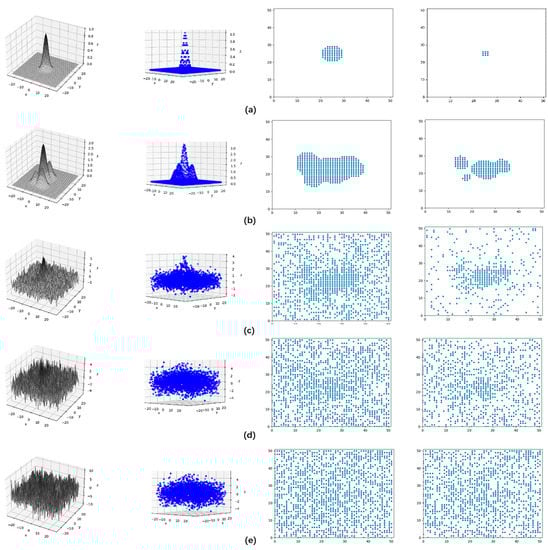
Figure 5.
Diagram of preprocessing under different conditions: (a) is the ideal imaging of a point target; (b) is the imaging of a point target after multi-frame superimposition; (c) has superimposed noise compared with (b); (d) has reduced SNR; (e) is pure noise.
The clustering method is an important technique of classification that divides the data into different clusters according to the given rules to generate significant similarities in the same cluster. Furthermore, the difference between the data of different clusters is as large as possible.
The k-means clustering algorithm, a division-based clustering method that uses distance as a rule for division, was used to solve the above problems. The process is as follows: First, we randomly selected K data objects in the given data as the initial K clusters . For the remaining points, we calculated the distance from the center point of each cluster according to the formula and compared each of them. We calculated the distance from a point to the center point of each cluster, adding the point to be classified to the cluster closest to the cluster center. Subsequently, the center of the new cluster was computed, and the amount of change from the last cluster was recorded for this center, which was iterated until all the data were traversed. For K-means, various distance calculation formulas can be used. Based on the experimental results, the Euclidean distance, Formula (11), was selected in this study. In this study, a single target is mainly used as the detection scenario, so the hyperparameter K is set to 1.
Because the noise model was Gaussian white noise, according to the nature of white noise, the first-order moments were constant, and the second-order moments were uncorrelated. Its amplitude distribution obeyed the Gaussian distribution, the power spectral density obeyed a uniform distribution, and the noise at any location at any moment was random with equal probability. Therefore, as shown in Formulas (12) and (13) where represents the variance of the noisy signal, indicates the standard deviation of the noisy signal. The cluster center calculated according to the Euclidean distance formula always appears in the center of the image, and it must be discriminated at this time.
Just like Figure 6, when the target center is in the same position, distinguishing the target center from the noise center becomes difficult. When the target center is not in the center of the image, the noise significantly impacts the clustering result of the target center if left untreated. Therefore, further manipulation of the data is needed to obtain a more accurate center position after forming the scatter plot.
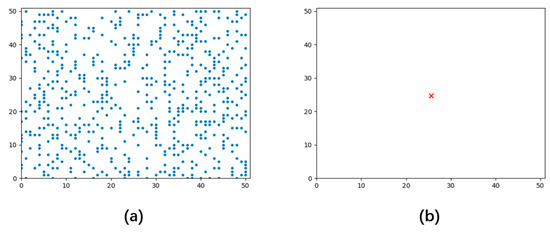
Figure 6.
The clustering center of noise: (a) is a noise scatter diagram; (b) is a clustering center, which is the image center.
According to the analysis in our study, there is a connected domain in the target area, but noise does not have this characteristic, so many randomly distributed unrelated points will be formed on the scatter plot. To minimize the impact of noise on the detection results, we removed isolated points from the scatterplot. We introduced the idea of an outlier removal method in point cloud data preprocessing. Points that do not have other points in the surrounding eight neighborhoods are defined as outliers. Figure 7 is a schematic of the outliers.
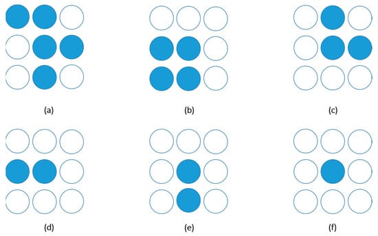
Figure 7.
Outliers: (a–e) show points with connected domains; (f) shows outliers.
In the experiment, in order to obtain better results, we adjusted the judgment criterion and experimented on the cases of 4-neighborhoods and 8-neighborhoods. We removed the data with different SNRs for 4-neighborhood outliers and 8-neighborhood outliers once, and the results are shown in Figure 8 and Figure 9. We found that selecting no other points in the 4-neighborhood as outliers removed more noise. Subsequently, an ablation experiment was performed to compare the effects of the two criteria on the detection results. From Table 1, it can be found that the improvement in the detection results when using four points as the judgment criterion is more obvious, so the isolated noise is removed in this method in subsequent experiments.
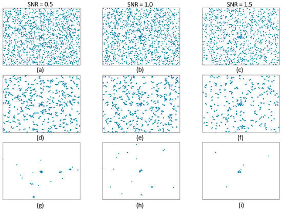
Figure 8.
Experimental results from 0.5 to 1.5 dB: (a–c) are the original images. (d–f) are the results of 8-neighbour. (g–i) the results of 4-neighbour.
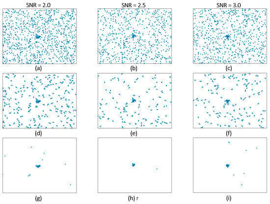
Figure 9.
Experimental results from 2.0 to 3.0 dB: (a–c) are the original images. (d–f) are the results of 8-neighbour. (g–i) the results of 4-neighbour.

Table 1.
Comparative experimental results of 4-neighborhoods and 8-neighborhoods.
Figure 10 shows the processing results of different SNRs. When the SNR of the target is high, it can be seen that the distribution characteristics of the target are significant. Although there is the first type of interference, there are still many aggregation points near the target point. The processed scatter diagram can effectively leave the aggregation point-connected domain. However, as the SNR of the target decreases, the influence of the background noise on the target becomes greater, and the energy distribution of the target is clearly diffused because of the slight movement of the target. Additionally, the point distribution in the target area changes. When the SNR drops to a very low level, the joint effect of the two kinds of interference on the target makes the original distribution characteristics of the target no longer obvious, and the noise and the target are mixed together, making it difficult to distinguish between them.
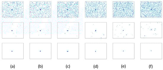
Figure 10.
Processing diagrams under different SNRs: (a–f) Gradual decrease in SNR.
4. Experiment and Analysis
This section describes the evaluation metrics and shows the performance of our algorithm on the simulated and real data, as well as comparative experiments with other methods.
4.1. Evaluation Metrics
We introduced evaluation metrics to evaluate the performance of the proposed algorithm. In this experiment, because the target is small and the energy is weak, LSNR is used to measure the difference between the target and local background. It is defined as the average energy of the target region minus the average energy of the background multiplied by the inverse of the standard deviation of the background. It is calculated by Formula (14). Among them, and represent the average values of the target energy and background energy, respectively, and represents the standard deviation of the background energy. The background area was calculated with the target as the center, and the target size was expanded outward three times to ensure the calculation accuracy.
For object detection, the most commonly used evaluation criteria are precision and recall, which indicate the probability of correctly predicting a positive sample in a positive prediction and the probability of correctly predicting a positive sample in a correctly classified sample, respectively. These three indicators are defined as follows:
To evaluate the detection ability of different methods for dim-weak targets with an SNR of 1 dB, the detection probability and false alarm rate are introduced as the evaluation indicators of model detection performance. represents the proportion of the number of detected targets to the actual number of targets, and represents the proportion of small targets that are falsely detected in all images. The indicators are defined as follows:
4.2. Simulation Data
In this section, we focus on the performance of the proposed method with the simulation data. The image size set in the simulation was 501 × 501; the target size was set to 5 × 5 pixels. In our experiment, the gray value of the background is set to 50. The noise was set as Gaussian white noise with a mean of 0 and standard deviation of 1. The target position was set randomly on the image, and random motion was generated on the X and Y axes. The overlay frame number was 10 frames.
Since this study is aimed at the detection of dim-weak targets, we only discuss the situation where the target SNR is relatively low, and our method is applicable to the target energy being greater than the background energy, so the SNR needs to be greater than 0 dB, so we set the minimum SNR to 0.5 dB. Therefore, in the simulation, the main target SNR interval was set as 3–0.5 dB. In order to determine the limit of detection, more specifically, there are 14 sets of data with different SNRs. We set six intervals of 0.5 between 3 and 0.5 dB to observe the performance of our method when the SNR of the target continues to decrease. To get a closer look at how our method performs on low-SNR targets, we add more test points between 1.5 and 0.5 dB and set the SNR of the target at 0.1 intervals. In each interval, 1000 sets of data were simulated, for a total of 14,000 sets of data, and the following simulation results were obtained. In Figure 11, the gray image represents the generated simulation data, and the blue circle represents the target location. Figure 12 represents 3D views of the grayscale value near the target. The upper right corner of each image is marked with the SNR value corresponding to the data.
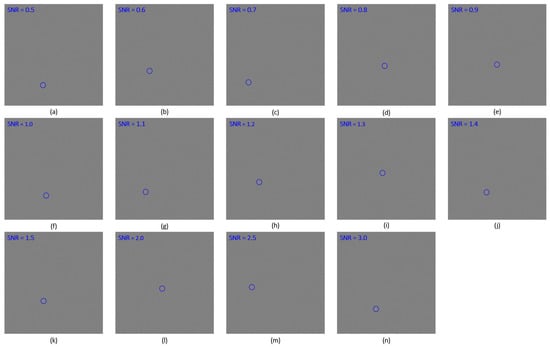
Figure 11.
Schematic diagram of 14 sets of simulation data: (a–n) are the original images with different SNRs, the blue circle represents the target location.
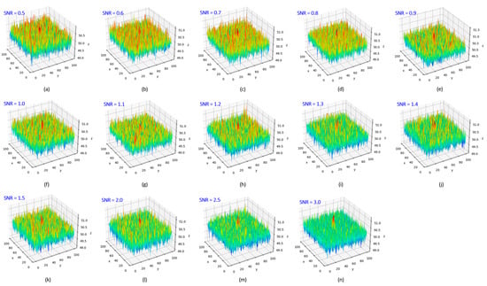
Figure 12.
Three-dimensional view of the grayscale value near the target: (a–n) are the 3D views with different SNRs.
From Table 2 and Figure 13, it can be concluded that with the decrease in SNR, the precision, recall, and accuracy all gradually decrease. There is a large decrease between 1.5 and 0.5 dB. What can be obtained by observing Table 3 is that when the SNR is above 1 dB, all three are above 80%. When the SNR is lower than 1 dB, the detection effect drops significantly, but when the SNR is 0.5 dB, an accuracy rate of 81.9% can still be obtained. Overall, the results show that this method has high detection accuracy and is even suitable for low-SNR dim-weak target detection.
Table 2.
Test results with an interval of 0.5 dB.
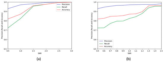
Figure 13.
The detection effect of this method under different SNRs. (a) is the result from 0.5 to 3 dB. (b) is the result from 0.5 to 1.5 dB.
Table 3.
Test results with an interval of 0.1 dB.
In addition, we also calculated the running time of this method in the above 14 sets of data with different SNRs. The results are shown in Table 4 and Table 5, and it can be concluded that the running time of our method is not affected by the difference in SNR, and the performance is relatively stable. However, our algorithm is not optimized in code, and the parallelism of algorithm implementation will be considered in the future.
Table 4.
Running time at 0.5–1.1 dB.
Table 5.
Running time at 1.2–3 dB.
4.3. Comparative Experiment
To test the superiority of this method, several representative methods were compared. We selected nine representative methods for comparison: multi-scale patch-based contrast measure (MPCM) [16], local intensity and gradient properties (LIG) [45], local contrast method utilizing a tri-layer (TLLCM) [46], absolute directional mean difference algorithm (ADMD) [47], weighted strengthened local contrast measure (WSLCM) [48], absolute average gray difference (AAGD) [49], self-regularized weighted sparse model (SRWS) [50], nonconvex tensor low-rank approximation (NTLA) [51], and self-adaptive and non-local patch-tensor (ANLPT) [52]. All experiments were run using the same workstation with a 3.20 GHz Intel Core i9-12900K CPU. The parameters selected for each method are listed in Table 6.
Table 6.
Summary of parameters.
4.3.1. Comparison of Simulation Data
The simulation test data used were the simulation data used in the experiments in Section 4.2. Figure 14 shows the ROC curves of different methods on simulated data with different SNRs. The closer the curve is to the upper-left corner, the better the performance. We calculated the area under the ROC curve (AUC) corresponding to the method shown in Table 7, Table 8 and Table 9; the higher the AUC, the better the detection performance of the method.
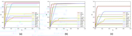
Figure 14.
ROC curves of different methods of simulation data. (a) is the result of a SNR of 1.5 dB. (b) is the result of a SNR of 1 dB. (c) is the result of a SNR of 0.5 dB.
Table 7.
AUC of different methods when the SNR is 1.5 dB.
Table 8.
AUC of different methods when the SNR is 1 dB.
Table 9.
AUC of different methods when the SNR is 0.5 dB.
In Figure 14, it is found that as the SNR of the simulated data decreases, the detection of all methods decreases to varying degrees. MPCM, ADMD, and AAGD have large advantages over the other compared methods, especially if the SNR is greater than or equal to 1 dB. Of the three, AAGD has a higher false alarm rate, ADMD has a lower detection probability, and MPCM is the best-performing method of the three. The detection capability of the TLLCM method is sensitive to a decrease in SNR. The remaining methods are no longer effective at a SNR of 1.5 dB and are less capable of detecting low SNR targets. In our experiments, with all methods compared, the LIG method had the highest false alarm rate, and the WSLCM method had the lowest detection probability. When the SNR drops to 0.5 dB, the performance degradation of all methods is more pronounced. Figure 14 and Table 7, Table 8 and Table 9 show that our method has an advantage in the comparison of the detection performance in all three data sets, indicating that our method has better detection capability for low SNR targets in the simulation situation.
Combined with the previous analysis, we find that although the performance of our method decreases when the SNR is lower than 1.5 dB, and when the SNR is 1 dB, various indicators can still be at a high level. Figure 15 shows some test results of all methods when the SNR is 1 dB. The blue circle indicates the ground truth on the original image, the blue box indicates that the predicted value on the resulting plot is consistent with the true value and the target is correctly detected, the orange box indicates that the target is detected but does not match the true value, and no box indicates that no target is detected. Table 10 compares the run times of the different methods.
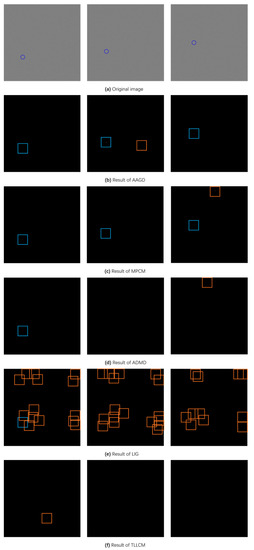
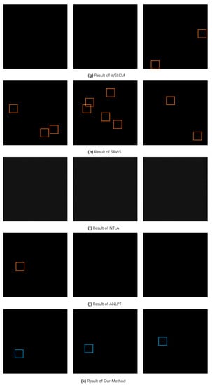
Figure 15.
Comparison experiment results diagram: Partial detection results for targets with a SNR of 1 dB.
Table 10.
Running time of different methods when the SNR is 1 dB.
From Figure 14 and Figure 15, when the SNR is 1 dB, the WSLCM method often cannot detect the target and, therefore, loses its applicability. The TLLCM, NTLA, and ANLPT methods have a very low detection rate for the target, and the detection effects of TLLCM, NTLA, and ANLPT methods are also relatively poor. When the difference between the background and the target is not clear, it is difficult for the LIG and SRWS methods to distinguish the two from the target and the background noise. The outstanding value is detected as a target, and many false detections can be seen in Figure 15. Although the ADMD method can detect the target well, the performance is not stable, and sometimes the edge of the image and the point with a sharp gradient change are used as the target detection. An example is shown in Figure 15d. For the MPCM and AAGD methods, the detection performance of the method is better, but the false alarm rate is slightly higher than the method in this study. As can be seen from the graph in Figure 14 and Table 7, Table 8 and Table 9, the method proposed in this study outperforms other methods on ROC and achieves the highest AUC, which proves the superiority of the method in this paper. Although our algorithm has advantages in detection capabilities, our algorithm adds complexity compared to some basic algorithms and, therefore, requires a longer run time. In the future, we will work on optimizing the algorithm process to speed up the running time.
4.3.2. Comparison of Real Data
In order to show the applicability of our method in real scenarios, we selected six sets of data for testing. The dataset comes from the public dataset [53], and the experimental scene includes typical detection backgrounds, such as sea surface, sky, and clouds, and each scene is a sequence. Because the targets in the data have the nature of motion and the background is relatively complex, the SNR of the picture under each scene sequence is not the same. In order to ensure the readability of the experimental results, we calculated the SNR of all images, screened out the images with a low SNR in the same sequence in different scenes, and recombined them into the dataset we used for testing so as to ensure that each set of data has a similar image composition and the SNR is within the specified interval. The grouping experiment is carried out according to the different SNRs, and the details of the experimental data are shown in Table 11 below.
Table 11.
Detail of real datasets.
In Figure 16, Figure 17 and Figure 18, we show part of the real data experiment result map; the ground truth in the original image is marked with a blue circle, and the detection value is marked with a red box. In order to increase the visualization of the results, we also draw three-dimensional views of the detection results. We also list the SNR corresponding to the image. Since there are many pictures, we divide the resulting plot into three figures. Then we listed the ROC curves of all methods on the six sets of data in Figure 19 and calculated the AUC value, and the results are shown in Table 12.
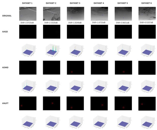
Figure 16.
Resulting diagrams from the comparison experiment: AAGD, ADMD, and ANLPT.
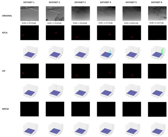
Figure 17.
Resulting diagrams from the comparison experiment: NTLA, LIG, and MPCM.
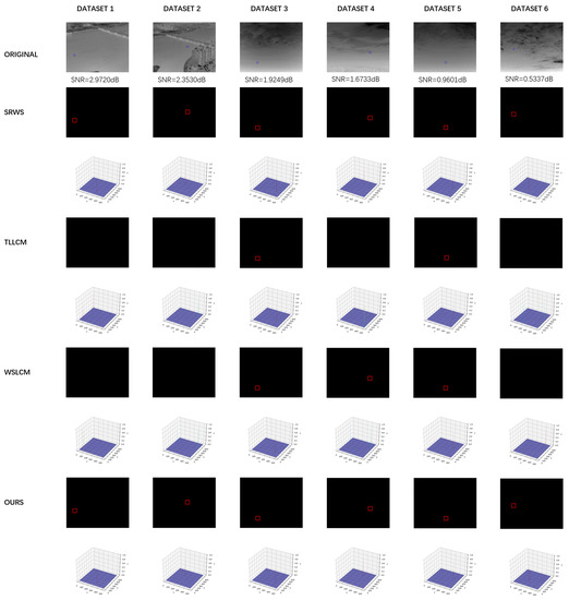
Figure 18.
Resulting diagrams from the comparison experiment: SRWS, TLLCM, WSLCM, and Our method.
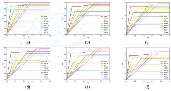
Figure 19.
ROC curves of different methods on real datasets. (a) is the result of Dataset 1. (b) is the result of Dataset 2. (c) is the result of Dataset 3. (d) is the result of Dataset 4. (e) is the result of Dataset 5. (f) is the result of Dataset 6.
Table 12.
AUC of different methods with real datasets.
As shown in the results in Figure 19, in the real scenario, the performance of all methods degrades to varying degrees with a decrease in the SNR. Our method can stably detect targets when the SNR is greater than 1 dB, but the detection performance decreases significantly when the SNR is 0.5 dB. Although the AAGD method shows good detection ability on simulated data, it performs poorly on real data, and when some bright areas appear in the background, it will be output as a target, resulting in a lot of false alarms and missed detections. Although the MPCM method produces fewer false positives than the AAGD method, it still does not achieve the desired results. The ADMD method can be effectively detected at high SNR, but with a decrease in SNR, the detection rate decreases rapidly. ANLPT, NTLA, and LIG methods can complete the detection of targets well, but at the same time, they will be accompanied by a high false alarm rate; among the three, the LIG method can obtain the best effect. Compared with these three methods, the false alarm rate of WSLCM and SRWS methods has improved, but the detection rate cannot be maintained at a high level. Among all the comparison methods, the TLLCM method has the best test results, and our method has certain advantages in false alarm rate and detection rate compared to it. In Table 10, our method also obtained the highest AUC value.
5. Conclusions
This study proposes a multi-frame superposition detection method for dim-weak targets based on the optimized clustering algorithm to solve the problem of weak energy of the faint target and the energy accumulation error and noise interference in the process of multi-frame superposition, which renders the SNR of the target lower and is difficult to detect. This method combines the energy distribution characteristics of the target with the clustering method. First, we established a simulated optical system imaging model to simulate the tiny motion and noise in multi-frame imaging and analyzed the imaging feature of the faint target. Subsequently, we transformed the problem of dim-weak point target detection into the problem of identifying the center of the connected domains in graphics. Furthermore, to extract the target characteristics, we used the outlier removal method to leave a relatively pure connected domain, and the data were passed through the clustering model for calculation. Finally, experiments on simulated data and real data demonstrated that this method can effectively detect dim and small targets with low SNR, as the accuracy rate reaches 87.1% when the SNR is 1 dB. The comparison experiments with other methods in real scenarios show that this method has better detection performance. However, this method still has limitations when SNR is further reduced, especially at less than 0.5 dB, considering the target is significantly affected by noise, resulting in energy dispersion and entanglement. The main reason is that this paper uses a single feature for detection. In future research, we hope to focus on the addition of multiple features to handle this issue.
Author Contributions
Conceptualization, C.X. and W.Z.; methodology, C.X.; software, C.X.; validation, C.X., E.Z. and W.Z.; resources, W.Z., Z.Y., X.P. and W.N.; data curation, C.X.; writing—original draft preparation, C.X.; writing—review and editing, C.X., E.Z. and W.Z.; visualization, C.X.; supervision, W.Z. project administration, W.Z., Z.Y., X.P. and W.N. All authors have read and agreed to the published version of the manuscript.
Funding
This work was supported by the Strategic Priority Research Program of China Academy of Sciences (Grant No. XDA17040525), and the Strategic Priority Research Program on Space Sciences. Chinese Academy of Sciences, grant number XDA15014900.
Data Availability Statement
Not applicable.
Conflicts of Interest
The authors declare no conflict of interest.
References
- Wirnsberger, H.; Baur, O.; Kirchner, G. Space debris orbit prediction errors using bi-static laser observations. Case study: ENVISAT. Adv. Space Res. 2015, 55, 2607–2615. [Google Scholar] [CrossRef]
- Dawson, J.A.; Bankston, C.T. Space debris characterization using thermal imaging systems. In Proceedings of the Advanced Maui Optical and Space Surveillance Technologies Conference, Wailea, Maui, HI, USA, 14–17 September 2010. [Google Scholar]
- Prasad, D.K.; Rajan, D.; Rachmawati, L.; Rajabally, E.; Quek, C. Video processing from electro-optical sensors for object detection and tracking in a maritime environment: A survey. IEEE Trans. Intell. Transport. Syst. 2017, 18, 1993–2016. [Google Scholar] [CrossRef]
- Chen, X.; Xu, W.; Tao, S.; Gao, T.; Feng, Q.; Piao, Y. Total Variation Weighted Low-Rank Constraint for Infrared Dim Small Target Detection. Remote Sens. 2022, 14, 4615. [Google Scholar] [CrossRef]
- Liu, C.; Wang, H. Research on infrared dim and small target detection algorithm based on low-rank tensor recovery. J. Syst. Eng. Electron. 2023, 1–12. [Google Scholar] [CrossRef]
- Bai, X.; Zhang, S.; Du, B.; Liu, Z.; Jin, T.; Xue, B.; Zhou, F. Survey on Dim Small Target Detection in Clutter Background: Wavelet, Inter-Frame and Filter Based Algorithms. Procedia Eng. 2011, 15, 479–483. [Google Scholar] [CrossRef]
- Zscheile, J.; Wagner, P.; Lorbeer, R.A.; Guthier, B. Synthetic tracking for orbital object detection in LEO. In Proceedings of the 1st NEO and Debris Detection Conference, Darmstadt, Germany, 22–24 January 2019; Available online: https://conference.sdo.esoc.esa.int/proceedings/neosst1/paper/399 (accessed on 13 June 2022).
- Wei, P.; Zeidler, J.; Ku, W. Analysis of multi-frame target detection using pixel statistics. IEEE Trans. Aerosp. Electron. Syst. 1995, 31, 238–246. [Google Scholar] [CrossRef]
- Wei, Z.; Cong, M.; Wang, L. Algorithms for optical weak small targets detection and tracking: Review. In Proceedings of the International Conference on Neural Networks and Signal Processing, Nanjing, China, 14–17 December 2003. [Google Scholar] [CrossRef]
- Hou, W.; Sun, X.; Shang, Y.; Yu, Q. Present State and Perspectives of Small Infrared Targets Detection Technology. Infrared Technol. 2015, 37, 1–10. [Google Scholar]
- Wang, H.; Dong, H.; Zhou, Z. Review on Dim Small Target Detection Technologies in Infrared Single Frame Images. Laser Optoelectron. Prog. 2019, 56, 080001. [Google Scholar] [CrossRef]
- Xia, J.Z.; Liu, Y.H.; Len, Y.G.; Ge, J.T. Analysis of Methods of Weak Signal Detection. Noise Vib. Control 2011, 31, 156–161. [Google Scholar]
- Lv, P.Y.; Sun, S.L.; Lin, C.Q.; Liu, G.R. Space moving target detection and tracking method in complex background. Infrared Phys. Technol. 2018, 91, 107–118. [Google Scholar] [CrossRef]
- Singla, N. Motion detection based on frame difference method. Int. J. Inf. Comput. Technol. 2014, 4, 1559–1565. [Google Scholar]
- Chen, C.L.P.; Li, H.; Wei, Y.; Xia, T.; Tang, Y.Y. A local contrast method for small infrared target detection. IEEE Trans. Geosci. Remote Sens. 2013, 52, 574–581. [Google Scholar] [CrossRef]
- Wei, Y.; You, X.; Li, H. Multiscale patch-based contrast measure for small infrared target detection. Pattern Recognit. 2016, 58, 216–226. [Google Scholar] [CrossRef]
- Deng, H.; Sun, X.; Liu, M.; Ye, C.; Zhou, X. Small infrared target detection based on weighted local difference measure. IEEE Trans. Geosci. Remote Sens. 2016, 54, 4204–4214. [Google Scholar] [CrossRef]
- Han, J.; Liang, K.; Zhou, B.; Zhu, X.; Zhao, J.; Zhao, L. Infrared small target detection utilizing the multiscale relative local contrast measure. IEEE Geosci. Remote Sens. Lett. 2018, 15, 612–616. [Google Scholar] [CrossRef]
- Xie, F.; Dong, M.; Wang, X.; Yan, J. Infrared Small-Target Detection Using Multiscale Local Average Gray Difference Measure. Electronics 2022, 11, 1547. [Google Scholar] [CrossRef]
- Wang, H.; Xin, Y. Wavelet-based contourlet transform and kurtosis map for infrared small target detection in complex background. Sensors 2020, 20, 755. [Google Scholar] [CrossRef]
- Ren, K.; Song, C.; Miao, X.; Wan, M.; Xiao, J.; Gu, G.; Chen, Q. Infrared small target detection based on non-subsampled shearlet transform and phase spectrum of quaternion Fourier transform. Opt. Quantum. Electron. 2020, 52, 1–15. [Google Scholar] [CrossRef]
- Gao, C.; Meng, D.; Yang, Y.; Wang, Y.; Zhou, X.; Hauptmann, A.G. Infrared patch-image model for small target detection in a single image. IEEE Trans. Image Process. 2013, 22, 4996–5009. [Google Scholar] [CrossRef]
- Zivkovic, Z. Improved adaptive Gaussian mixture model for background subtraction. In Proceedings of the 17th International Conference on Pattern Recognition, Cambridge, UK, 26 August 2004. [Google Scholar] [CrossRef]
- Liu, X.; Jin, X. Algorithm for object detection and tracking combined on four inter-frame difference and optical flow methods. Opto-Electron. Eng. 2018, 45, 170665. [Google Scholar] [CrossRef]
- Hossen, M.K.; Tuli, S.H. A surveillance system based on motion detection and motion estimation using optical flow. In Proceedings of the 5th International Conference on Informatics, Electronics and Vision (ICIEV), Dhaka, Bangladesh, 13–14 May 2016. [Google Scholar] [CrossRef]
- Chang, L.; Liu, Z.; Wang, S. Tracking of infrared radiation dim target based on mean-shift and particle filter. In Proceedings of the 2014 IEEE Chinese Guidance, Navigation and Control Conference, Yantai, China, 8–10 August 2014; pp. 671–675. [Google Scholar] [CrossRef]
- Tian, M.; Chen, Z.; Wang, H.; Liu, L. An Intelligent Particle Filter for Infrared Dim Small Target Detection and Tracking. IEEE Trans. Aerosp. Electron. Syst. 2022, 58, 5318–5333. [Google Scholar] [CrossRef]
- Huo, Y.; Chen, Y.; Zhang, H.; Zhang, H.; Wang, H. Dim and Small Target Tracking Using an Improved Particle Filter Based on Adaptive Feature Fusion. Electronics 2022, 11, 2457. [Google Scholar] [CrossRef]
- Villeneuve, P.V.; Fry, H.A. Improved matched-filter detection techniques. In Imaging Spectrometry V; SPIE: Bellingham, WA, USA, 1999; Volume 3753, pp. 278–285. [Google Scholar]
- Reed, I.S.; Gagliardi, R.M.; Stotts, L.B. Optical moving target detection with 3-D matched filtering. IEEE Trans. Aerosp. Electron. Syst. 2002, 24, 327–336. [Google Scholar] [CrossRef]
- Fu, J.; Zhang, H.; Luo, W.; Gao, X. Dynamic programming ring for point target detection. Appl. Sci. 2022, 12, 1151. [Google Scholar] [CrossRef]
- Girshick, R.; Donahue, J.; Darrell, T.; Malik, J. Rich feature hierarchies for accurate object detection and semantic segmentation. In Proceedings of the IEEE Conference on Computer Vision and Pattern Recognition, Columbus, OH, USA, 23–28 June 2014. [Google Scholar] [CrossRef]
- Girshick, R. Fast R-CNN. In Proceedings of the IEEE International Conference on Computer Vision (ICCV), Santiago, Chile, 7–13 December 2015; pp. 1440–1448. [Google Scholar] [CrossRef]
- Ren, S.; He, K.; Girshick, R.; Sun, J. Faster R-CNN: Towards real-time object detection with region proposal networks. IEEE Trans. Pattern Anal. Mach. Intell. 2017, 39, 1137–1149. [Google Scholar] [CrossRef] [PubMed]
- Redmon, J.; Divvala, S.; Girshick, R.; Farhadi, A. You only look once: Unified, real-time object detection. In Proceedings of the IEEE Conference on Computer Vision and Pattern Recognition, Las Vegas, NV, USA, 27–30 June 2016. [Google Scholar] [CrossRef]
- Zhao, M.; Cheng, L.; Yang, X.; Feng, P.; Liu, L.; Wu, N. TBC-Net: A Real-Time Detector for Infrared Small Target Detection Using Semantic Constraint. arXiv 2019, arXiv:2001.05852. [Google Scholar]
- Wang, H.; Zhou, L.; Wang, L. Miss Detection vs. False Alarm: Adversarial Learning for Small Object Segmentation in Infrared Images. In Proceedings of the International Conference on Computer Vision, Seoul, Republic of Korea, 27 October–2 November 2019. [Google Scholar] [CrossRef]
- Shi, M.; Wang, H. Infrared dim and small target detection based on denoising autoencoder network. Mob. Netw. Appl. 2020, 25, 1469–1483. [Google Scholar] [CrossRef]
- Zhao, B.; Wang, C.; Fu, Q.; Han, Z. A novel pattern for infrared small target detection with generative adversarial network. IEEE Trans. Geosci. Remote Sens. 2021, 59, 4481–4492. [Google Scholar] [CrossRef]
- Dai, Y.; Wu, Y.; Zhou, F.; Barnard, K. Asymmetric Contextual Modulation for Infrared Small Target Detection. In Proceedings of the IEEE/CVF Winter Conference on Applications of Computer Vision (WACV), Waikoloa, HI, USA, 3–8 January 2021. [Google Scholar] [CrossRef]
- Dai, Y.; Wu, Y.; Zhou, F.; Barnard, K. Attentional local contrast networks for infrared small target detection. IEEE Trans. Geosci. Remote Sens. 2021, 59, 9813–9824. [Google Scholar] [CrossRef]
- Li, B.; Xiao, C.; Wang, L.; Wang, Y.; Lin, Z.; Li, M.; An, W.; Guo, Y. Dense Nested Attention Network for Infrared Small Target Detection. IEEE Trans. Image Process. 2022, 32, 1745–1758. [Google Scholar] [CrossRef]
- Lei, Z.; Xin, Y.; Yi’nan, C.; Jixiang, Y. Object detection method based on generalized likelihood ratio tests method in photon images. Acta Opt. Sin. 2010, 30, 91–96. [Google Scholar] [CrossRef]
- Thompson, M. Intuitive Analog Circuit Design, 2nd ed.; Newnes: Oxford, UK, 2014; pp. 617–643. [Google Scholar] [CrossRef]
- Zhang, H.; Zhang, L.; Yuan, D.; Chen, H. Infrared small target detection based on local intensity and gradient properties. Infrared Phys. Technol. 2018, 89, 88–96. [Google Scholar] [CrossRef]
- Han, J.; Moradi, S.; Faramarzi, I.; Liu, C.; Zhang, H.; Zhao, Q. A Local Contrast Method for Infrared Small-Target Detection Utilizing a Tri-Layer Window. IEEE Geosci. Remote Sens. Lett. 2020, 17, 1822–1826. [Google Scholar] [CrossRef]
- Moradi, S.; Moallem, P.; Sabahi, M.F. Fast and robust small infrared target detection using absolute directional mean difference algorithm. Signal Process. 2020, 177, 107727. [Google Scholar] [CrossRef]
- Han, J.; Moradi, S.; Faramarzi, I.; Zhang, H.; Zhao, Q.; Zhang, X.; Li, N. Infrared small target detection based on the weighted strengthened local contrast measure. IEEE Geosci. Remote Sens. Lett. 2021, 18, 1670–1674. [Google Scholar] [CrossRef]
- Deng, H.; Sun, X.; Liu, M.; Ye, C.; Zhou, X. Infrared small-target detection using multiscale gray difference weighted image entropy. IEEE Trans. Aerosp. Electron. Syst. 2016, 52, 60–72. [Google Scholar] [CrossRef]
- Zhang, T.; Peng, Z.; Wu, H.; He, Y.; Li, C.; Yang, C. Infrared small target detection via self-regularized weighted sparse model. Neurocomputing 2020, 420, 124–148. [Google Scholar] [CrossRef]
- Liu, T.; Yang, J.; Li, B.; Xiao, C.; Sun, Y.; Wang, Y.; An, W. Nonconvex Tensor Low-Rank Approximation for Infrared Small Target Detection. IEEE Trans. Geosci. Remote Sens. 2022, 60, 1–18. [Google Scholar] [CrossRef]
- Zhang, Z.; Ding, C.; Gao, Z.; Xie, C. ANLPT: Self-Adaptive and Non-Local Patch-Tensor Model for Infrared Small Target Detection. Remote Sens. 2023, 15, 1021. [Google Scholar] [CrossRef]
- Sun, X.; Guo, L.; Zhang, W.; Wang, Z.; Hou, Y.; Li, Z.; Teng, X. A dataset for small infrared moving target detection under clutter background. Sci. Data Bank 2022. [Google Scholar] [CrossRef]
Disclaimer/Publisher’s Note: The statements, opinions and data contained in all publications are solely those of the individual author(s) and contributor(s) and not of MDPI and/or the editor(s). MDPI and/or the editor(s) disclaim responsibility for any injury to people or property resulting from any ideas, methods, instructions or products referred to in the content. |
© 2023 by the authors. Licensee MDPI, Basel, Switzerland. This article is an open access article distributed under the terms and conditions of the Creative Commons Attribution (CC BY) license (https://creativecommons.org/licenses/by/4.0/).