Article

Improving the Spatial Prediction of Soil Organic Carbon Content Using Phenological Factors: A Case Study in the Middle and Upper Reaches of Heihe River Basin, China

1
College of Earth Sciences, Chengdu University of Technology, Chengdu 610059, China
2
State Key Laboratory of Soil and Sustainable Agriculture, Institute of Soil Science, Chinese Academy of Sciences, Nanjing 210008, China
*
Author to whom correspondence should be addressed.
Remote Sens. 2023, 15(7), 1847; https://doi.org/10.3390/rs15071847
Submission received: 17 January 2023 / Revised: 18 March 2023 / Accepted: 28 March 2023 / Published: 30 March 2023

Abstract

:
The accurate mapping of soil organic carbon (SOC) distribution is important for carbon sequestration and land management strategies, contributing to mitigating climate change and ensuring agricultural productivity. The Heihe River Basin in China is an important region that has immense potential for SOC storage. Phenological variables are effective indicators of vegetation growth, and hence are closely related to SOC. However, few studies have incorporated phenological variables in SOC prediction, especially in alpine areas such as the Heihe River Basin. This study used random forest (RF) and extreme gradient boosting (XGBoost) to study the effects of phenological variables (e.g., Greenup, Dormancy, etc.) obtained from MODIS (i.e., Moderate Resolution Imaging Spectroradiometer) product (MCD12Q2) on SOC content prediction in the middle and upper reaches of Heihe River Basin. The current study also identified the dominating variables in SOC prediction and compared model performance using a cross validation procedure. The results indicate that: (1) when phenological variables were considered, the R 2 (coefficient of determination) of RF and XGBoost were 0.68 and 0.56, respectively, and RF consistently outperforms XGBoost in various cross validation experiments; (2) the environmental variables MAT, MAP, DEM and NDVI play the most important roles in SOC prediction; (3) the phenological variables can account for 32–39% of the spatial variability of SOC in both the RF and XGBoost models, and hence were the most important factor among the five categories of predictive variables. This study proved that the introduction of phenological variables can significantly improve the performance of SOC prediction. They should be used as indispensable variables for accurately modeling SOC in related studies.

1. Introduction

Soil carbon is the largest carbon pool in the terrestrial ecosystem, which has a significant influence on global climate change and agricultural productivity [1]. Soil organic carbon (SOC), as an important component of the soil carbon pool, serves as an important indicator of soil fertility and soil nutrient structure. Consequently, it plays a crucial role in measuring soil quality [2]. Accurately predicting SOC can provide data support for implementing effective soil carbon sequestration strategies, guide land management decisions and ultimately benefit mitigating climate change and preserving soil health [3,4,5].
A variety of methods have been used for SOC prediction, which can be typically grouped into three categories: (i) estimation based on soil profile data, (ii) estimation using spatial interpolation algorithms, and (iii) digital soil mapping (DSM) based on soil-landscape models. At the early stage, most studies firstly estimate average carbon density based on soil profiles and then obtain carbon content using the area ratio of different soil types and vegetation types [6,7]. However, due to the high variability of soil carbon content, the area estimation of different soil types or vegetation types typically varies when using different references [8]. Therefore, the resulting SOC content is subject to uncertainty. Estimation of SOC using spatial interpolation algorithms (e.g., kriging, inverse distance weighting, etc.) is affected by the quantity and configuration of sample points [9,10]. A reliable estimation typically requires the points be representative and evenly distributed across the region [10]. However, sampling points in hard-to-reach areas are usually sparse, resulting in estimations that are associated with high levels of uncertainty. McBratney [11] suggested that soil is the end product of both natural and anthropogenic processes that involve various factors such as terrain, climate, parent material and human activities. These factors combined are commonly referred to as the “soil-landscape model” [12,13,14]. Accordingly, DSM based on the soil-landscape model has been proposed for modeling soil properties. It has become the mainstream method for effectively predicting SOC content. Various studies have demonstrated the effectiveness of the method based on soil-landscape model and claimed that its performance is greatly influenced by the selection of environmental variables (e.g., elevation, slope, mean annual precipitation) and prediction models [15,16,17]. Therefore, how to determine a suitable set of environmental variables and an appropriate model for the area under study has become the key to achieving good performance in SOC prediction.
Remote sensing techniques have recently gained widespread acceptance in the inversion of physical parameters pertaining to the Earth’s surface landscape. This practice provides a new perspective and additional data sources for SOC prediction [18,19]. It is the most common practice to construct a vegetation index (e.g., normalized difference vegetation index, enhanced vegetation index) from remote sensing images, and further use them to predict SOC combined with other environmental factors. For example, Zhang [20] found that monthly NDVI data played an important role in SOC prediction in plain areas. Considering that soil and vegetation interact over a long period, the factors derived from remote sensing data with long time series can better capture the impact of vegetation changes on SOC, which is usually represented as “phenological variables” [21,22]. Phenological variables can indicate the periodic growth of vegetation, which indirectly influence SOC by reflecting vegetation productivity [23,24]. For example, delayed spring warming may lead to a shorter period of plant carbon uptake, resulting in decreased vegetation productivity. In contrast, a delayed hot summer can reduce the organic carbon consumed by soil respiration, leading to increased carbon storage as more carbon is stored through plant photosynthesis than is consumed through respiration [25,26,27]. Several recent studies tried to extract the phenological variables from long-term remote sensing data, and further evaluated its influence on SOC [28,29]. Their results consistently indicate that phenological variables are closely related to the dynamics of SOC. For example, Yang [21] used phenological variables constructed based on NDVI to predict SOC, and the results showed that the predictive performance can be further improved. In addition, He [29] indicated that introduction of phenological parameters can enhance the SOC prediction in Xuanzhou, Anhui province of China, with an increase of R2 by ~100% with respect to the case where phenological variables were not considered. However, the study areas in the limited number of previous studies are typically characterized by flat terrain and high levels of crop coverage. Whether the phenological variables can help improve the predictive performance in alpine areas with fluctuant terrains, complex climate condition and relatively low vegetation coverage requires still more investigation. The availability of large-scale and high temporal resolution MODIS remote sensing images presents an opportunity to examine the impact of phenological variables on SOC prediction. The phenological variables provided by MODIS are extracted from EVI, which can further reduce the influence of atmospheric aerosol scattering and soil radiation compared with that extracted from NDVI [30]. Therefore, they are superior to other phenological products for representing the interactions between soil and vegetation [31].
Selection of an effective model for predicting SOC content is also important. Machine learning (ML) is currently the most commonly used method for DSM [32,33]. Typical ML models used in DSM include multi-linear regression (MLR), random forest (RF), support vector machine (SVM), boosted regression tree (BRT), extreme learning machine (ELM) and artificial neural network (ANN) [34,35,36,37,38]. Previous studies have suggested that ML can achieve better results compared with traditional methods for SOC prediction [39,40]. Among them, RF is widely used for SOC prediction because of its strong adaptability and high accuracy. In a study by Gomes [35], use of RF achieved the best performance among the four ML models used in predicting SOC content in Brazil based on 74 environmental variables, including climate, terrain, vegetation, soil and biome maps. Qi [36] used RF that considers topographical variables, land use and vegetation indices to predict the spatial distribution of soil organic matter and suggested that the resulting map can satisfactorily reflect the variation patterns of soil organic matter. However, few studies have investigated the impact of the phenological variables on the performance of SOC prediction via the RF model. Whether incorporation of phenological variables can further improve the predictive performance, and whether the RF model can still outperform other models, and the importance ranking of phenological variables compared with other environmental factors need to be further studied, especially in areas with undulating terrain and low vegetation coverage.
The Heihe River Basin is characterized by complex evolutions of surficial processes in history, leading to soil properties that vary greatly in space. Unique alpine climate and other natural conditions make it an important area for SOC storage, which has played a crucial role in preserving agricultural productivity in the northwestern part of China throughout history [41,42,43,44]. Therefore, accurately predicting the distribution of SOC in this area is important. The objectives of this paper are to: (1) study the effectiveness of the phenological variables extracted from the MODIS product (MCD12Q2) for SOC prediction in the middle and upper reaches of Heihe River Basin, (2) test whether the RF that incorporates phenological variables outperforms other models, using XGBoost as an example for comparison, (3) identify the dominating factors and their roles in SOC prediction, and (4) visualize and investigate the spatial distribution of SOC in the study area.

2. Materials and Methods

2.1. Study Area

The Heihe River Basin, located in northwest China, is the country’s second largest watershed [45]. This river basin has a long history of evolution, and it serves as an important water source for the Hexi Corridor. The river basin has witnessed a great expansion of agricultural oasis historically, providing precious fertile soil, living space and ecological services for millions of people [43,44]. Strong solar radiation and large temperature variation between day and night result in a unique semi-arid alpine climate [46,47]. In addition, the landscape in the area exhibits evident zonation from south to north [48], and related environmental conditions are very complex. Such unique ecological conditions render the Heihe River Basin an important research area.
The middle and upper reaches of the Heihe River Basin are between 37°43′8″–39°59′58″N and 97°23′34″–101°48′54″E (Figure 1). Most of this area is located in Gansu Province while the rest is in Qinghai Province. The elevation ranges from 1259 to 5345 m, which gradually decreases from south to north. The annual average temperature ranges from −10 to 10 °C, and annual average rainfall is 110–700 mm. Most of the precipitation falls between June and September, accounting for more than 75% of the yearly rainfall. The volume of rainfall over the catchment area shows a clear trend that decreases from south to north, on which the terrain imposes a visually evident control. There are nine land use types, among which grassland, barren and cultivated land are the most widely distributed. The Qilian Mountain area in the upper reaches is characterized by large terrain undulation, low temperature, abundant rainfall, high vegetation coverage and widely distributed grassland, of which most is used for animal husbandry. The middle reaches of the river are characterized by flat terrain, abundant sunshine and suitable temperatures. Cultivated and barren land are the dominant land use types in this area and oasis agriculture has thrived.

2.2. Data Sources

Soil samples [34,49] used in this study (Figure 1) were collected through field sampling between 2010 and 2013; a total of 116 valid samples were collected. The depth of soil profiles ranges from 100 to 150 cm, and the soil samples were collected at a depth of 5–15 cm. The soil samples were then taken to the laboratory, dried and ground, and then screened through a 2 mm sieve. The SOC content for each sample was obtained by the Walkley–Black method [50]. More information on the SOC determination procedure can be found in the literature [34,49].
Four types of environmental variables are commonly used in SOC prediction: terrain, climate, vegetation index and land use. Many studies [51,52,53] demonstrated a significant correlation between the above variables and SOC content. The terrain factors are usually derived from digital elevation models (DEM), which, in this study, are from the 90 m resolution Shuttle Radar Topography Mission (SRTM) data. The free open-source software SAGA GIS [54] was used here to extract four commonly used topographic variables, including slope, aspect, topographic wetness index (TWI) and convergence area (CA), for SOC prediction. As for the climate data, mean annual precipitation (MAP) and mean annual temperature (MAT) for the period of 2010–2019 were derived [55]. Previous studies suggested that the climatic characteristics can be robustly characterized only if a long time-series climate data were considered, especially when the natural conditions of the study area are complex [39,45]. NDVI was chosen in this study to identify vegetated areas and their level of vegetation coverage. By design, the NDVI itself varies between –1 and +1, for which a larger value indicates higher vegetation coverage in the area. Note that both the climate data and NDVI product were collected from the Resource and Environment Science and Data Center [56]. A total of nine types of land use can be found in the study area, including grassland, cultivated land, forest, shrub, wetland, snow, barren land, construction land and water, among which grassland, barren land and cultivated land together account for approximately 96% of the area [57].
The phenological variables were constructed based on the MODIS Land Cover Dynamic Product downloaded from the USGS website. These variables were derived from the time-varying surface greenness data observed by the MODIS sensor [31]. The phenological variables for each year contain 11 valid parameters in the study area, including NumCycle, Greenup, MidGreenup, Peak, Maturity, Senescence, MidGreendown, Dormancy, EVI_Minimum, EVI_Amplitude and EVI_Area. More information on these parameters can be found at the website [58]. The map sheet h25v04, with a spatial resolution of 500 m and a time range from 2010 to 2013, was selected, and hence a total of 44 phenological variables were used in this study. The phenological variables of Greenup and Dormancy in 2010 are shown as an illustrative example in Figure 2. These show that the high values of phenological indices mainly distribute in the southern part of the study area.
All the environmental variables were stored in raster dataset format, and were uniformly transformed into the GCS_WGS_1984 coordinate system. All the data layers were resampled to a resolution of 90 m. More information on the environmental variables can be found in Table 1.

2.3. Variable Selection and Data Preprocessing

Two groups of predictors were constructed based on the above environmental variables and the phenological variables. The first group (scenario A) only consists of the common environmental variables, that is, terrain, climate, vegetation index and land use. A total of nine variables were considered in this case. The second group (scenario B) incorporates the phenological variables in addition to the commonly used environmental variables in scenario A. Accordingly, scenario B contains a total of 53 variables. The recursive feature elimination (RFE) method [59] was used here to further screen variables in scenario B, to avoid the influence of information redundancy on model efficiency and performance. This algorithm iteratively removes the nonsignificant variables according to their importance rankings and recalculates the accuracy metric after the removal. The optimal combination of variables with the highest accuracy can hence be determined. In addition, Stevens [60] pointed out that the RFE algorithm can help establish a time-effective model, which, however, will not significantly affect the model performance. More information about the procedure of RFE can be found in the literature [61]. A total of 12 environmental variables were selected out by the RFE algorithm, namely, DEM, aspect, CA, MAP, MAT, NDVI, Land use, 2010_Greenup, 2010_Maturity, 2010_Peak, 2013_Maturity and 2013_MidGreenup.
Data preprocessing was subsequently carried out for the selected variables. Numeric variables, such as DEM and NDVI, were standardized so that the mean is 0 and the variance is 1. Note that other methods can also be used to normalize the numeric variables to avoid the influence of different data scales.

2.4. Predictive Models and Evaluation

2.4.1. Random Forest

Random forest (RF) is a supervised machine learning algorithm that is widely used for classification and regression tasks. It combines a large number of decision trees built on different samples using the bagging (i.e., bootstrap aggregating) scheme, and takes the majority vote for classification and average in the case of regression [62]. RF adopts two randomization mechanisms to ensure the generalization ability. First, through bootstrapping, a part of the samples is randomly selected to train the model, and the remaining samples are used to evaluate the model performance, i.e., the out-of-bag error (OOBE) [63]. Second, to construct each node of a decision tree, the sampling attribute comes from a subset of all attributes obtained through random sampling. Another advantage of RF for regression is that it can handle a dataset containing categorical variables (such as classification) without needing to encode or make transformations. RF can also handle implicitly missing data by using, for example, imputation methods. More importantly, it can also provide a measure of importance of the variables [64]. Many applications have indicated that RF is an effective method for DSM [65,66].
Prior to training the RF model for prediction, the hyperparameters (e.g., number of decision trees, number of splitting attributes at each node of the tree) should be tuned to obtain an appropriate model. In general, the more decision trees, the higher accuracy of the model. However, studies also show that when the number of decision trees is over some critical value, the accuracy will not be significantly improved; instead, the computational cost will be increased [67]. In this study, the number of decision trees was set to 800 by experiment. Breiman [62] proposed that the number of features randomly sampled at each split should be about log2M+1 (M is the total number of variables) in order to minimize generalization error and correlation between decision trees. In this study, the model achieves the optimal performance when the number of random features is set to five. Note that RF was implemented using the ”RandomForestRegressor” package in the scikit-learn Python library.

2.4.2. Extreme Gradient Boost

Extreme gradient boost (XGBoost) is obtained by optimizing the gradient boosting decision tree (GDBT) [68]. Compared with the traditional decision tree, XGBoost can effectively prevent overfitting based on a second-order Taylor expansion, and incorporates a regularization module [69,70]. In addition, it uses an additive decision tree training strategy to combine multiple weak learners to a strong learner and uses parallel computation to make model fitting fast [71].
For XGBoost, in addition to the number of the decision trees and the number of features contained in the subset, it also needs to adjust the parameters of the ensemble algorithm itself, such as the learning rate and the number of subsamples for building a decision tree. In this study, the number of decision trees is set to 550, and the number of features is set to four, while other parameters remain the default. XGBoost is implemented through the “XGBRegressor” package in the xgboost Python library.

2.4.3. Model Evaluation

The dataset was divided into a training set and a validation set with a ratio of 6:4. Cross-validation was used to determine the optimal configuration of model hyperparameters and to evaluate the model performance. The coefficient of determination ( R 2 ), mean absolute error (MAE) and root mean square error (RMSE) were selected as the evaluation metrics. The mathematical formulation of R 2 , RMSE and MAE is as follows:
R 2 = 1 i = 1 n P i O i 2 i = 1 n O i O ¯ 2
RMSE = i = 1 n P i O i 2 n
MAE = i = 1 n P i O i n
where P i is the predicted value for the sample point i , O i is the corresponding observed value, O ¯ is the average of SOC observations and n is the total number of sample points. A larger value of R 2 and smaller values of MAE and RMSE indicate better performance of the model.

3. Results

3.1. The Descriptive Statistics of SOC

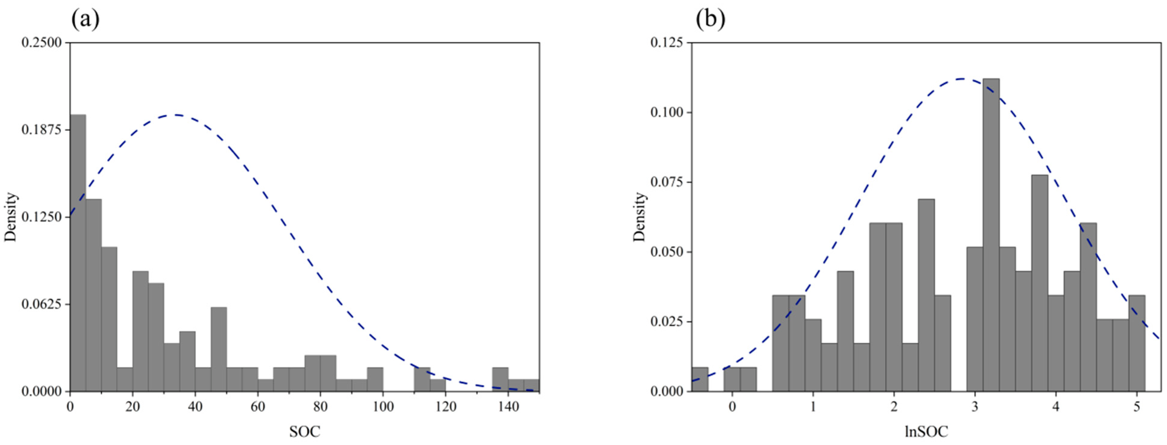
The SOC content of the samples ranges from 0.31 to 146.27 g/kg, with a mean of 28.33 g/kg and a standard deviation of 33.65 g/kg. The frequency distribution of SOC (Figure 3) exhibited a significantly positively skewed pattern, with a skewness of 1.71. Such an observation might reflect the complex natural conditions and high soil variabilities in the study area. Logarithmic transformation of SOC (termed hereafter lnSOC) is performed to make the data to be approximately symmetrically distributed. The result from the Kolmogorov–Smirnov (K–S) test indicated that the normality of the distribution of lnSOC (p = 0.012) has been greatly improved with respect to that of SOC (p = 0.000). The descriptive statistics of SOC and lnSOC are shown in Table 2.

3.2. Parameter Selection and Model Performance

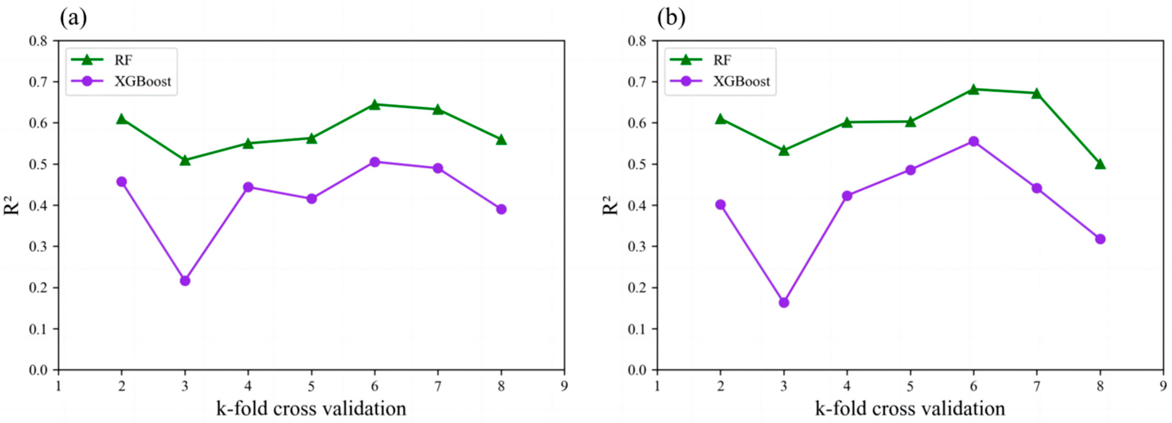
Figure 4 shows the results of model performance against the k-fold cross-validation for scenario A and B. The varying patterns of the model performance represented by R 2 for RF and XGBoost are similar, but RF consistently outperforms XGBoost. Both RF and XGBoost achieve the best performance when the number of folds is set to six, where the highest R 2 can reach 0.68 and 0.56 for RF and XGBoost, respectively.
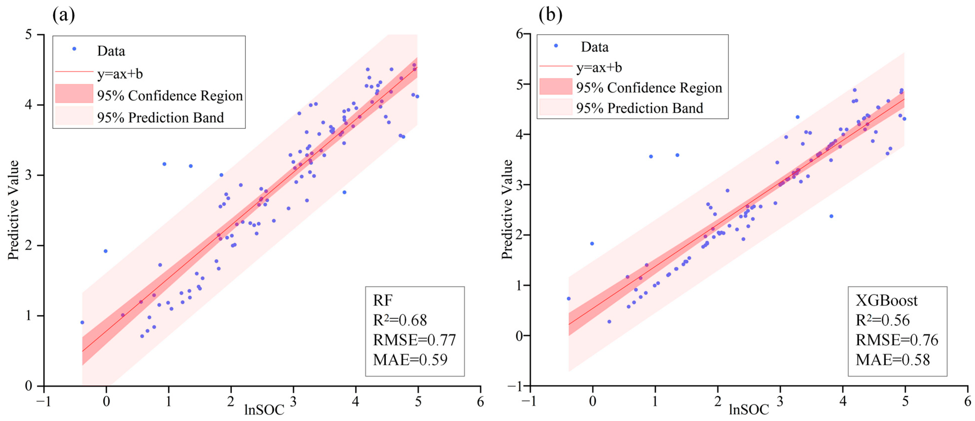
Figure 5 shows the detailed information of model performance for RF and XGBoost when six-fold cross validation was used. For both scenarios A and B, the model performance of RF is more satisfactory than XGBoost. For scenario A, the R2 of RF is 0.64, which is 27.58% higher than that of XGBoost. For scenario B, the R2 of RF is 0.68, which is 22.83% higher than that of XGBoost. However, the situation is slightly different in terms of RMSE and MAE. For scenario A, the RMSE of RF and XGBoost is the same, while the MAE of RF is slightly lower than that of XGBoost. For scenario B, both the RMSE and the MAE of XGBoost are a little lower than those of RF. As shown in Figure 6, a visual analysis of the predictions against the observed values also indicated that RF outperforms XGBoost. Such observation suggested that RF has better applicability for SOC prediction in areas with complex natural conditions and large regional variations.

3.3. SOC Distribution Predicted by RF

The spatial distribution of SOC content predicted by RF in scenario A and B is shown in Figure 7. In scenario A (Figure 7a), it can be found that the SOC contents range from 4.38 to 44.85 g/kg, with a mean of 23.22 g/kg. The SOC content is significantly higher in the southern area than in the northern area, and a clear boundary can be identified between them. Additionally, in the southwestern part, the SOC content is systematically higher than that in the northeastern part, which coincides well with the distribution pattern of elevation. In scenario B (Figure 7b), the range of SOC content predicted by RF is 3.86–47.68 g/kg. This data range is larger compared with the range for scenario A. This indicates that incorporation of phenological variables can provide more abundant information about SOC and can highlight the distribution characteristics. The spatial distribution patterns of the SOC content for scenario B are similar to that of the scenario A, but the local variation patterns in the northern area are clearly different for these scenarios. The spatial distribution patterns of the SOC content for scenario B are clearer, especially in the northeastern part of the study area. In addition, comparing Figure 2 and Figure 7b, the SOC content is much higher in the area with better vegetation growth, demonstrating the close connection between phenological variables and SOC.

3.4. Importance Ranking of Variables

The importance ranking of variables obtained by RF is shown in Figure 8. Among the variables evaluated, two climate variables, i.e., MAT and MAP, rank within the top three positions for both scenario A and B, where the two variables in total account for 34% and 24% of the variabilities, respectively. NDVI and DEM also play important roles in predicting SOC content. NDVI explains 20% and 11% of the variabilities for scenario A and B, respectively, and hence is the most important variable for SOC prediction in scenario A. This observation demonstrates that vegetation has a strong connection with SOC content. Among the topographic variables, DEM seems to be the most crucial one for SOC prediction, followed successively by slope, TWI, aspect and CA. For scenario B (Figure 8b), phenological variables explain in total 39% of the SOC variabilities, which is the highest proportion among the five types of environmental factors. After incorporation of the phenological variables, the importance of climate, topography, NDVI and land use decreased 10%, 15%, 9% and 4%, respectively, where the topographic variables were most affected by the phenological variables.

4. Discussion

4.1. Importance of Commonly Used Variables

As shown in Figure 8, it is obvious that climate is the dominant natural factor controlling the distribution of SOC content in this region. Ogle [72,73] found that climate can directly affect the sequestration and decomposition rate of SOC due to the variation of temperature and precipitation. Studies also show that MAP can help improve the vegetation productivity by increasing the atmospheric moisture and soil moisture, which further imposes positive effects on the SOC content [74]. MAT typically affects the concentration of SOC by controlling plant photosynthetic rate and microbial activity [75]. In particular, excessively high temperatures can harm SOC storage by destroying the activity of microorganisms and enzymes. The result (Figure 8) also indicates that NDVI is important in SOC prediction. It is well known that vegetation is the main source of soil carbon, and NDVI can well represent the degree of vegetation coverage of a region. Kaur [76] demonstrated that vegetation plays a crucial role in influencing SOC content by affecting litter accumulation and organic matter input from roots. This effect is particularly noticeable in surface soils. DEM also contributes much to the prediction of SOC content. Previous studies have suggested that high elevations have significant potential for storing SOC [34,39]. This may be why the alpine area, typically characterized by higher rainfall, lower temperature and less human interference, can provide suitable conditions for SOC storage. Specifically, DEM is usually associated with the vertical zonation of climate, which is characterized by a terrestrial landscape that changes dramatically with an increase in altitude [77,78]. Altitudinal zonation can result in rapid changes in air temperature and rainfall with increasing altitude, which can impact vegetation and hence the SOC accumulation [73]. In addition, population density usually decreases with the increase of altitude, so the influence of human activities (e.g., farming, logging and ranching) declines, which may also help maintain SOC content. Other topographical variables (i.e., slope, aspect, etc.) exhibit varying degrees of impact on the prediction of SOC content. For example, steep slopes, can accelerate the rate of soil erosion, resulting in negative effects on SOC accumulation in areas with relatively low vegetation coverage. Nevertheless, Sreenivas [18] found that the impact of topography on SOC is much lower than other environmental variables in his study area. A large proportion of his study region is characterized by either relatively flat and open terrain or simple topography, which, to some degree, explains the less important role of terrain factors in SOC prediction.

4.2. The Effect of Phenological Variables

The phenological variables are indicators of vegetation response to climate change, which can indirectly affect the dynamics of SOC by influencing the vegetation productivity [79]. Among the phenological variables, the difference between Greenup and Dormancy can represent the length of vegetation growing season. The longer the growing season, the more carbon will be produced in soil, hence contributing to SOC accumulation [80]. As can be seen in Figure 8, “2010_Greenup” is the most important among the phenological variables. A smaller Greenup value indicates an earlier starting time for the vegetation growth, and the length of the growing season will change accordingly, which will impose a positive effect on SOC accumulation [22]. The variable “2010_Peak” ranks as the second most influential phenological factor, likely because it represents the peak period of vigorous vegetation growth that can generate a substantial amount of carbon. In addition, soil fertility and its nutrient structure can conversely affect vegetation growth and development, which further affects the accumulation of SOC content. The above evidence can support the observation that the introduction of the phenological variables can help improve the accuracy of SOC prediction.
Note that the phenological variables were considered, by a trade-off of the model performance and computational complexity, for a time span of only four years in this study. Some studies [23,28] showed that historical phenology with 10 years and even longer may also exert an influence on SOC prediction. An improvement of the model performance can be expected by considering the phenological variables with a longer time range, which will be investigated in future studies.

4.3. Spatial Distribution of SOC Content

The spatial distribution of SOC content predicted by RF for scenario A and B are presented in Figure 7. The SOC content in the south, where the upper reaches of Heihe River Basin are located, is significantly higher than that in the north, which coincides with the pattern suggested by the sparse observations. The upper reaches of Heihe River Basin are characterized by higher altitudes, more abundant precipitation and lower temperature, providing more suitable conditions for SOC accumulation. Studies [81] have demonstrated that vegetation growth begins earlier with increasing altitude, resulting in a longer growth period that facilitates the SOC accumulation. In addition, the upper reaches of the Heihe River Basin are characterized by shrub and forest land use types, whereas the middle reaches are primarily composed of cultivated and barren land. Martín [82] found that the SOC content would typically increase when land use types changed from arable land to grassland or forest. This may be because the decrease of cultivated land areas and related agricultural activities (e.g., crop rotation, fertilization, and straw burning) can usually lead to the reduced influence on the soil, such that SOC can avoid being lost. In addition, the distribution pattern of SOC content, predicted by the RF model with the phenological variables being considered, is clearer than that from the scenario where the phenological variables were neglected, especially in the northern region. Such an observation might suggest that phenological variables can account for the SOC distribution patterns where the terrain is relatively flat and open. By contrast, the importance of phenological factors might be screened by the topographic factors in areas with large topographic relief. Previous studies [83] also suggested that the spatial distribution of SOC in this area was highly correlated with the topography and climate, which was consistent with the resulting patterns of SOC content in this study.
Note also that the range and the variability of the SOC content predicted by RF (Figure 7) have been narrowed down, compared with the original observations. Some scholars [67,84] ascribed this observation to the low accuracy of models, which were primarily influenced by the low density of sampling points. Nevertheless, the spatial distribution of the SOC content can still provide crucial information on the local variation patterns, which can further support the formulation of land management strategies.

4.4. Effect of Land Use Types on SOC Content Prediction

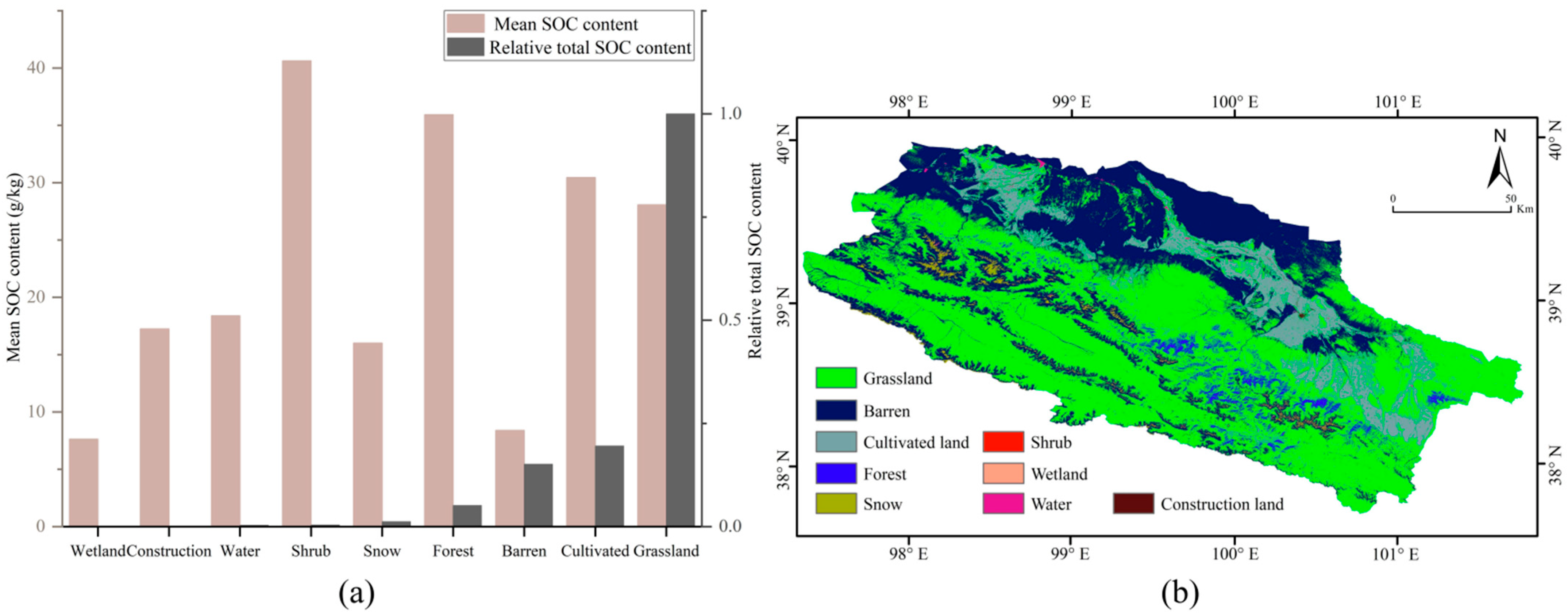
To investigate the effect of land use types on SOC content prediction, the mean SOC content and total SOC content of different land use types were further calculated (Figure 9). Grassland, cultivated land and barren land have higher total SOC content, which is largely due to their relatively higher area proportions. For example, the grassland shows the greatest potential for SOC storage considering that it accounts for about 57% of the total area. In contrast, the area occupied by shrub is minimal, such that the total SOC content within it is very low. However, the mean SOC content in the shrub is the highest, which may be because most shrub is distributed in the area with high altitude, where it is characterized by wet, low temperature and low population density, resulting in a suitable condition for SOC storage. The forest land has the second highest mean SOC content. One important reason is that forest has abundant leaves and microorganisms, which can provide plentiful sources for SOC accumulation. In brief, land use types that are related with natural conditions, population density, soil construction and soil nutrient, etc., can impose significant effect on SOC distribution.

5. Conclusions

This study used machine learning methods, based on the commonly used environmental variables (i.e., topography, climate, vegetation index and land use types), combined with the phenological variables extracted from MODIS data product (MCD12Q2), to predict the SOC content in the middle and upper reaches of the Heihe River Basin. The following conclusions can be drawn thereby:
(1)
Adding phenological variables can help further improve the model performance for SOC prediction. When accounting for phenological variables, RF and XGBoost models exhibit R2 values of 0.68 and 0.56, respectively, which represents a 6% and 10% increase compared to the scenario where phenological variables are neglected in the case study.
(2)
Both RF and XGBoost can effectively predict the SOC content, but RF can consistently achieve better performance than XGBoost in the study area for different cross-validation experiments.
(3)
In the middle and upper reaches of the Heihe River Basin, the spatial distribution of SOC content showed a discernible trend that decreases from the south to the north. The factors of MAP, MAT, NDVI and DEM showed the greatest impact on the prediction of SOC content.
This study confirms that phenological variables are effective predictors for modeling SOC content. A more accurate mapping of SOC content can be obtained by using the combination of the phenological variables and the commonly used environmental variables in the predictive modeling, which could provide valuable information for soil management and environment protection in the future.
Future study should focus on examining the heterogeneous effect of the phenological variables on SOC prediction in the study area, and their applications for SOC prediction in areas characterized by other types of topographic and climatic conditions.

Author Contributions

Conceptualization, J.W.; methodology, X.L. and J.W.; software, X.L.; investigation, X.L. and J.W.; resources, X.L.; visualization, X.L.; writing—original draft preparation, X.L.; writing—review and editing, X.L., J.W. and X.S.; supervision, J.W. and X.S. All authors have read and agreed to the published version of the manuscript.

Funding

The National Natural Science Foundation of China (No. 42002295).

Data Availability Statement

The data used in this study are publicly available online in the Resource and Environment Science and Data Center at https://www.resdc.cn/ (accessed on 21 March 2022), and in the USGS at https://www.usgs.gov/ (accessed on 8 July 2022).

Acknowledgments

The first author thanks Y.H. Shi for help in processing the data.

Conflicts of Interest

The authors declare no conflict of interest.

References

  1. Wu, H.; Guo, Z.; Peng, C. Distribution and storage of soil organic carbon in China. Glob. Biogeochem. Cycles 2003, 17, 1048. [Google Scholar] [CrossRef] [Green Version]
  2. Stockmann, U.; Padarian, J.; McBratney, A.; Minasny, B.; de Brogniez, D.; Montanarella, L.; Field, D.J. Global soil organic carbon assessment. Glob. Food Secur. 2015, 6, 9–16. [Google Scholar] [CrossRef]
  3. Xu, L.; Zhang, Z.Q.; Sun, Y.Q.; Mao, P. Estimation of soil organic carbon storage in Mountains based on Three-dimensional Curved Surface: A case study of Lushan. Soil Bull. 2019, 50, 1101–1107. [Google Scholar]
  4. Ramifehiarivo, N.; Brossard, M.; Grinand, C.; Andriamananjara, A.; Razafimbelo, T.; Rasolohery, A.; Razafimahatratra, H.; Seyler, F.; Ranaivoson, N.; Rabenarivo, M.; et al. Mapping soil organic carbon on a national scale: Towards an improved and updated map of Madagascar. Geoderma Reg. 2017, 9, 29–38. [Google Scholar] [CrossRef]
  5. Yang, X.-M.; Wander, M.M. Tillage effects on soil organic carbon distribution and storage in a silt loam soil in Illinois. Soil Tillage Res. 1999, 52, 1–9. [Google Scholar] [CrossRef]
  6. Wang, S.Q.; Liu, J.Y.; Yu, G.R. Error analysis of soil organic carbon storage estimation in China. Chin. J. Appl. Ecol. 2003, 5, 797–802. [Google Scholar]
  7. Li, T.T.; Ji, H.B.; Sun, Y.Y.; Luo, J.M.; Jiang, Y.B.; Wang, L.X. Research progress on soil organic carbon storage and its in-fluencing factors. J. Cap. Norm. Univ. 2007, 1, 93–97. [Google Scholar]
  8. Jin, F.; Yang, H.; Zhao, Q.G. Research progress of soil organic carbon storage and its influencing factors. Soil 2007, 2000, 12–18. [Google Scholar]
  9. Elbasiouny, H.; Abowaly, M.; Abu_Alkheir, A.; Gad, A. Spatial variation of soil carbon and nitrogen pools by using ordinary Kriging method in an area of north Nile Delta, Egypt. Catena 2014, 113, 70–78. [Google Scholar] [CrossRef]
  10. Zhu, A.X.; Yang, L.; Fan, N.Q.; Zeng, C.Y.; Zhang, G.L. Review and Prospect of digital soil mapping research. Prog. Geogr. 2018, 37, 66–78. [Google Scholar]
  11. McBratney, A.B.; Santos, M.M.; Minasny, B. On digital soil mapping. Geoderma 2003, 117, 3–52. [Google Scholar] [CrossRef]
  12. Pendleton, R.L.; Jenny, H. Factors of Soil Formation: A System of Quantitative Pedology. Geogr. Rev. 1945, 35, 336. [Google Scholar] [CrossRef]
  13. Song, M.; Yang, L.; Zhu, A.X.; Qin, C.Z. Rotation mode application in farming area of soil organic matter that mapping. J. Soil Bull. 2017, 48, 778–785. [Google Scholar]
  14. Zhou, T.; Shi, P.J.; Wang, S.Q. Impacts of climate change and human activities on soil organic carbon storage in China. Acta Geogr. Sin. 2003, 58, 727–734. [Google Scholar]
  15. Wei, Y.C.; Lu, X.L.; Zhu, C.D.; Zhang, X.X.; Pan, J.J. High-resolution Digital Mapping of Soil Organic Carbon at Small Wa-tershed Scale Using Landform Element Classification and Assisted Remote Sensing Information. Acta Pedol. Sin. 2022, 60, 1–15. [Google Scholar]
  16. Lamichhane, S.; Kumar, L.; Wilson, B. Digital soil mapping algorithms and covariates for soil organic carbon mapping and their implications: A review. Geoderma 2019, 352, 395–413. [Google Scholar] [CrossRef]
  17. Adeniyi, O.D.; Brenning, A.; Bernini, A.; Brenna, S.; Maerker, M. Digital Mapping of Soil Properties Using Ensemble Machine Learning Approaches in an Agricultural Lowland Area of Lombardy, Italy. Land 2023, 12, 494. [Google Scholar] [CrossRef]
  18. Sreenivas, K.; Dadhwal, V.; Kumar, S.; Harsha, G.S.; Mitran, T.; Sujatha, G.; Suresh, G.J.R.; Fyzee, M.; Ravisankar, T. Digital mapping of soil organic and inorganic carbon status in India. Geoderma 2016, 269, 160–173. [Google Scholar] [CrossRef]
  19. Angelopoulou, T.; Tziolas, N.; Balafoutis, A.; Zalidis, G.; Bochtis, D. Remote sensing techniques for soil organic carbon es-timation: A review. Remote Sens. 2019, 11, 676. [Google Scholar] [CrossRef] [Green Version]
  20. Zhang, Y.; Guo, L.; Chen, Y.; Shi, T.; Luo, M.; Ju, Q.; Zhang, H.; Wang, S. Prediction of Soil Organic Carbon based on Landsat 8 Monthly NDVI Data for the Jianghan Plain in Hubei Province, China. Remote Sens. 2019, 11, 1683. [Google Scholar] [CrossRef] [Green Version]
  21. Yang, L.; He, X.; Shen, F.; Zhou, C.; Zhu, A.-X.; Gao, B.; Chen, Z.; Li, M. Improving prediction of soil organic carbon content in croplands using phenological parameters extracted from NDVI time series data. Soil Tillage Res. 2019, 196, 104465. [Google Scholar] [CrossRef]
  22. Zhang, L.; Cai, Y.; Huang, H.; Li, A.; Yang, L.; Zhou, C. A CNN-LSTM Model for Soil Organic Carbon Content Prediction with Long Time Series of MODIS-Based Phenological Variables. Remote Sens. 2022, 14, 4441. [Google Scholar] [CrossRef]
  23. Richardson, A.D.; Hollinger, D.Y.; Dail, D.B.; Lee, J.T.; Munger, J.W.; O’Keefe, J. Influence of spring phenology on seasonal and annual carbon balance in two contrasting New England forests. Tree Physiol. 2009, 29, 321–331. [Google Scholar] [CrossRef] [PubMed]
  24. Ji, X.F.; Gong, Y.; Zheng, X.; Jiang, J.; Lu, J.B.; Liu, S.L.; Wang, D.; Fang, W.L.; He, X.K. Carbon Exchange and phenological characteristics of forest ecosystem in Fengyang Mountain. J. Earth Environ. 2020, 11, 376–389. [Google Scholar]
  25. Wu, Z.H.; Wang, X.Y. Changes in Phenology of Typical Grassland in China Based on NDVI Data and Its Effect on Productivity. Remote Sens. Technol. Appl. 2023, 1–11. Available online: http://kns.cnki.net/kcms/detail/62.1099.TP.20230227.1720.002.html (accessed on 14 March 2023).
  26. Wei, X.S.; Gao, Y.L.; Fan, Y.Q.; Lin, L.; Mao, J.; Zhang, D.H.; Li, X.H.; Liu, X.Y.; Xu, M.Z.; Tian, Y.; et al. Responses of net primary productivity to phenological changes in Beijing. Agric. Eng. 2022, 38, 167–175. [Google Scholar]
  27. Kariyeva, J.; Van Leeuwen, W.J.D. Environmental Drivers of NDVI-Based Vegetation Phenology in Central Asia. Remote Sens. 2011, 3, 203–246. [Google Scholar] [CrossRef] [Green Version]
  28. Yang, L.; Cai, Y.; Zhang, L.; Guo, M.; Li, A.; Zhou, C. A deep learning method to predict soil organic carbon content at a regional scale using satellite-based phenology variables. Int. J. Appl. Earth Obs. Geoinf. 2021, 102, 102428. [Google Scholar] [CrossRef]
  29. He, X.; Yang, L.; Li, A.; Zhang, L.; Shen, F.; Cai, Y.; Zhou, C. Soil organic carbon prediction using phenological parameters and remote sensing variables generated from Sentinel-2 images. Catena 2021, 205, 105442. [Google Scholar] [CrossRef]
  30. Xia, C.F.; Li, J.; Liu, Q.H. Review of advances in vegetation phenology monitoring by remote sensing. J. Remote Sens. 2013, 17, 1–16. [Google Scholar]
  31. Friedl, M.; Gray, J.; Sulla-Menashe, D. MCD12Q2 MODIS/Terra+Aqua Land Cover Dynamics Yearly L3 Global 500m SIN Grid V006. NASA EOSDIS Land Processes DAAC 2019. Available online: https://lpdaac.usgs.gov/documents/1310/mcd12q2_v6_user_guide.pdf (accessed on 14 March 2023).
  32. John, K.; Isong, I.A.; Kebonye, N.M.; Ayito, E.O.; Agyeman, P.C.; Afu, S.M. Using Machine Learning Algorithms to Estimate Soil Organic Carbon Variability with Environmental Variables and Soil Nutrient Indicators in an Alluvial Soil. Land 2020, 9, 487. [Google Scholar] [CrossRef]
  33. Odebiri, O.; Odindi, J.; Mutanga, O. Basic and deep learning models in remote sensing of soil organic carbon estimation: A brief review. Int. J. Appl. Earth Obs. Geoinf. 2021, 102, 102389. [Google Scholar] [CrossRef]
  34. Song, X.D.; Brus, D.J.; Liu, F.; Li, D.C.; Zhao, Y.G.; Yang, J.L.; Zhang, G.L. Mapping soil organic carbon content by geo-graphically weighted regression: A case study in the Heihe River Basin, China. Geoderma 2016, 261, 11–22. [Google Scholar] [CrossRef]
  35. Gomes, L.C.; Faria, R.M.; de Souza, E.; Veloso, G.V.; Schaefer, C.E.G.; Filho, E.I.F. Modelling and mapping soil organic carbon stocks in Brazil. Geoderma 2019, 340, 337–350. [Google Scholar] [CrossRef]
  36. Qi, Y.B.; Wang, Y.Y.; Chen, Y.; Liu, J.J.; Zhang, L.L. Soil Organic Matter Prediction Based on Remote Sensing Data and Random Forest Model in Shaanxi Province. J. Nat. Resour. 2017, 32, 1074–1086. [Google Scholar]
  37. Szatmári, G.; Pásztor, L.; Heuvelink, G.B. Estimating soil organic carbon stock change at multiple scales using machine learning and multivariate geostatistics. Geoderma 2021, 403, 115356. [Google Scholar] [CrossRef]
  38. Guo, L.; Fu, P.; Shi, T.; Chen, Y.; Zeng, C.; Zhang, H.; Wang, S. Exploring influence factors in mapping soil organic carbon on low-relief agricultural lands using time series of remote sensing data. Soil Tillage Res. 2021, 210, 104982. [Google Scholar] [CrossRef]
  39. Yang, R.-M.; Zhang, G.-L.; Liu, F.; Lu, Y.-Y.; Yang, F.; Yang, F.; Yang, M.; Zhao, Y.-G.; Li, D.-C. Comparison of boosted regression tree and random forest models for mapping topsoil organic carbon concentration in an alpine ecosystem. Ecol. Indic. 2015, 60, 870–878. [Google Scholar] [CrossRef]
  40. Lai, Y.Q.; Sun, X.L.; Wang, H.L. Mapping of Soil Organic Carbon Using Neural Network and Its Mixed Model with Geosta-tistics in a Small Area of Typical Hilly Region. Chin. J. Soil Sci. 2020, 51, 1313–1322. [Google Scholar]
  41. Liu, W.; Zhu, M.; Li, Y.; Zhang, J.; Yang, L.; Zhang, C. Assessing Soil Organic Carbon Stock Dynamics under Future Climate Change Scenarios in the Middle Qilian Mountains. Forests 2021, 12, 1698. [Google Scholar] [CrossRef]
  42. Ding, J.Z.; Li, F.; Yang, G.B.; Chen, L.Y.; Zhang, B.B.; Liu, L.; Fang, K.; Qin, S.Q.; Chen, Y.L.; Peng, Y.F.; et al. The per-mafrost carbon inventory on the Tibetan Plateau: A new evaluation using deep sediment cores. Glob. Chang. Biol. 2016, 22, 2688–2701. [Google Scholar] [CrossRef] [Green Version]
  43. Li, G.; Ma, D.; Zhao, C.; Li, H. The Effect of the Comprehensive Reform of Agricultural Water Prices on Farmers’ Planting Structure in the Oasis–Desert Transition Zone—A Case Study of the Heihe River Basin. Int. J. Environ. Res. Public Health 2023, 20, 4915. [Google Scholar] [CrossRef] [PubMed]
  44. Song, W.; Zhang, Y. Expansion of agricultural oasis in the Heihe River Basin of China: Patterns, reasons and policy implications. Phys. Chem. Earth Parts A/B/C 2015, 89, 46–55. [Google Scholar] [CrossRef]
  45. Yi, Z.; Wei, X.J.; Song, X.Y. Research on the precipitation characteristics in the upper and middle reaches of Heihe River during 1990–2012. China Rural. Water Hydropower 2019, 3, 92–96. [Google Scholar]
  46. Lu, Z.; Han, M.L.; Lu, H.; Peng, X.T.; Men, G.S.; Liu, J.; Yang, X.F. Estimation soil moisture in the middle and upper reaches of Heihe River based on AMSR2 Multi-brightness temperature. Remote Sens. Technol. Appl. 2020, 35, 33–47. [Google Scholar]
  47. Li, X.; Ma, M.G.; Wang, J.; Liu, Q.; Che, T.; Hu, Z.Y.; Xiao, Q.; Liu, Q.H.; Su, P.X.; Chu, R.Z.; et al. Simultaneous remote sensing and ground-based experiment in the Heihe river basin Scientific objective and experiment design. Adv. Earth Sci. 2008, 9, 897–914. [Google Scholar]
  48. Li, Y.L.; Yan, D.H.; Pei, Y.S.; Qin, D.Y. Dynamic of variation landscape in Heihe river basin. J. Hohai Univ. 2005, 1, 6–10. [Google Scholar]
  49. Song, X.-D.; Wu, H.-Y.; Ju, B.; Liu, F.; Yang, F.; Li, D.-C.; Zhao, Y.-G.; Yang, J.-L.; Zhang, G.-L. Pedoclimatic zone-based three-dimensional soil organic carbon mapping in China. Geoderma 2019, 363, 114145. [Google Scholar] [CrossRef]
  50. Zhang, G.L.; Gong, Z.T. Methods for Laboratory Analysis of Soil Survey; Science Press: Beijing, China, 2012. [Google Scholar]
  51. Chen, D.; Chang, N.; Xiao, J.; Zhou, Q.; Wu, W. Mapping dynamics of soil organic matter in croplands with MODIS data and machine learning algorithms. Sci. Total Environ. 2019, 669, 844–855. [Google Scholar] [CrossRef]
  52. Wang, S.; Xu, L.; Zhuang, Q.; He, N. Investigating the spatio-temporal variability of soil organic carbon stocks in different ecosystems of China. Sci. Total Environ. 2020, 758, 143644. [Google Scholar] [CrossRef] [PubMed]
  53. Emadi, M.; Taghizadeh-Mehrjardi, R.; Cherati, A.; Danesh, M.; Mosavi, A.; Scholten, T. Predicting and Mapping of Soil Organic Carbon Using Machine Learning Algorithms in Northern Iran. Remote Sens. 2020, 12, 2234. [Google Scholar] [CrossRef]
  54. Conrad, O.; Bechtel, B.; Bock, M.; Dietrich, H.; Fischer, E.; Gerlitz, L.; Wehberg, J.; Wichmann, V.; Böhner, J. System for Automated Geoscientific Analyses (SAGA) v. 2.1.4. Geosci. Model Dev. 2015, 8, 1991–2007. [Google Scholar] [CrossRef] [Green Version]
  55. Zhou, T.; Geng, Y.; Chen, J.; Liu, M.; Haase, D.; Lausch, A. Mapping soil organic carbon content using multi-source remote sensing variables in the Heihe River Basin in China. Ecol. Indic. 2020, 114, 106288. [Google Scholar] [CrossRef]
  56. Resource and Environment Science and Data Center. Available online: https://www.resdc.cn/ (accessed on 21 March 2022).
  57. Yang, J.; Huang, X. The 30 m annual land cover dataset and its dynamics in China from 1990 to 2019. Earth Syst. Sci. Data 2021, 13, 3907–3925. [Google Scholar] [CrossRef]
  58. United States Geological Survey. Available online: https://www.usgs.gov/ (accessed on 9 July 2022).
  59. Wu, C.W.; Liang, J.H.; Wang, W.; Li, C.S. Random forest algorithm based on recursive feature elimination methods. Stat. Decis. Mak. 2017, 21, 60–63. [Google Scholar]
  60. Stevens, A.; Nocita, M.; Toth, G.; Montanarella, L.; van Wesemael, B. Prediction of Soil Organic Carbon at the European Scale by Visible and Near InfraRed Reflectance Spectroscopy. PLoS ONE 2013, 8, e66409. [Google Scholar] [CrossRef]
  61. Xiao, Y.; Xue, J.; Zhang, X.; Wang, N.; Hong, Y.; Jiang, Y.; Zhou, Y.; Teng, H.; Hu, B.; Lugato, E.; et al. Improving pedotransfer functions for predicting soil mineral associated organic carbon by ensemble machine learning. Geoderma 2022, 428, 116208. [Google Scholar] [CrossRef]
  62. Breiman, L. Random forests. Mach. Learn. 2001, 45, 5–32. [Google Scholar] [CrossRef] [Green Version]
  63. Lv, H.Y.; Feng, Q. A Review of random forest algorithm. J. Hebei Acad. Sci. 2019, 36, 37–41. [Google Scholar]
  64. Yu, X.Y.; Zhao, G.X.; Chang, C.Y.; Yuan, X.J.; Wang, Z.R. Random forest classifier in remote sensing information extraction: A review of application and feature development. Remote Sens. Inf. 2019, 34, 8–14. [Google Scholar]
  65. Zhang, H.; Wu, P.; Yin, A.; Yang, X.; Zhang, M.; Gao, C. Prediction of soil organic carbon in an intensively managed rec-lamation zone of eastern China: A comparison of multiple linear regressions and the random forest model. Sci. Total Environ. 2017, 592, 704–713. [Google Scholar] [CrossRef] [PubMed]
  66. Wang, B.; Gray, J.M.; Waters, C.M.; Anwar, M.R.; Orgill, S.E.; Cowie, A.L.; Feng, P.; Liu, D.L. Modelling and mapping soil organic carbon stocks under future climate change in south-eastern Australia. Geoderma 2021, 405, 115442. [Google Scholar] [CrossRef]
  67. Were, K.; Bui, D.T.; Dick, Ø.B.; Singh, B.R. A comparative assessment of support vector regression, artificial neural networks, and random forests for predicting and mapping soil organic carbon stocks across an Afromontane landscape. Ecol. Dicators 2015, 52, 394–403. [Google Scholar] [CrossRef]
  68. Chen, T.; Guestrin, C. XGBoost: A Scalable Tree Boosting System. In Proceedings of the 22nd ACM SIGKDD International Conference on Knowledge Discovery and Data Mining, San Francisco, CA, USA, 13–17 August 2016; pp. 785–794. [Google Scholar]
  69. Liang, Z.; Chen, S.; Yang, Y.; Zhou, Y.; Shi, Z. High-resolution three-dimensional mapping of soil organic carbon in China: Effects of SoilGrids products on national modeling. Sci. Total. Environ. 2019, 685, 480–489. [Google Scholar] [CrossRef]
  70. Wang, H.; Zhang, X.; Wu, W.; Liu, H. Prediction of Soil Organic Carbon under Different Land Use Types Using Sentinel-1/-2 Data in a Small Watershed. Remote Sens. 2021, 13, 1229. [Google Scholar] [CrossRef]
  71. Xie, B.; Ding, J.; Ge, X.; Li, X.; Han, L.; Wang, Z. Estimation of Soil Organic Carbon Content in the Ebinur Lake Wetland, Xinjiang, China, Based on Multisource Remote Sensing Data and Ensemble Learning Algorithms. Sensors 2022, 22, 2685. [Google Scholar] [CrossRef]
  72. Ogle, S.M.; Breidt, F.J.; Paustian, K. Agricultural management impacts on soil organic carbon storage under moist and dry climatic conditions of temperate and tropical regions. Biogeochemistry 2005, 72, 87–121. [Google Scholar] [CrossRef]
  73. Hu, P.-L.; Liu, S.-J.; Ye, Y.-Y.; Zhang, W.; Wang, K.-L.; Su, Y.-R. Effects of environmental factors on soil organic carbon under natural or managed vegetation restoration. Land Degrad. Dev. 2018, 29, 387–397. [Google Scholar] [CrossRef]
  74. Jobbágy, E.G.; Jackson, R.B. The vertical distribution of soil organic carbon and its relation to climate and vegetation. Ecol. Appl. 2000, 10, 423–436. [Google Scholar] [CrossRef]
  75. Ding, J.M.; Wang, W.Z.; Mi, W.B.; Hou, K.Y.; Zhang, X.W.; Zhao, Y.N.; Wen, Q. Spatial chracteristics of soil organic carbon in grassland of Ningxia and its influence factors. Acta Ecol. Sin. 2023, 43, 1913–1922. [Google Scholar]
  76. Kaur, B.; Gupta, S.; Singh, G. Soil carbon, microbial activity and nitrogen availability in agroforestry systems on moderately alkaline soils in northern India. Appl. Soil Ecol. 2000, 15, 283–294. [Google Scholar] [CrossRef]
  77. Zhou, T.; Geng, Y.; Chen, J.; Pan, J.; Haase, D.; Lausch, A. High-resolution digital mapping of soil organic carbon and soil total nitrogen using DEM derivatives, Sentinel-1 and Sentinel-2 data based on machine learning algorithms. Sci. Total Environ. 2020, 729, 138244. [Google Scholar] [CrossRef]
  78. Kheir, R.B.; Greve, M.H.; Bøcher, P.K.; Greve, M.B.; Larsen, R.; McCloy, K. Predictive mapping of soil organic carbon in wet cultivated lands using classification-tree based models: The case study of Denmark. J. Environ. Manag. 2010, 91, 1150–1160. [Google Scholar] [CrossRef] [PubMed]
  79. Wang, Y.; Yang, X.; Hao, L.N. Phenology of vegetation and its response to climate change in the west Sichuan plateau. J. Yangtze River Sci. Res. Inst. 2022, 1–10. Available online: http://kns.cnki.net/kcms/detail/42.1171.tv.20220715.1632.002.html (accessed on 11 December 2022).
  80. Li, X.; Du, H.; Zhou, G.; Mao, F.; Zhang, M.; Han, N.; Fan, W.; Liu, H.; Huang, Z.; He, S.; et al. Phenology estimation of subtropical bamboo forests based on assimilated MODIS LAI time series data. ISPRS J. Photogramm. Remote Sens. 2021, 173, 262–277. [Google Scholar] [CrossRef]
  81. Wang, Z.; Cao, S.; Cao, G.; Lan, Y. Effects of vegetation phenology on vegetation productivity in the Qinghai Lake Basin of the Northeastern Qinghai–Tibet Plateau. Arab. J. Geosci. 2021, 14, 1030. [Google Scholar] [CrossRef]
  82. Martín, J.R.; Álvaro-Fuentes, J.; Gonzalo, J.; Gil, C.; Ramos-Miras, J.; Corbí, J.G.; Boluda, R. Assessment of the soil organic carbon stock in Spain. Geoderma 2016, 264, 117–125. [Google Scholar] [CrossRef] [Green Version]
  83. Song, X.; Liu, F.; Zhang, G.; Li, D.; Zhao, Y.; Yang, J. Mapping Soil Organic Carbon Using Local Terrain Attributes: A Comparison of Different Polynomial Models. Pedosphere 2017, 27, 681–693. [Google Scholar] [CrossRef]
  84. Grimm, R.; Behrens, T.; Märker, M.; Elsenbeer, H. Soil organic carbon concentrations and stocks on Barro Colorado Is-land—Digital soil mapping using Random Forests analysis. Geoderma 2008, 146, 102–113. [Google Scholar] [CrossRef]
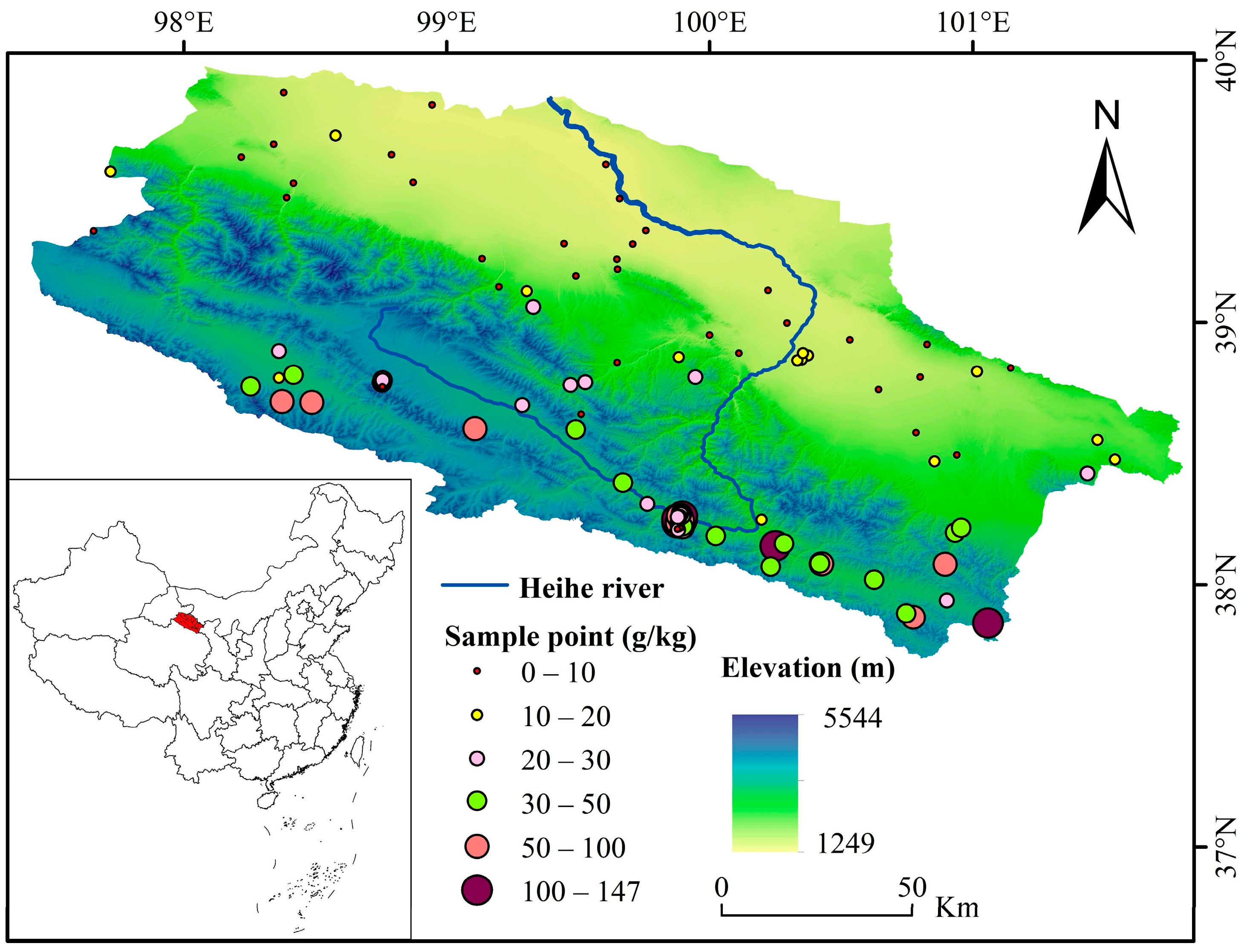
Figure 1. Location of study area and distribution of sample points.
Remotesensing 15 01847 g001
Figure 2. The spatial distribution of phenological variables Greenup (a) and Dormancy (b) in 2010. Note that values of the phenological variables represent accumulated days since 1 January 1970.
Remotesensing 15 01847 g002
Figure 3. Frequency distribution of SOC (a) and lnSOC (b).
Remotesensing 15 01847 g003
Figure 4. Model accuracy under k-fold cross validation with commonly used variables (a) and commonly used variables and phenological variables (b).
Remotesensing 15 01847 g004
Figure 5. The histogram of model accuracy of R 2 (a), RMSE (b), and MAE (c), when different environmental variables were used.
Remotesensing 15 01847 g005
Figure 6. Model fitting result by RF (a) and XGBoost (b) when phenological variables and normal variables were used.
Remotesensing 15 01847 g006
Figure 7. The spatial distribution of SOC content predicted by RF using commonly used variables (a) and commonly-used variables and phenological variables (b).
Remotesensing 15 01847 g007
Figure 8. Importance ranking of environmental variables by RF using commonly used variables (a) and commonly used variables and phenological variables (b).
Remotesensing 15 01847 g008
Figure 9. The mean SOC content and relative total SOC content of different land use types (a) and the spatial distribution of different land use types (b).
Remotesensing 15 01847 g009
Table 1. Information of environmental variables in the study area.
Factor CategoryVariablesResolutionTime Period
TopographyElevation
Aspect
Slope
Catchment Area (CA)
Topographic Wetness Index (TWI)
90 m-
ClimateMean annual temperature (MAT)
Mean annual precipitation (MAP)
1000 m2010–2019
Vegetation
index
Normalized Difference Vegetation Index (NDVI)1000 m2010–2019
Land useLand use types30 m-
Phenological variablesNumCycle
Greenup
MidGreenup
Peak
Maturity
Senescence
MidGreendown
Dormancy
EVI_Minimum
EVI_Amplitude
EVI_Area
500 m2010–2013
Table 2. Descriptive statistics of the original and logarithmic SOC observations.
Minimum
(g/kg)
Maximum
(g/kg)
Mean
(g/kg)
Standard Deviation (g/kg)Coefficient of Variation (%)Kurtosis
(%)
Skewness
(%)
SOC0.31146.2728.3333.651.192.481.71
lnSOC–1.174.982.591.330.51–0.69–0.17
Disclaimer/Publisher’s Note: The statements, opinions and data contained in all publications are solely those of the individual author(s) and contributor(s) and not of MDPI and/or the editor(s). MDPI and/or the editor(s) disclaim responsibility for any injury to people or property resulting from any ideas, methods, instructions or products referred to in the content.