Investigating the Backscatter of Marine Plastic Litter Using a C- and X-Band Ground Radar, during a Measurement Campaign in Deltares

Abstract

In recent years, marine plastic pollution has seen increased coverage in the public interest and research due to a greater understanding of the scale and impact of plastic pollution within the marine environment. Considering the hazard that plastic waste poses on the environment, marine life, and on humans, remote-sensing techniques could provide timely information on their detection and dynamics. The remote sensing of marine plastic is a relatively new field and research into the capabilities of radar for detecting and monitoring marine plastic pollution is generally limited, with several interactions and mechanisms being largely unknown. Here, we exploit the use of a C- and X-band radar to understand the capabilities of monitoring marine plastics. Our results show that backscattering differences in the C- and X-band between the reference water (called here as “clean”) and the test water filled with plastic can be detected in some conditions (based on statistical analysis). Overall, the results indicate that the X-band frequency performs significantly better than the C-band frequency, with X-band detecting significant differences in backscattering in 48/68 test cases compared with C-band detecting differences in 20/67 test cases. We also find that the difference in backscattering is dependent on the size and shape of the plastic object, as well as the wave conditions which the plastic is moving on. This study provides new insights on the radar capabilities for detecting marine plastic litter and new information which can be used in the planning of future missions and studies on the remote sensing of marine plastic pollution.

1. Introduction

Accumulations of plastic pollution are not well mapped globally [1]. There are an estimated 4.8–12.7 million metric tons of plastic that enter the ocean from land annually [2]. The presence of plastic in marine environments is of great concern, with at least 690 species worldwide being negatively affected by the presence of marine plastic pollution [3]. Animal species are both at risk of ingestion and entanglement with plastic pollution [4]. However, it is not only the marine species that are at risk from marine plastic pollution; there are multiple documented human health issues that are associated with plastics, including food safety and security [5], and health issues stemming from toxic by-products of plastics, such as cancer, respiratory disease, cardiovascular disease, and more [6]. Although plastics’ transportation within the ocean is beginning to gain some understanding, some models can differ by more than a factor of 100 [7]. Measurements of marine plastics have traditionally been performed in situ; however, complications can arise from budget, spatial, and accessibility issues.

There are an estimated 21,000 [8]–79,000 [9] tonnes of floating plastic inside the Great Pacific Garbage Patch alone, with over three-quarters of the garbage patch carrying debris that is larger than 5 cm [9]. Due to the known presence of surface plastics, remote sensing has been explored as a means of monitoring plastic pollution due to its effective history of being used for observing other ocean surface processes and phenomena [10]. At present, most research on the detection of plastic pollution has been undertaken with the use of spectral imaging. This includes work in visible [11], short-wave infrared [12], and near-infrared [13] parts of the electromagnetic spectrum. These optical studies have employed in situ, unmanned aerial vehicle (UAV) and satellite imagery (primarily with Sentinel-2). Reviews of the current literature have shown that the remote sensing of marine plastics can be improved through the use of different sensing technologies and methods to complement each other [14].

SAR is an active microwave imaging method capable of providing high-resolution monitoring of day-and-night imaging in nearly all weather conditions. SAR datasets have been used to measure physical properties of the Earth’s surface, such as glaciers, vegetation properties, topographies, and natural hazards, but are also extensively used in the monitoring of ocean environments [15,16]. The use of SAR has previously been used to detect biogenic films [17] and oil slicks [18], as well as targets such as derelict fishing gear and larger items [1]. However, the interactions of the marine debris with the background ocean can make exploitation with SAR challenging [1]. The use of SAR for monitoring small marine debris with SAR is largely understudied and not well understood. While there is some very recent research into radar’s capabilities for detecting and monitoring marine plastic debris [1,11,14,19,20], the way that backscatter interacts with differing plastic items is largely unknown. The use of satellite bands is also less known. The lack of research is even more evident when we consider the backscattering of small plastic debris in water. Sensor sensitivity, configuration, and optimisation need to be considered in the future to fully understand SAR’s capabilities.

This paper describes the theory and capabilities of radars operating on C- and X- band in observing floating plastic pollution in differing conditions through a series of measurement campaigns conducted in a lab setting. In this work, we address the following research questions:

• Does marine plastic pollution produce a change in backscattering in radar imagery at C- and X-band wavelengths when compared to the same conditions without plastic?
• What are the conditions that make this change statistically significant and what are the minimum quantities that we can observe?

The novelty of this study resides in the experiments carried out and the findings coming from the statistical analysis of those datasets. We show that radar backscatter differs between the reference and test conditions in multiple lab settings (wave conditions, plastic items, plastic concentrations) and that plastic pollution is potentially detectable in both C-band and X-band wavelengths, provided we have a reliable reference backscattering for the clean conditions. We also show the detection thresholds for specific plastic item concentrations in differing wave conditions.

The overall aim of this research is to find out if Synthetic Aperture Radar satellite data could be used to discriminate areas of large accumulations of floating plastics. There are already evidences of this, such as in Simpson et al., 2022 [21], and these experiments try to shed a light on the understanding of backscattering from plastic in water, using different plastic items, concentrations, and conditions.

2. Materials and Methods

2.1. Deltares Experiment: Lab Conditions and Ocean Wave Spectra

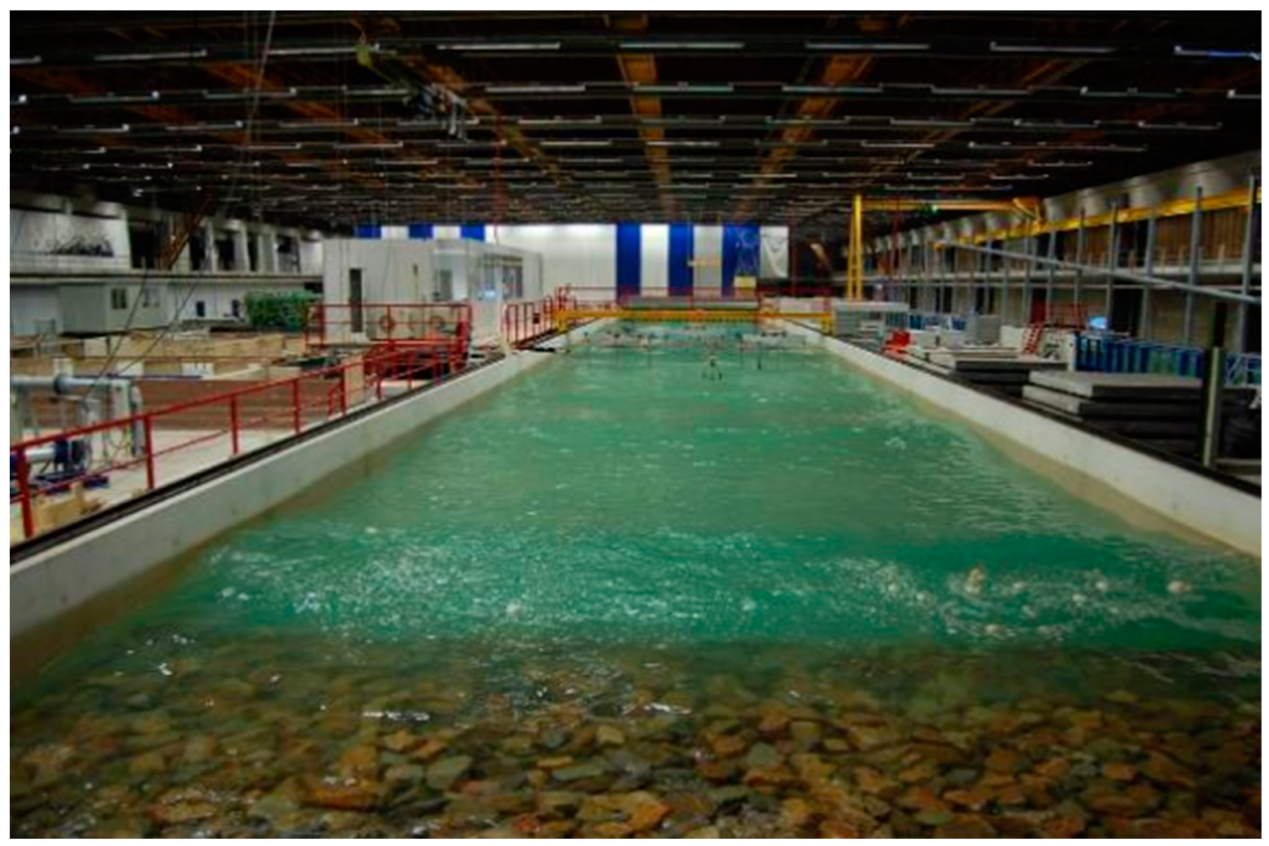
In total, 2 3-week measurement campaigns were undertaken as part of the European Space Agency’s Open Space Innovation Platform programme on the remote sensing of plastic marine litter between 4th October 2021 and 4th February 2022 at the Deltares Atlantic Basin test facility in Delft, The Netherlands. The Atlantic Basin is a large flume, 8.7-m wide and 75 m long, that is capable of generating both waves and currents, as seen in Figure 1.

The difference between the deep water wave conditions and shallow water wave conditions can be represented by the wavenumber (k) times the water depth (d). This value reaches infinity (kd -> ∞) for deep water wave conditions, while it approximates to zero for shallow water waves.

Throughout the measurement campaigns, the gravity wave conditions were varied during multiple tests. To incorporate representative test conditions for the plastics, deep water wave conditions were selected. A wave period (Tp) of 1.2 s and a water depth of 1 m were used, which created a kd factor of 2.8, which is acceptable for simulating deep water wave conditions. As the waves generated in the test facility are limited by the water depth, wave steepness, and acceleration of the wave paddle, it was not possible to increase the kd factor even further.

Tests were carried out for both regular and irregular wave conditions, where the regular waves have almost identical wave heights. In

Table 1. Wave conditions used in the testing campaign for both regular (reg) and irregular (irreg) conditions. The ARC was switched off for higher irregular wave conditions due to limitations of the test facility.

Wave Conditions	$\mathit{T}\mathit{p}$	$\mathbf{Reg}/\mathbf{Irreg}:\mathit{H}\mathit{s}$	ARC		$\mathrm{kd}$
	[s]	[m]	Reg.	Irreg.	[-]
Wave Condition 1	1.2	0.05	on	on	2.81
Wave Condition 2	1.2	0.09	on	on	2.81
Wave Condition 3	1.2	0.17	on	off	2.81

, the wave height and wave period of both the regular and irregular wave conditions are shown. The wave height for the irregular wave conditions represents the significant wave height (Hs: the average of the highest 1/3rd of the waves). This means that the individual waves occurring in the wave spectrum can have larger wave heights than the values reported in Table 1. Irregular waves are important to test and were the main focus of testing, as the natural seaway on the oceans is irregular, where the sea rarely shows a unidirectional, regular sinusoidal wave pattern. Instead, we observed mixtures of different wave lengths, heights, and directions [22].

The plastics were deployed near the wave paddle, and they drifted along the basin due to Stokes drift. The waves generated by the wave paddle were reflected on a permeable wall within the basin and from the end of the basin. The amount of wave reflection was calculated using three wave gauges positioned at fixed intermediate distances. With the measured wave signals at these wave gauges, the mean incoming waves and the mean reflected waves were determined by analysing the timeseries of the three wave gauges. The reflected wave height equalled about 10% of the incoming wave height. This reflected wave was absorbed again at the wave paddle by Active Reflection Compensation (ARC). In this way, the generated wave signal compensated for the reflected waves within the basin.

During the measurement period, the water level, wave height, current velocity, and flow rate were measured by the Deltares facility to ensure that all conditions were strictly met.

A full brief on the test conditions used within the Deltares facility can be found in de Fockert and Baker, 2022 [23].

2.2. Plastic Used

In total, 21 different typologies of plastic items were used during the test campaigns, as can be seen in Appendix A (Table A1).

During the tests, different concentrations of plastics were used. These concentrations are presented in

Table 2. Applied concentrations in the test campaigns. Cx corresponds to different concentrations, i.e., plastic spheres were tested at 9 different concentrations (C01–C09).

PlasticID	Concentration (g/m2)
	C01	C02	C03	C04	C05	C06	C07	C08	C09
Plastic Bottles	40	20	18.4	10	4.6
Fixed Plastic Nets	11.25
Plastic Bottles + Fixed Plastic Nets	83.3
Plastic Straws	10
Plastic Food Wraps and Bags (Marine Litter)	2.3	4.6	8.3
Plastic Nets (Marine Litter)	10
Plastic Nets and Bottles (Marine Litter)	8.3
Plastic Bottles without Caps/Filled with Water	4.6	18.4
Plastic Pellets	20
Styrofoam	10
Plastic Caps and Lids	10
Cigarette Filters	10
Plastic Cutlery	14
Plastic Spheres	2	4	6.4	10	20	40	80	120	153
EVA Cylindrical Foam	10
Transparent Plastic Lids	10
Transparent Plastic Lids without Edges	10

. During some tests, the concentrations were manually increased to reach a specific concentration in the area of interest. These cases are represented with multiple concentrations in Table 2.

2.3. Test Procedures

Reference measurements were taken to test the capability of floating plastic to change the backscattering of radar. The reference measurements consisted of defined wave conditions within the tank, but with no plastic items in the water. The test measurements consisted of the exact same wave conditions, but with the plastics added into the water.

During the first measurement campaign, reference measurements were taken of all wave cases in a day. These were then used as the references that all test measurements were compared against for their respective wave heights. During the second measurement campaign, a test protocol was established to ensure reference measurements and test measurements could be taken within each experiment at the shortest possible distance in time (i.e., references for each test were taken within 40 min before the test acquisitions began).

The plastic spheres were released into the basin through an automated manner by a sphere dispenser. This dispenser released the spheres at a fixed interval with a specific dispenser seed. In this way, the required concentrations could be controlled more accurately.

Except for the plastic spheres, all other plastics were manually distributed in the test facility. Prior to each test, the total amount of added plastic was carefully weighed, and this amount was constantly fed into the Atlantic Basin from the wave pedal located 16.7 m behind the measurement set-ups. This created a homogenous spread of plastic concentration throughout the different measurement areas.

At the end of each test, the particles were removed from the basin to ensure no contamination of plastics were present between the tests and references.

The first measurement campaign conducted in October 2021 consisted of a variety of tests on different types of plastics and wave conditions to understand the initial capabilities of the radar set-up. From these results, the second measurement campaign conducted between January and February 2022 had more focussed testing on fewer wave conditions and plastics.

2.4. Measurement Equipment Set-Up

The measuring equipment consisted of a ground-radar, where the back end is an Anritsu Site Master S820e Vector Network Analyser. It is connected to C- and X-band antennas. The specifications of the hardware can be seen in

Table 3. Measuring equipment specifications for ground radar used to measure Deltares campaign experiments.

Equipment	Frequency Range	Polarisation	3dB Beamwidth	Dynamic Range
Anritsu Site Master S820e VNA	1 MHz–14 GHz	-	-	110 dB from 20 MHz to 14 GHz
C-Band Antenna	5–6 GHz	Quad-pol	25°(H)/15°(E)	-
X-Band Antenna	8.2–12.4 GHz	Single VV Pol	16°(H)/14°(E)	-

. A solid-state switch was used to perform the quad polarimetric acquisitions using the single input and output ports of the VNA. Semi-rigid cables (DC to 18 GHz) were strapped in position to minimise the changes between the acquisition days.

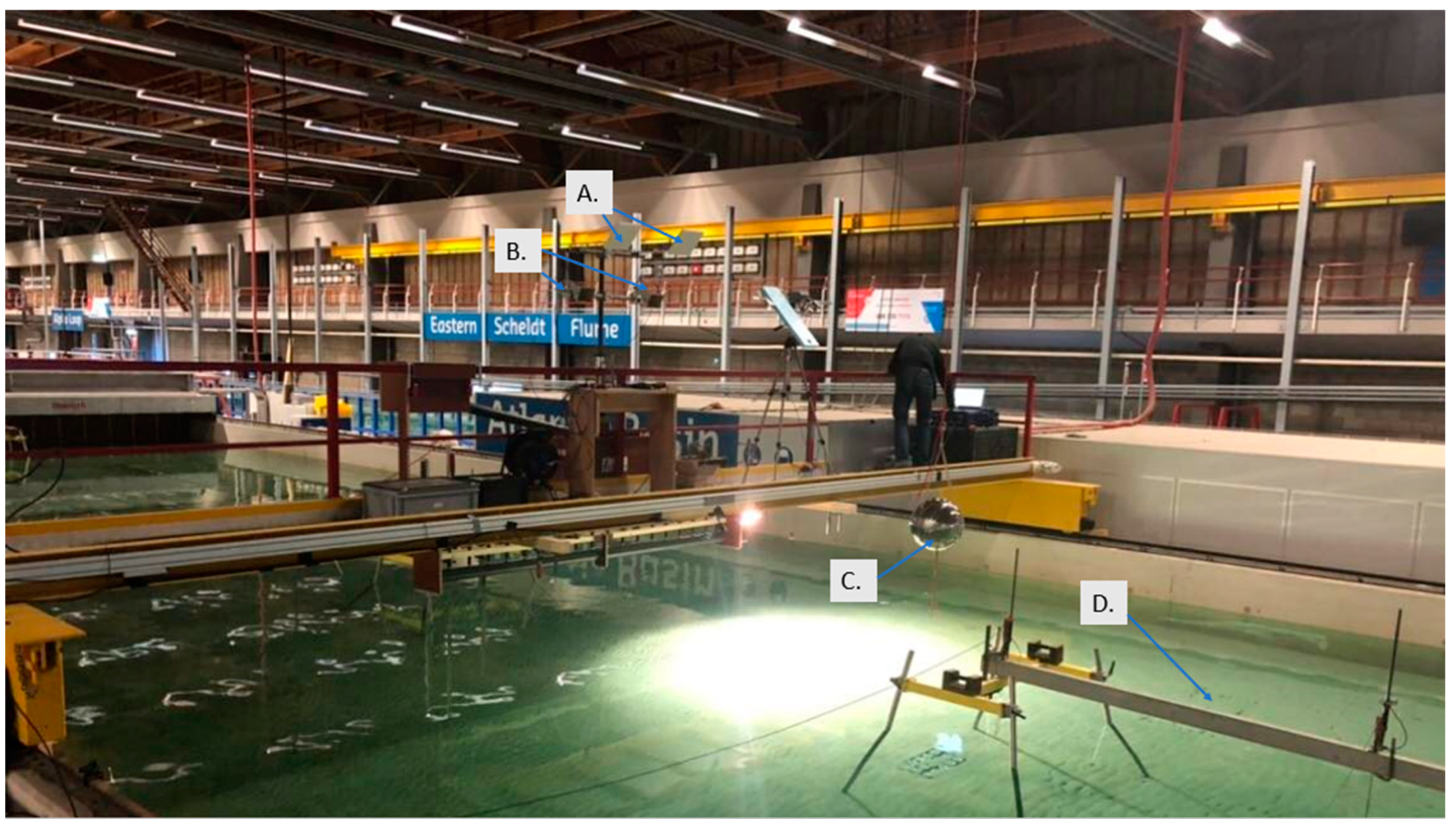
The radar equipment was located on the bridge that crossed the middle of the Atlantic Basin. The C-band antenna (Figure 2A) was located 4.04 m above the floor of the basin and the X-band antenna (Figure 2B) was located 3.61 m above the floor of the basin. An external sphere used as a target for calibrating the polarimetric behaviour (further details in Image Formation) was located 2.5 m in front of the radar. The radar was looking downstream with an incidence ranging between 30° and 50°. For both frequencies, the 3 dB main lobe formed a footprint in cross-range that was approximately 2 m. The sweeps in frequency considered 1 GHz (for each band), which resulted in a theoretical range resolution of 15 cm.

2.5. Image Formation

The radar architecture is a Step Frequency Continuous Waveform (SFCW), where the transmitting wave was sweeping as a linear frequency modulation in a desired bandwidth. The received signal was then processed including a Hamming window and inverse Fourier transform to focus the range profile. Each VNA sweep, therefore, produced a single range profile. The C-band antennas considered a sweep between 5 GHz and 6 GHz, while the X-band antennas considered a sweep between 9.5 GHz and 10.5 GHz. These frequency ranges were chosen to be inclusive of the bandwidths used by SAR satellites. The radar parameters were set so that the range of ambiguity was 80 m. This was to ensure that returns from the back of the 75 m tank were not overlapping with our test area due to ghosts (please note that the bridge with the radar was around the middle of the tank).

Each experiment consisted of monitoring a type and concentration of plastic (or the reference for this). In each experiment, we acquired several repetitions in time. This means that each acquisition considered multiple sweeps over the course of the experiment. The minimum number of sweeps used was 80 and the maximum was 580, and this duration depended on factors such as the permanency of plastic in the radar beam and the amount of plastic available for the experiment.

The calibration was conducted keeping in mind two main goals: (a) backscattering stability and (b) radiometric accuracy. It is known that VNA signal generators may drift in amplitude and phase during a measurement campaign since they may be dependent on temperature and humidity, as well as other factors [24]. The fact that references were taken up to forty minutes before the tests should not lead to large drifts in the temperature and humidity, and, therefore, should not lead to drifts in the VNA. However, calibration was still necessary to more easily compare the results between the different acquisition days, and to create reassurance that any potential drift was mitigated. For this reason, we identified a permanent target inside our radar profile and used this as a reference to clip all of the radar profiles (for a given frequency and polarisation) together. The permanent “target” for the C-band experiment was the antenna leak between the transmitter and receiver. The target for the X-band experiments was a reflection from the bridge straight below the antennas. Since the radar geometry was fixed over the entire campaign, these two returns showed a remarkable stability.

In order to calibrate the polarimetric behaviour and to provide a measure that could be exported to other experiments, we wanted to calibrate the profile radiometrically over a canonical target. An external 30 cm metal sphere was used to further convert the clipped images into radar cross sections. The sphere did not have any impact on clipping the same polarisation channel since the radiometric calibration was a range independent factor given a band and a polarisation channel. It, however, affected the weight when comparing the frequencies and polarisations channels.

2.6. Scattering Model Hypothesis for Marine Plastics

In this section, we introduce the scattering model that we hypothesise for plastic in water.

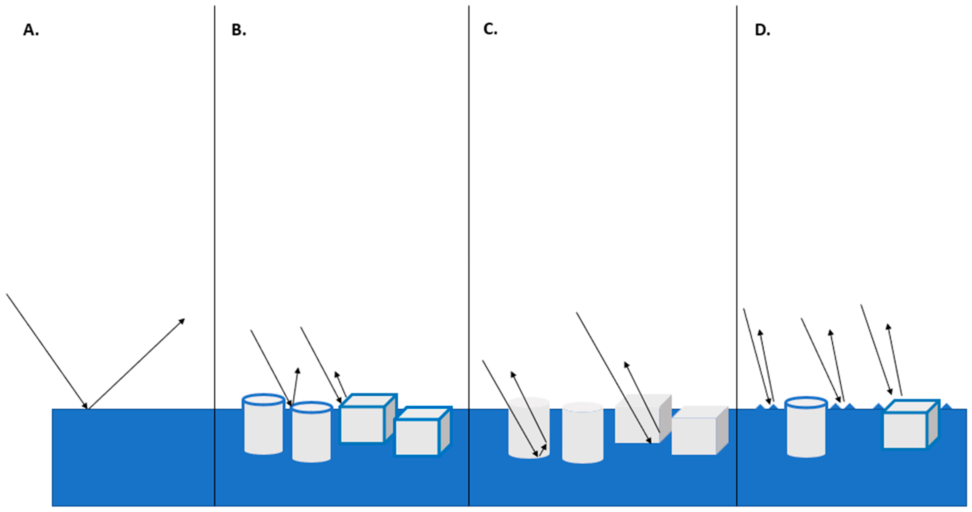
We hypothesise three different scattering mechanisms that could contribute to the total scattering coming from plastic in water: Direct, Indentation, and Wave-Generation. We assume that these are all present, but their contribution may be very different when, in some conditions, one can strongly dominate over the others.

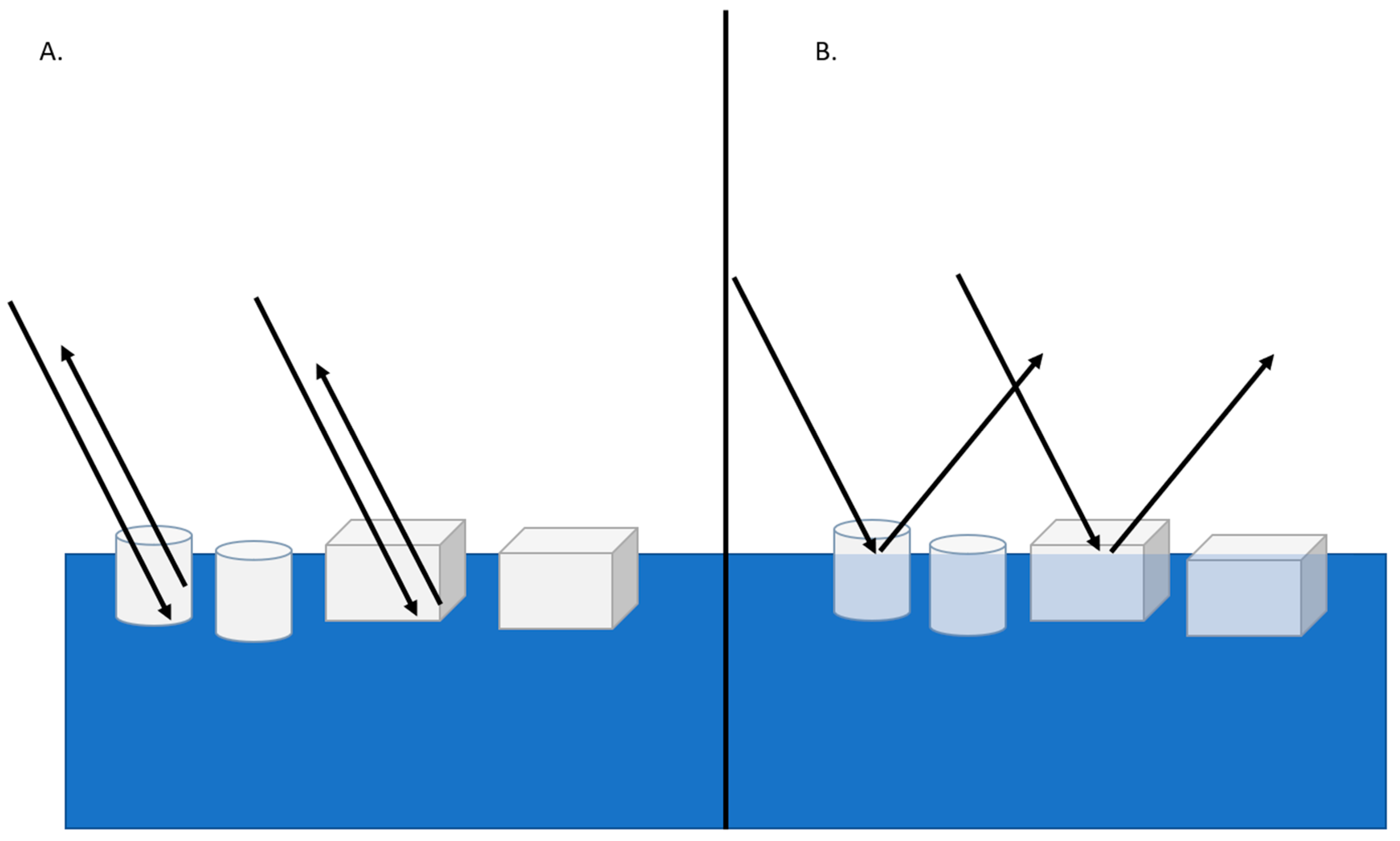
Scattering is strongly dictated by the dielectric constant, together with other factors including roughness, shape, and size. The real part of the dielectric constant is related to the amount of power of the induced current on the object and, therefore, the amount of scattering. For plastic, the relative dielectric constant is relatively small (proximal to one, the one of air). Therefore, we do not expect plastic to scatter directly. However, when water is included in the scene there are different phenomena that can be triggered and we hypothesise three mechanisms that can provide an increased backscattering compared to clean water, as seen in Figure 3.

Water with no plastic has a smooth surface, calling for specular reflection of the signal. This can be easily demonstrated looking at SAR images since those areas appear as dark.

Whether or not the radar waves penetrate any medium is controlled by the imaginary part of the dielectric constant of the particular medium. A medium with a high imaginary part of the dielectric constant, such as water, is mostly impenetrable (mm or cm penetration depth depending on several factors, including frequency and salinity). Therefore, when a thin layer of liquid water is on top of the plastic, it creates a change in the surface roughness due to the raised ‘bumps’ of liquid water. The backscattering from these “bumps” should be increased due to the fact that water also has a high real part of the dielectric constant. Here, we call this ‘direct scattering’. The thickness of the liquid water layer can be very small, with just 1 mm being potentially sufficient, as shown by observations of wet ice, snow, or icebergs [25,26,27]. On the other hand, when the imaginary part of the dielectric constant is low, the medium can be penetrated easily without loss, as is the case for plastic. The plastic, therefore, is penetrated; however, it is still producing an effect on the water underneath by producing indentations and extra roughness, which we call ‘indentation scattering’. This extra roughness induces a scattering from the surface (as if extra capillary waves were present).

While the figure above is an example on still water, the physical mechanisms remain the same in moving water. Finally, another mechanism was also observed during testing, where capillary waves were generated from plastic items interacting with moving water throughout every test. Different items produced differing disturbances on the water surface, but all plastic items generated amounts of capillary waves on the water surface as the waves crashed on them. This is an interesting observation as radar is sensitive to the surface roughness and differences in the capillary wave generation can potentially be detected. Here, we call this ‘wave-generation’ scattering.

To summarise, these three scattering mechanisms can all be present at the same time, although we expect that one will dominate over the others depending on the frequency used, size of plastic, buoyancy, waves, wind, rain, and other factors.

2.7. Radar Data Analysis

The analysis we performed focussed on the signal intensity (or backscattering). The intensity (in dB scale) was taken from all focussed and calibrated acquisitions during the run of each experiment (Reference or Test).

The following information is displayed in two main ways for each experiment. First, the mean of the intensity (dB) was evaluated by averaging all of the repetitions. This trend was plotted against the distance (m), allowing us to average out the signal variation due to speckle. Second, images were created where the two dimensions represent the distance from the radar (no. of pixels) vs. time (no. of acquisitions taken). The image colour represents the intensity on a linear scale. These images are often referred to as radargrams (e.g., when dealing with ground-penetrating radars). Although radargrams are affected by speckle, they contribute to the qualitative understanding of the experiments from each measurement session. They also help to gain insights into the time dynamics of the backscattering, which helps the interpretation.

The visualisation itself is a good way to qualitatively compare backscattering differences between the test (waves and plastic) and reference (same waves/no plastic) experiments.

To create a quantitative insight into the data, a statistical analysis was undertaken. Each test measurement underwent a statistical analysis. Starting from the radar profile, we identified the ROI representing water in the tank where plastic would drift through. The pixels in that area were averaged over time to obtain a single mean value for the ROI. This mean value was then compared against the same ROI during the reference acquisition, which considered the same wave conditions but with no plastic presence.

We applied our statistical test for:

• Null Hypothesis H0: No change in the mean backscattering
• Alternative Hypothesis H1: Change in the mean backscattering

Using the Central Limit Theorem (CLT), we assumed the distributions of the differences of the sample means approximated a normal distribution. All sample sizes were greater than 80 (the minimum requirement considered sufficient for the CLT to hold is often stated as 30).

The threshold for H1 (i.e., confidence interval) can, therefore, be set using a Neyman-Pearson-derived constant false alarm rate (CFAR) methodology which only required the knowledge of the mean and standard deviation [28]. The threshold was set as: difference of the mean > 3 * standard deviation. This threshold led to a confidence interval of 99.7%, and since this is a one-trail test, the corresponding false alarm rate was around 0.15%. This confidence interval was subject to the assumption of normal differences.

This statistical analysis was applied to all experiment cases that were undertaken over the test campaigns. From this, tables were then created showing if the statistical differences were or were not found in all of the experiments that were undertaken.

When dealing with SAR images, one traditional processing step is speckle filtering. This can be easily conducted using a boxcar filter. When we analyse the data as described above, this could be compared to using single-look complex (SLC) Synthetic Aperture Radar (SAR) data. However, when applying a boxcar, this could be compared to using Ground Range Detected (GRD) SAR data (as provided by the ESA Sentinel-1 satellite), where multi-looking is present. The boxcar filter was applied to time vs. distance radar imagery to reduce the noise present within the images. The boxcar reduces the overall variation present in an image by setting each pixel’s intensity equal to the average of its neighbour. The boxcar filter we used for these acquisitions was 5 × 1 (Time × Space). This allowed us to not lose any range resolution during this process.

Applying the boxcar filter to the test reduces the standard deviation of the difference (test vs. reference) and, therefore, modifies the final threshold. This is equivalent to saying that the boxcar filter reduces the noise level in the image, so we can use a lower threshold to monitor the differences without impacting the false alarm rate.

We did not perform any coherent polarimetric analysis, since the moving of targets (waves and plastic) during the acquisitions resulted in decorrelating the polarimetric channels and, therefore, not allowing coherent polarimetric analysis (the covariance matrices are diagonal over the targets of interest). In the following, in C-band, the different polarimetric channels are compared using intensities only, in the same way that some satellite systems do no acquire polarimetric data coherently (e.g., some modes of COSMO-SkyMed or NOVASAR).

3. Results

Multiple plastic items were used as free-floating targets in different experiments. In the first part of this section, we showed the results of plotting the backscatters in different test cases between the reference and experiment. For the sake of brevity, the graphs showed here only cover very limited selected cases, which can be used to demonstrate the trends. The second part of this section includes the statistical analysis that covers every single test we performed.

3.1. Free-Floating Targets: X-Band—Intensity Plots

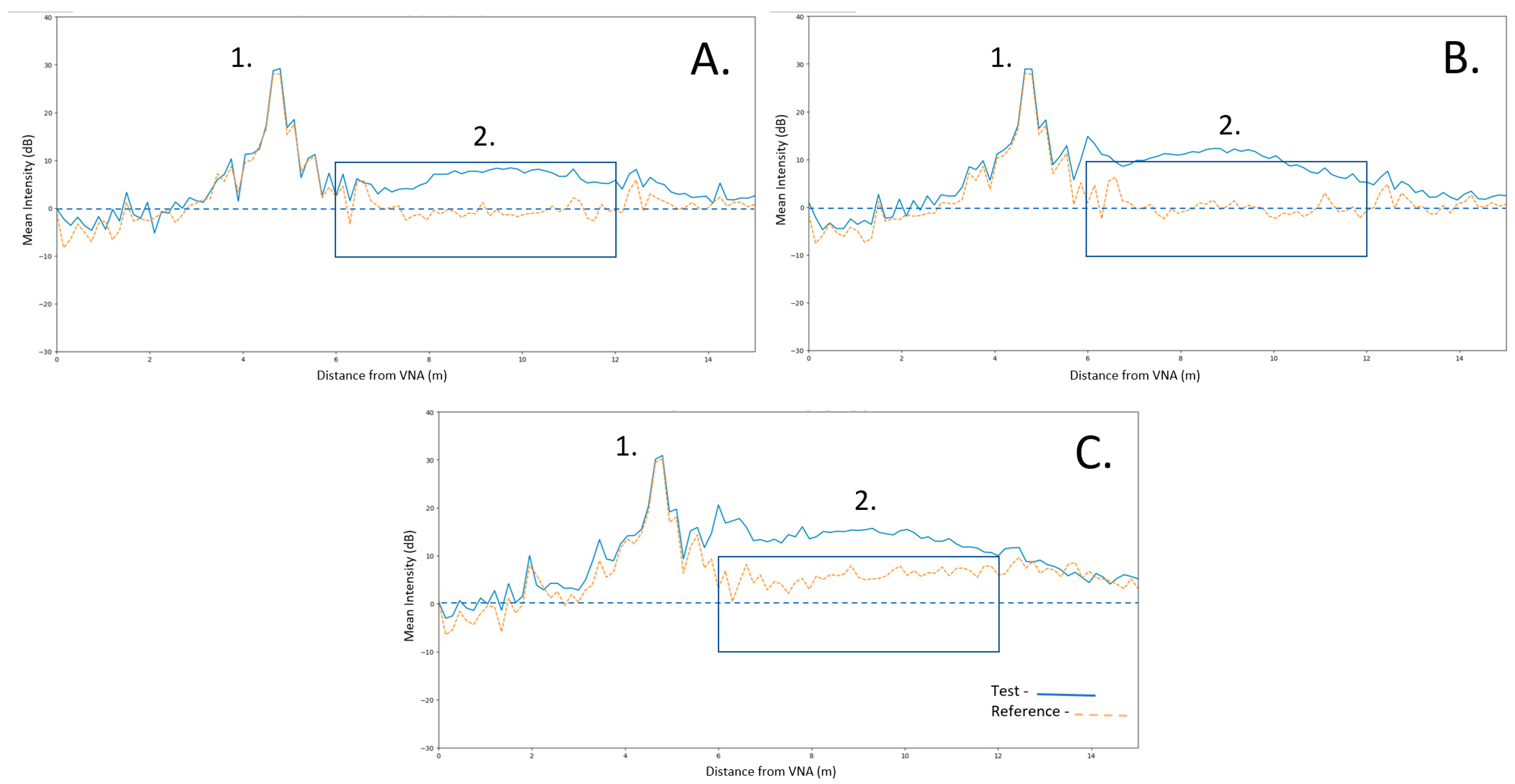
The following line graphs show the X-band frequency results. All measurements were made between 9.5 GHz and 10.5 GHz frequency ranges in VV polarisation. The mean intensity was taken from all acquisitions during the experiment. The distance was measured considering the VNA as the starting point. In the figure below, we see three experiments comparing test and reference acquisitions. We see a peak of intensity from the lip of the bridge, labelled ‘1.’ and a blue box labelled ‘2.’ which highlights our ROI within the wave tank, and, finally, a dashed line, which is used as an arbitrary reference line to aid visualisation.

In Figure 4, we see a comparison of the backscatter from the reference acquisitions with no plastic in the water and the test acquisitions with different plastics inside the water. Please note the stability of the reference point over the peak one. The mean over two bins was used to clip the images to avoid errors due to micromovements and fractional pixels. This is when the same target (the bridge edge) appeared as a fractional pixel over two bins. For A, an increase in intensity by 8.1 dB (around 6 times in linear) can be seen from the test acquisition, where the only change between the test and reference experiments was the addition of plastic bottles into the water. For B, an increase in intensity by 10.9 dB (around 15 times in linear) can be seen from the Test acquisition, where the only change between the test and reference experiments was the addition of cylinder foam into the water. In C, due to the increased height of the waves used in this experiment, in tandem with 17 cm waves having more breaking waves, we see an overall increase in backscattering from our reference when compared with the 9 cm waves references. We can also see an increase in intensity by 7.3 dB (around 4 times in linear) from the test acquisition, where the only change between the test and reference experiments was the addition of plastic lids into the water.

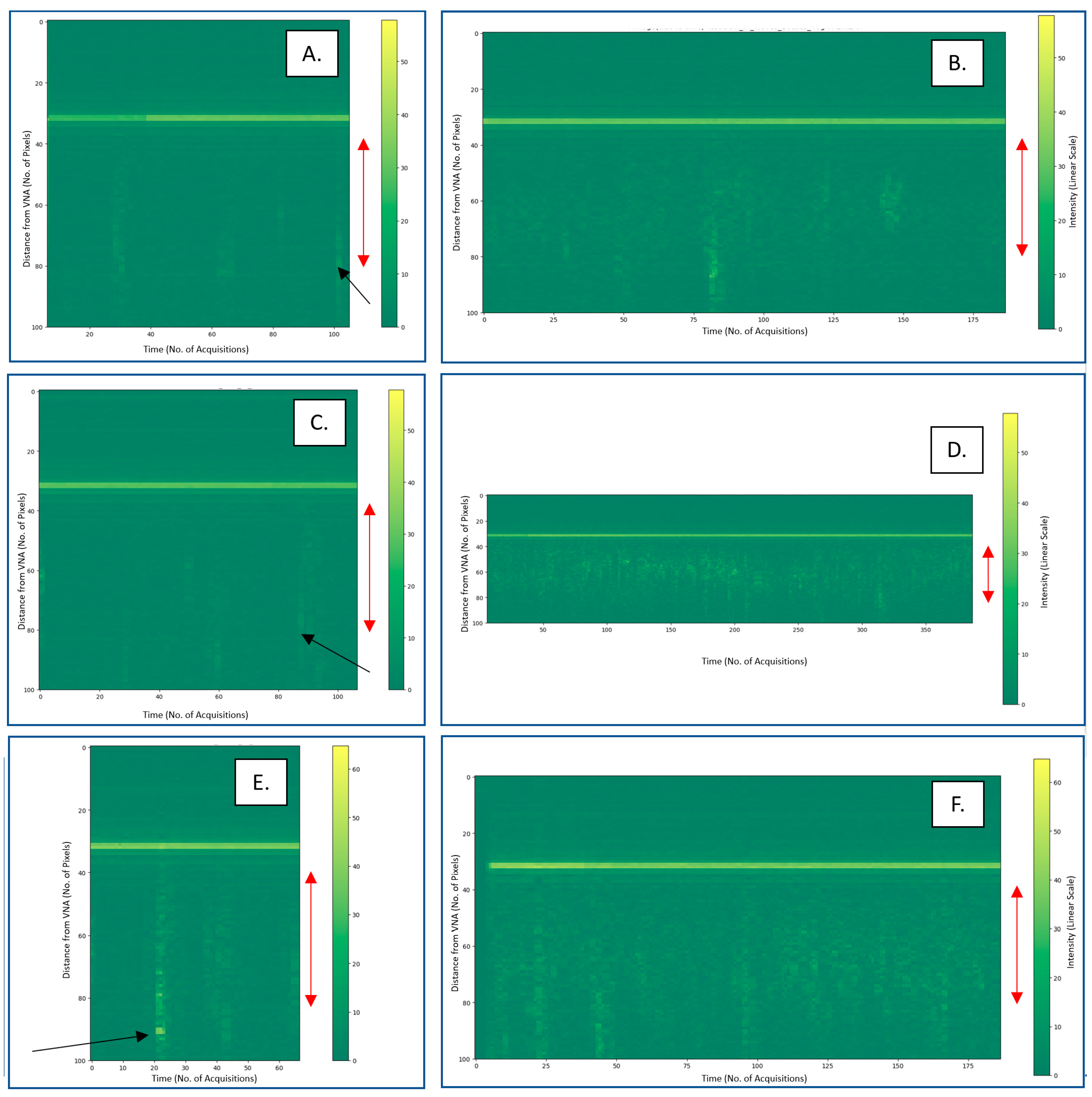
To create a time series of this intensity data, radargrams were created. Within the figures, we highlighted the colour gradient showing the intensity on a linear scale. The black arrows on the figures highlighted a feature of interest. These figures are shown in the figure below.

In Figure 5, we see the radargram comparisons of the backscatter from the reference acquisitions with no plastic in the water and the test acquisitions with different plastic items moving through the water. The region that the radar can see is indicated by the red double arrow. However, we are not including all of this in our analysis since the incidence angle in that region outside the double arrow was very shallow, above 50°, and it is not suggested to use those regions to monitor plastic. Note that most satellites tend to not acquire incidence angles over 50° because these angles are too shallow for almost any Earth observation activity [29]; the SAR Satellite Sentinel-1 acquires with an incidence angle range of 29.1–46.0° [30]. Although we exclude them in the statistical analysis, it is interesting to observe how they can still show a qualitative difference between the presence and absence of plastic.

A change in the intensity with plastic can be seen in the radargrams, with a more uniform layer of increased intensity seen from the test experiments with plastic items moving through the tank. Most of the scattering from plastic comes from the ROI, although we still see some increase even further away with very shallow incidence angles, but the difference is very evident when plastic is introduced.

We would also like to draw attention to the feature identified by the black arrows in Figure 5. We see these features in other tests and comment on these later in the paper.

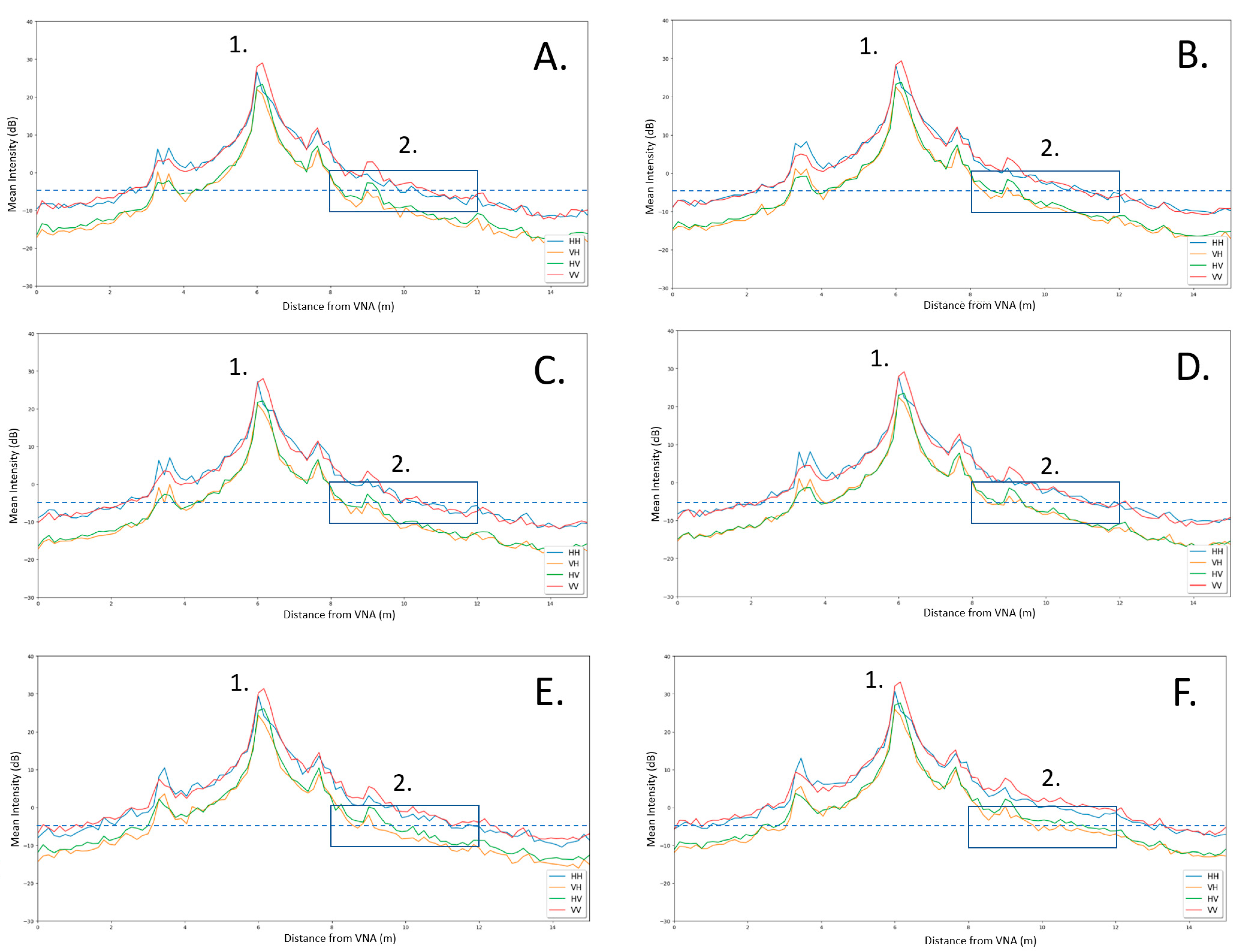
3.2. Free-Floating Targets: C-Band—Intensity Plots

The following line graphs show the C-band frequency results obtained from the same setting as the X-band results. All measurements were made between the 5 GHz and 6 GHz frequency range in quad-polarisation (VV, VH, HV, HH), where H stands for linear horizontal and V stands for linear vertical. The mean intensity was taken from all acquisitions during the experiment. The distance was measured from the VNA as a starting point. We display the same tests as the X-band cases to serve consistency; however, for clarity we have separate graphs for reference and test acquisitions.

In Figure 6, we can see a comparison of the backscatter from the reference acquisitions with no plastic in the water and the test acquisitions with different plastic items moving through the water. An increase in intensity can be seen in all polarisations from the test acquisition. For A, these intensity increases were: 1.03 dB for VV, 1.68 dB for VH, 1.29 dB for HV, and 1.99 dB for HH. For B, the intensity increases were: 1.86 dB for VV, 2.51 dB for VH, 1.96 dB for HV, and 1.61 dB for HH. For C, the intensity increases were: 2.54 dB for VV, 3.69 dB for VH, 2.91 dB for HV, and 2.48 dB for HH. These increases are much smaller when compared with the differences in intensity found within the X-band experiments.

Please note how the co-pol channels (HH and VV) were always higher than the cross-pol channels (HV and VH). Additionally, HV and VH were not identical due to two reasons: the antennas beamwidths in the H and E plane were not identical and the noise levels were different in the two channels.

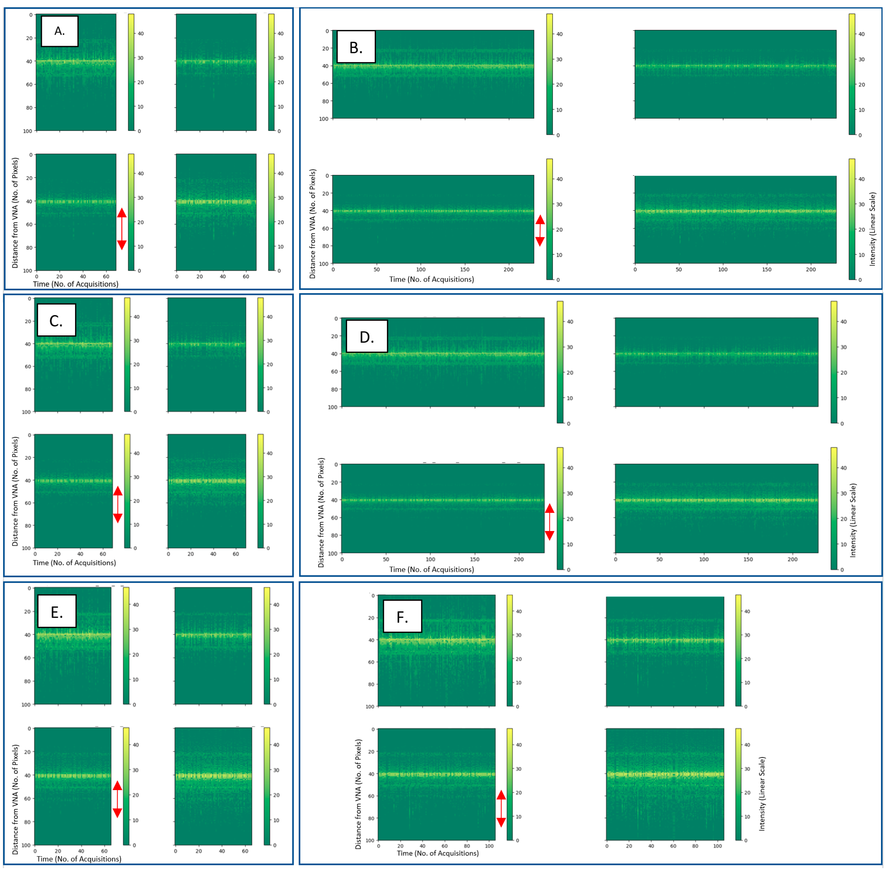
To create a time series of this intensity data, radiograms were created. These are shown below.

In Figure 7, we can see a comparison of the backscatter from the reference acquisitions with no plastic in the water and the test acquisitions with plastic moving through the water. It is difficult to see a distinctive change in the intensity over time in the radargrams when comparing the test acquisitions to their respective reference. However, there is a small difference evident in Figure 7C where an increase in intensity can be seen from when the plastic lids were flowing through the tank.

3.3. Statistical Analysis

We applied our statistical test for:

• Null Hypothesis H0: No change in the mean backscattering
• Alternative Hypothesis H1: Change in the mean backscattering

The results of the statistical analysis on each test were formatted into tables (as seen below). The results showed here use a confidence interval of 99.7% and a corresponding false alarm rate of around 0.15% as this is a one-trail test. For this testing, our hypotheses are as follows:

• Null Hypothesis H0: No change in the mean backscattering between the test and reference acquisitions.
• Alternative Hypothesis H1: A change in the mean backscattering between the test and reference acquisitions.

This testing was conducted on the data with and without the use of the boxcar filter.

3.4. Without Boxcar

The results from

Table 4. Results of statistical analysis undertaken on 1st campaign measurements without the use of a boxcar filter. Values filling the table are the results of the difference of the reference measurement and test measurement in a linear format. Any value in green shows that the alternative hypothesis was fulfilled; any value in orange shows that the null hypothesis was fulfilled.

Without Boxcar Filter						C-Band				X-Band
Date	Objective	Wave Pattern	Hs [cm]	Plastics	Concentration [g/m2]	HH	HV	VH	VV	VV
14 October 2021	Plastics at Fixed Position	No	0	Nets	11.25	0.18	0.05	0.07	0.08	4.93
				Nets + Bottles	83.3	0.6	0.33	0.38	0.48	13.3
		Irregular	9	Nets	11.25	0.03	−0.02	0.02	−0.02	−4.71
				Nets + Bottles	83.3	0.09	0.04	0.06	0.08	13.9
15 October 2021	Plastics at Fixed Position	Irregular	17	Nets	11.25	0.02	0.04	0.05	0.03	−2.32
				Nets + Bottles	83.3	0	0	0.04	0	9.65
18 October 2021	Variations in Free-Flowing Plastics	Irregular	9	(New PET Bottles)	4.6	0.15	0.08	0.06	0.16	0.92
					40	0.17	0.08	0.08	0.17	6.36
				Organic Plastics (Sheets)	2.3	1.38	0.85	0.57	1.59	1.85
					4.6	1.39	0.88	0.8	1.84	4.21
19 October 2021	Variations in Free-Flowing Plastics	No	0	Pellets	20	1.6	0.88	0.82	1.69	0.87
				(New) PET Bottles Partly Submerged	4.6	−0.04	0.01	0.01	0.04	−0.12
					18.4	0.04	0.01	0.02	0.03	−0.45
		Irregular	9	Wrapped Fishing Nets/Ropes with Bottles	8.3	−0.02	−0.02	−0.02	−0.04	−1.86
				Partly Submerged Bottles	46	−0.15	−0.12	−0.04	−0.23	0.78
20 October 2021	Variations in Wave Conditions	Irregular	5	Plastic Sheets and Bags (Nets/Ropes with Bottles)	8.3	0.62	0.42	0.44	0.97	3.93
				Wrapped Fishing Nets/Ropes with Bottles	8.3	0.68	0.43	0.51	1.06	3.99
			9	Sheet Materials	8.3	0.76	0.36	0.46	0.73	2.77
			17	Sheet Materials	8.3	0.48	0.3	0.42	0.77	0.92
		Irregular and Capillary	17	Wrapped Fishing Nets/Ropes with Bottles	8.3	0.49	0.29	0.39	0.66	−2.38
				Sheet Materials	8.3	0.27	0.23	0.27	0.58	−2.11
21 October 2021	Capillary Waves	Irregular and Capillary	5	Sheet Materials	8.3	0.64	0.31	0.42	0.77	0.22
				Nets/Ropes	8.3	0.68	0.43	0.5	1.06	3.9
			9	Sheet Materials	8.3	−0.02	−0.02	0	−0.05	3.84
				Nets/Ropes with Bottles	8.3	−0.03	−0.05	−0.07	−0.02	−1.74
	Variations in Free-Flowing Plastics	Irregular	9	Styrofoam	10	0.18	0.03	0.05	0.03	1.11
				Lids/Caps	10	0	−0.03	0.01	−0.1	0.31
				Cigarette Filters	10	0.09	−0.02	0	−0.05	−0.26
22 October 2021	Variations in Free-Flowing Plastics	Irregular	9	Cutlery	14	1.9	0.83	0.7	1.4	1.89

indicate that statistically significant differences were found in only 2/29 cases between the test and reference acquisitions in the C-band data, in HH- polarization for plastic cutlery, and in VV-polarization for plastic sheets, both in 9 cm waves. A statistically significant difference was found in 7/29 cases between the test and reference acquisitions in the X-band data. It can be noted that three of the X-band measurements with a statistical difference involved the use of fixed position targets of plastic, making the detection of any differences much easier.

The results from

Table 5. Results of statistical analysis undertaken on 2nd campaign measurements without the use of a boxcar filter. Values filling the table are the results of the difference of the reference measurement and test measurement in a linear format. Any value in green shows that the alternative hypothesis was fulfilled; any value in orange shows that the null hypothesis was fulfilled.

Without Boxcar Filter						C-Band				X-Band
Date	Objective	Wave Pattern	Hs [cm]	Plastics	Concentration [g/m2]	HH	HV	VH	VV	VV
26 January 2022	Free-Floating Plastics	Irregular	9	Spheres [2 cm] in Lines	6.4	−0.08	−0.04	−0.04	−0.08	1.14
					40	−0.09	−0.04	−0.03	−0.1	0.94
					80	−0.06	−0.02	−0.06	−0.1	1.05
					120	0.01	−0.01	0.08	0	1.18
					153	−0.12	0	−0.01	0.04	1.23
27 January 2022	Free-Floating Plastics	Irregular	9	Spheres [2 cm] with Holes Taped	2	−0.02	0	0.04	0.04	0.19
					4	0.08	0.05	0.01	0.08	−0.09
					6.4	0.12	0.05	0.03	0.1	0.15
					20	0.05	0.04	0.04	0.09	0.14
	Full 9 cm Reference			No Plastic	0	0.13	0.03	0.05	0.11	0.37
28 January 2022	Free-Floating Plastics	Irregular	9	Bottles	20	0.1	0.04	0.05	0.06	0.95
				Bottles	40	0.12	0.06	0.04	0.11	0.94
				Straws (24 cm)	20	0.1	0.05	0.05	0.06	4.06
				Cylinder Foam (20 cm)	20	0.12	0.07	0.09	0.14	2.68
				Cylinder Foam (10 cm)	20	0.19	0.1	0.13	0.18	1.94
31 January 2022	Free-Floating Plastics	Irregular	9	Cylinder Foam (5 cm)	20	0.12	0.02	0.03	0.08	2.17
				Straws (12 cm)	20	−0.01	0.01	0.01	−0.01	0.85
				Straws (6 cm)	20	0.01	−0.01	0	−0.04	0.18
1 February 2022	Free-Floating Plastics	Irregular	9	Spheres [2 cm] with holes Taped	10	0.2	0.06	0.08	0.1	0.49
			17		10	0.14	0.05	0.06	0.08	−0.12
					20	0.11	0.04	0.08	0.14	0.19
					40	0.2	0.11	0.07	0.17	−0.03
2 February 2022	Free-Floating Plastics	Irregular	5	Spheres	10	0.2	0.09	0.05	0.17	0.26
					20	0.02	0.06	0.1	0.19	0.53
					40	0.17	0.1	0.06	0.21	0.35
				Plastic Lids	10	0.38	0.29	0.25	0.53	3.38
			9			0.02	0.01	0.08	0.06	2.18
			17			0.27	0.27	0.16	0.45	2.79
3 February 2022	Free-Floating Plastic	Irregular	5	Bottles	20	0.17	0.1	0.08	0.21	1.38
						-	-	-	-	1.38
	Full 5 cm Reference			No Plastic	0	0.1	0.04	0.06	0.09	0.32
	Free-Floating Plastics		9	Bottles	20	0.02	0	0.01	0.07	1.07
			17			0.02	0.01	−0.01	0	−0.03
	Full 17 cm Reference			No Plastic	0	0.02	−0.03	−0.02	−0.06	−0.5
4 February 2022	Free-Floating Plastics	Irregular	9	Bubble Wrap	1 m Long Strip	-	-	-	-	1.63
				Plastic Lids (No Edges)	10	0.05	0.02	0.03	0.05	3.28
			17			0.06	−0.03	−0.04	−0.01	1.75

indicate that statistically significant differences were found in only 1/37 cases between the test and reference acquisitions. This was found in the X-band frequency: 5 cm wave height plastic lids (10 g/m²). The C-band acquisitions had no cases where a statistically significant difference was found between the test and reference acquisitions in any of the experiments. The experiments that were undertaken to eliminate changes in the wave machines’ production of waves also showed that there were no significant differences between the wave conditions during reference acquisitions when compared with test acquisitions.

3.5. With Boxcar

The results from

Table 6. Results of statistical analysis Undertaken on 1st campaign measurements with the use of a boxcar filter. Values filling the table are the results of the difference of the reference measurement and test measurement in a linear format. Any value in green shows that the alternative hypothesis was fulfilled; any value in orange shows that the null hypothesis was fulfilled.

With Boxcar Filter						C-Band				X-band
Date	Objective	Wave Pattern	Hs [cm]	Plastics	Concentration [g/m2]	HH	HV	VH	VV	VV
14 October 2021	Plastics at Fixed Position	No	0	Nets	11.25	0.18	0.05	0.07	0.08	4.93
				Nets + Bottles	83.3	0.6	0.33	0.38	0.48	13.3
		Irregular	9	Nets	11.25	0.03	−0.02	0.02	−0.02	−4.71
				Nets + Bottles	83.3	0.09	0.04	0.06	0.08	13.9
15 October 2021	Plastics at Fixed Position	Irregular	17	Nets	11.25	0.02	0.04	0.05	0.03	−2.32
				Nets + Bottles	83.3	0	0	0.04	0	9.65
18 October 2021	Variations in Free-Flowing Plastics	Irregular	9	(New PET Bottles)	4.6	0.15	0.08	0.06	0.16	0.92
					40	0.17	0.08	0.08	0.17	6.36
				Organic Plastics (Sheets)	2.3	1.38	0.85	0.57	1.59	1.85
					4.6	1.39	0.88	0.8	1.84	4.21
19 October 2021	No	No	0	Pellets	20	1.6	0.88	0.82	1.69	0.87
	Variations in Free-Flowing Plastics			(New) PET Bottles Partly Submerged	4.6	−0.04	0.01	0.01	0.04	−0.12
					18.4	0.04	0.01	0.02	0.03	−0.45
		Irregular	9	Wrapped Fishing Nets/Ropes with Bottles	8.3	−0.02	−0.02	−0.02	−0.04	−1.86
				Partly Submerged Bottles	46	−0.15	−0.12	−0.04	−0.23	0.78
20 October 2021	Variation in Wave Conditions	Irregular	5	Sheet Material	8.3	0.62	0.42	0.44	0.97	3.93
				Wrapped Fishing Nets/Ropes with Bottles	8.3	0.68	0.43	0.51	1.06	3.99
			9	Sheet Material	8.3	0.76	0.36	0.46	0.73	2.77
			17	Sheet Material	8.3	0.48	0.3	0.42	0.77	0.92
		Irregular and Induced Capillary	17	Wrapped Fishing Nets/Ropes with Bottles	8.3	0.49	0.29	0.39	0.66	−2.38
				Sheet Material	8.3	0.27	0.23	0.27	0.58	−2.11
21 October 2021	Capillary Waves	Irregular and Induced Capillary	5	Sheet Material	8.3	0.64	0.31	0.42	0.77	3.35
				Nets/Ropes	8.3	0.68	0.43	0.5	1.06	3.9
			9	Sheet Material	8.3	−0.02	−0.02	0	−0.05	3.84
				Nets/Ropes with Bottles	8.3	−0.03	−0.05	−0.07	−0.02	−1.74
	Variations in Free-Flowing Plastics	Irregular	9	Styrofoam	10	0.18	0.03	0.05	0.03	1.11
				Lids/Caps	10	0	−0.03	0.01	−0.1	0.31
				Cigarette Filters	10	0.09	−0.02	0	−0.05	−0.26
22 October 2021	Variations in Free-Flowing Plastics	Irregular	9	Cutlery	14	1.9	0.83	0.7	1.4	1.89

indicate that statistically significant differences were found in 17/31 cases between the test and reference acquisitions in the C-band data with a boxcar filter applied. A statistically significant difference was found in 23/31 case between the test and reference acquisitions in the X-band data with the filter applied. Here, we can see that nearly all test cases using sheet material were found to have significant differences. We can also see that our smaller items, such as lids/caps and cigarette filters, still produced no significant difference in backscattering. Another notable point is that tests using identical materials but with induced capillary waves showed that with induced capillary waves we cannot detect a significant difference in backscattering for the higher wave conditions (9 cm and 17 cm waves). The only test cases where the statistical difference was detectable with induced capillary waves was the sheet material (8.3 g/m²) and nets/ropes (8.3 g/m²) in 5 cm waves.

The results from

Table 7. Results of statistical analysis undertaken on 2nd campaign measurements with the use of a boxcar filter. Values filling the table are the results of the difference of the reference measurement and test measurement in a linear format. Any value in green shows that the alternative hypothesis was fulfilled; any value in orange shows that the null hypothesis was fulfilled.

With Boxcar Filter						C-Band				X-Band
Date	Objective	Wave Pattern	Hs [cm]	Plastics	Concentration [g/m2]	HH	HV	VH	VV	VV
26 January 2022	Free-Floating Plastics	Irregular	9	Spheres [2 cm] in Lines	6.4	−0.08	−0.04	−0.04	−0.08	1.14
					40	−0.09	−0.04	−0.03	−0.1	0.94
					80	−0.06	−0.02	−0.06	−0.1	1.05
					120	0.01	−0.01	0.08	0	1.18
					153	−0.12	0	−0.01	0.04	1.23
27 January 2022	Free-Floating Plastics	Irregular	9	Spheres [2 cm] with Holes Taped	2	−0.02	0	0.04	0.04	0.19
					4	0.08	0.05	0.01	0.08	−0.09
					6.4	0.12	0.05	0.03	0.1	0.15
					20	0.05	0.04	0.04	0.09	0.14
	Full 9 cm Reference			No Plastic	0	0.13	0.03	0.05	0.11	0.37
28 January 2022	Free-Floating Plastics	Irregular	9	Bottles	20	0.1	0.04	0.05	0.06	0.95
				Bottles	40	0.12	0.06	0.04	0.11	0.94
				Straws (24 cm)	20	0.1	0.05	0.05	0.06	4.06
				Cylinder Foam (20 cm)	20	0.12	0.07	0.09	0.14	2.68
				Cylinder Foam (10 cm)	20	0.19	0.1	0.13	0.18	1.94
31 January 2022	Free Floating Plastics	Irregular	9	Cylinder Foam (5 cm)	20	0.12	0.02	0.03	0.08	2.17
				Straws (12 cm)	20	−0.01	0.01	0.01	−0.01	0.85
				Straws (6 cm)	20	0.01	−0.01	0	−0.04	0.18
1 February 2022	Free Floating Plastics	Irregular	9	Spheres [2 cm] with holes Taped	10	0.2	0.06	0.08	0.1	0.49
			17		10	0.14	0.05	0.06	0.08	−0.12
					20	0.11	0.04	0.08	0.14	0.19
					40	0.2	0.11	0.07	0.17	−0.03
2 February 2022	Free Floating Plastics	Irregular	5	Spheres	10	0.2	0.09	0.05	0.17	0.26
					20	0.02	0.06	0.1	0.19	0.53
					40	0.17	0.1	0.06	0.21	0.35
				Plastic Lids	10	0.38	0.29	0.25	0.53	3.38
			9			0.02	0.01	0.08	0.06	2.18
			17			0.27	0.27	0.16	0.45	2.79
3 February 2022	Free Floating Plastics	Irregular	5	Bottles	20	0.17	0.1	0.08	0.21	1.38
						-	-	-	-	1.38
	Full 5 cm Reference			No Plastic	0	0.1	0.04	0.06	0.09	0.32
	Free Floating Plastics		9	Bottles	10	0.02	0	0.01	0.07	1.07
			17			0.02	0.01	−0.01	0	−0.03
	Full 17 cm Reference			No Plastic	0	0.02	−0.03	−0.02	−0.06	−0.5
4 February 2022	Free Floating Plastics	Irregular	9	Bubble Wrap	1 m Long Strip	-	-	-	-	1.63
				Plastic Lids (No Edges)	10	0.05	0.02	0.03	0.05	3.28
			17			0.06	−0.03	−0.04	−0.01	1.75

indicate that statistically significant differences were found in 25/37 cases between the test and reference acquisitions when a boxcar filter was applied. These were found nearly exclusively in the X-band frequency, where the only experiments found to not be significant were those that used plastic spheres in =< 10 g/m² concentrations from the 27th of January and the 1st of February, the smallest size of plastic straws from the 31st of January and the use of plastic bottles in the 17 cm wave heights from the 3rd of February. With the application of the boxcar filter, the wave conditions were still found to not be statistically different between the test and reference cases, thus eliminating the changes in wave patterns over time within the tank being a cause of changes in backscatter.

Three cases were found in the C-band where a statistically significant difference was found but we are cautious about two of these results. The first case, the 6.4 g/m² plastic spheres on the 27th of January, we deem to be a possible false alarm as only the HH polarisation was flagged as statistically significant, and we found no other test cases within the C-band to be statistically significant even at higher concentrations. The second case is the 17 cm wave height plastic lids at 10 g/m². The reference acquisition that we took was from before this test was corrupted, so we used one of the previous days’ reference acquisitions from the 17 cm height tests. Therefore, we believe that this has caused the false positive to be found between the cases, as we have not seen a significant difference in C-band at 9 cm wave heights for the same items, where detection should be easier.

4. Discussion

Upon inspection of the acquisitions, it was clear that the backscatter within the wave tank was, on average, higher when plastic was on the water.

4.1. Frequency Comparison

When plotted in Figure 4, this backscattering difference can be as high as 10.9 dB, within the X-band frequency experiments. Nearly all X-band acquisitions showed greater differences in backscattering between the test and reference acquisitions than those found in C-band, which can be seen in Table 5, Table 6 and Table 7. We believe that this is due to the higher X-band frequency having a smaller wavelength when compared with the lower frequency C-band. From the frequency range swept in X-band (9.5–10.5 GHz), we should have a wavelength of approximately 3 cm, compared with C-band (5–6 GHz), where we have a wavelength of approximately 5.5 cm. Using the proposed scattering mechanisms model, there are a few reasons why this could happen. Firstly, most plastic items used in this experiment have a length and/or width that is smaller than the wavelength of C-band. It is also true that the clutter scattering (from clean water waves) at X-band may be higher, but the target may have a more peculiar frequency response. Additionally, the indentations that plastic produces in water are generally around 1 cm–2 cm (as the floating plastics do not submerge deeply into the water), which is within a good range of values for detection with X-band but is indeed too small for C-band. This may be the reason why we do not detect this indentation scattering mechanism in C-band. Finally, the capillary waves formed by the impact of waves on plastic are generally small (due to the size of plastic, they looked around 1 cm wave height, as can be seen later in Figure 9), and, therefore, they produce more backscattering in X-band than in C-band.

This is not to say that C-band cannot produce higher backscattering from the plastic objects introduced in the tank. C-band was capable of detecting significant differences in backscattering from the first measurement campaign, where this can be seen from the thin plastic items that produced high wave-generation scattering, such as the flatter sheets, nets, and lids items.

At reduced concentrations, there will be as little as a couple of items through the ROI at a time. Higher concentrations allow for more material to accumulate together and create a more homogonous surface of plastic.

4.2. Minimum Quantities Detected

The second campaign was aimed at finding out the minimum amount of plastic detection from differing items, which we believe is due to the shape and size of the object, but also from how the object floats on the water and how it can accumulate together. One example of accumulation effects can be seen in Figure 8, where the experiments undertaken on 26 January 2022 used plastic spheres from the plastic dispenser. These plastic spheres were dropped in clumps over extended periods of time; however, the following experiments on 27 January 2022 had the plastic dispenser modified so that the spheres were dropped at a more gradual constant rate, with fewer spheres dropping at the same time. The changes in how these spheres were dropped, and subsequently how they clumped together, has an effect on their detection capabilities. We believe this is due to the fact that some nonlinearity effects come into play when converting to intensities. That is to say, a uniform concentration will produce a lower overall intensity than a sparse distribution, where few pixels have a higher intensity. This is because the mean of the squares is higher than the square of the means. From a practical point-of-view, this is also understandable since we expect high concentrations to stick out as bright pixels, which will be more easily detected than a slightly higher intensity of overall pixels.

Other non-linearity effects could be created from the third proposed scattering mechanism, where higher concentrations could produce more persistent capillary waves, but this idea is harder to prove without focussed hydrodynamic experiments.

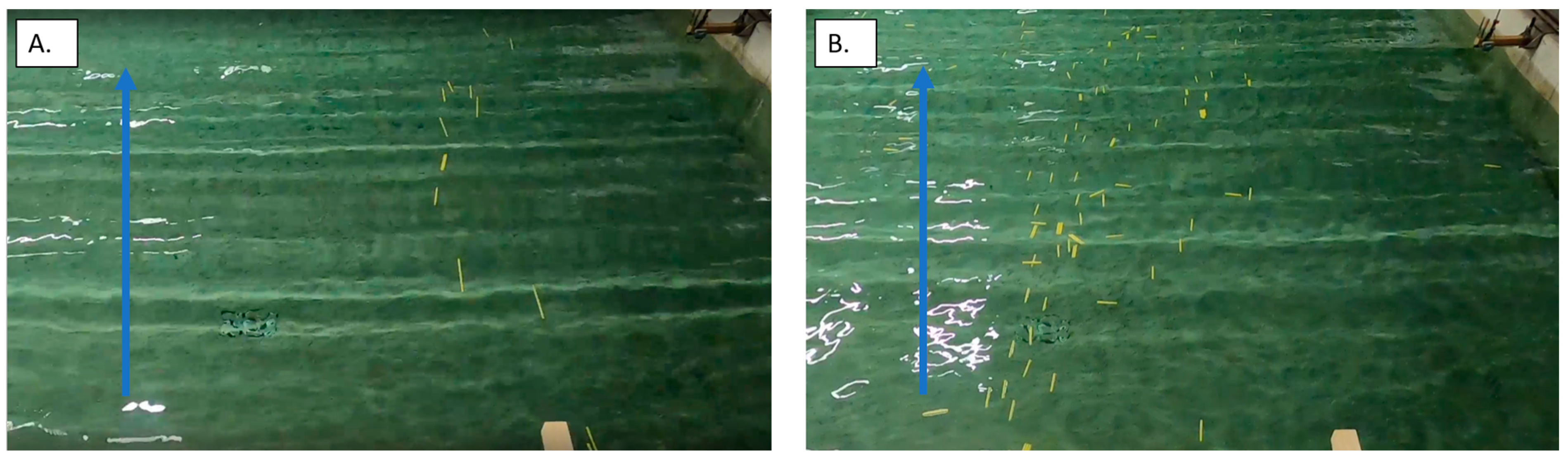
4.3. Size, Shape and Orientation of Objects

With regard to the size of the object, we can see that the experiments with plastic straws in Figure 8 give key information on this. The straws used in each experiment were the same plastic and concentration, the only changes were the size of the objects and, subsequently, the number of items used to create the concentration (i.e., as the size of straws halved, the number of objects doubled). We can see that for the X-band frequency, a significant difference in backscattering was found when the straws were 24 cm and 12 cm. However, when the straws were 6 cm, we found no significant difference. This can possibly be related to the wavelength of the X-band frequency being similar to the size of the object and causing difficulties, but it may also be due to the orientation of the objects travelling through the water. It should be noted that when the full-length straws were placed into the water, they travelled nearly exclusively perpendicular to the waves. However, when the size was reduced to 6 cm, the orientation of the straws changed as some moved perpendicular with the wave and others moved parallel, while some moved diagonally (as seen in Figure 8). We believe that this orientation will have an effect on the backscattering, potentially due to the size of the object front that is facing the radar changing, or with changes in the polarisation. However, due to the lack of quad-polarimetric X-band data, an investigation into these effects was not possible.

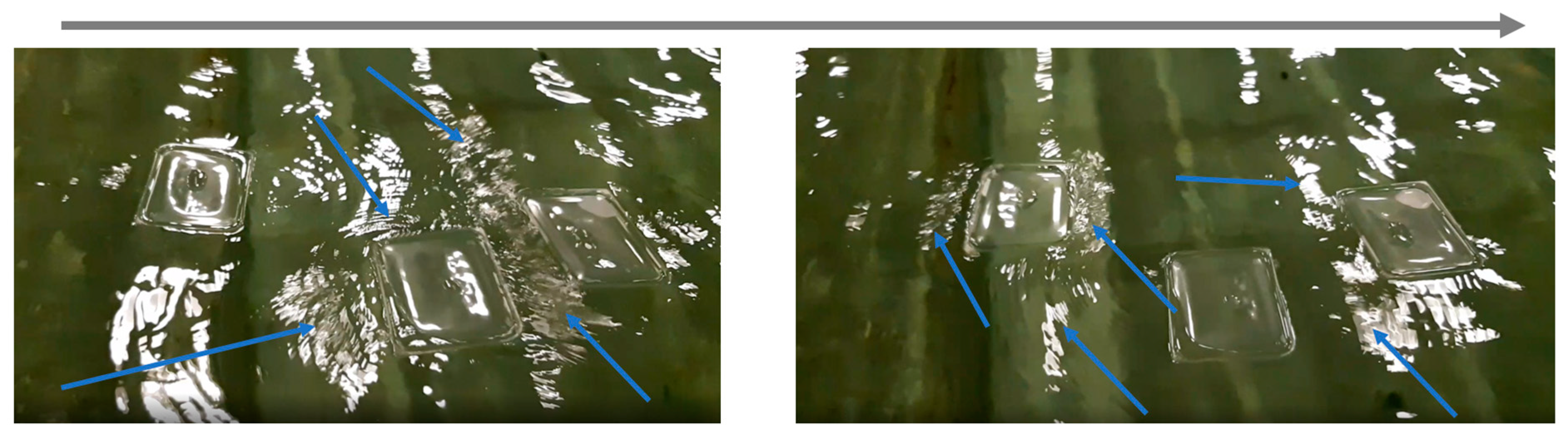
An interesting observation from the measurement campaigns was that some of the flat objects, such as the lids, had strong backscattering. The scattering mechanism that may be dominant here is the wave generation scattering from the object, due to the impinging of waves. We noted that capillary wave generation in flatter objects was especially pronounced (as seen in Figure 9).

Another interesting observation in relation to our scattering mechanism concept is that a significant difference in backscatter was found in the X-band measurements of plastic bottles (both 20 g and 40 g/m²). Interestingly, when these bottles were filled with water and became partially submerged, this significant difference in backscatter could not be found anymore. We believe this helps strengthen the ‘indentation’ scattering hypothesis, as the water that is filling the space in the bottle is also filling in the indentation that would have been created from the ‘empty’ space inside the plastic. An example of this hypothesis is shown in Figure 10.

4.4. “Stripe” Features in Radargrams

In several radargrams we could observe “vertical stripes” of bright targets. We hypothesize that these are due to either breaking waves or particularly large waves moving along the tank. When a larger wave moves in the tank, it may produce conditions close to breaking where it generates capillary waves from the crest of the wave. Those waves are quite fast moving and, therefore, they smear their energy over all of the spectrum of the SFCW. This could be seen as, while the radar is doing the sweeping, they appeared in different range locations producing the smearing we observed as an almost vertical feature.

Those features were more visible at higher wave heights. Additionally, the tendency to break (and produce capillary waves) was stimulated by the presence of plastic, which presents discontinuities. Those capillary waves were the ones we identified as the third scattering mechanism, which during this phenomenon (of breaking waves) became the dominant one.

4.5. Wave Size

The size of the waves within the wave tank also dictated the radar capabilities for monitoring plastic. In most cases, 17 cm wave heights made the detection of plastic materials more difficult. We believe that this is due to the 17 cm waves breaking more and causing an increased roughness from the harsher waves, which masks any of the backscattering from the plastic materials. The exceptions to this are plastic lids and sheet materials, both of which are flat objects which created strong capillary wave interactions with the surrounding waves when moving through the wave tank. The increased wave height resulted in generating more capillary waves, which, therefore, facilitated detection even in this scenario.

4.6. Wind Conditions

In the open ocean, it was common to find changing wave conditions induced by changing wind speeds. Gusts of wind within the open ocean can generate foam and high frequency capillary waves. In some of our testing (marked irregular + capillary in tables above), we induced wind-driven capillary waves through the use of a fan located to the side of the wave tank. The fan was operational during both the reference and test acquisitions. We can see from Table 5 and Table 7 that plastic sheet materials at 8.3 g/m² were detectable in 9 cm irregular waves when the wind-induced capillary waves were not present. However, in our irregular + induced capillary wave testing, we found that the plastic sheet material became undetectable. This could be due to our ‘wave generation’ scattering mechanism being masked by the winds. These mechanisms need to be taken into account for future testing or missions.

4.7. Checking Stability

To ensure that the differences in backscattering were not caused by changes in the wave spectra generated by the wave generator over the measurement periods of each experiment, we tested a full test measurement of only waves (no plastic) against a reference measurement taken beforehand for each wave type used throughout the campaign. As seen in Table 6 and Table 7, we can observe that the full 5 cm, 9 cm, and 17 cm wave tests found no significant difference between the reference and test measurements from these experiments. This means that we can safely presume that the significant differences in backscattering were created from the addition of plastic into the tank and not from changes in the waves themselves over the measurement periods.

4.8. Extrapolation to Satellite Data

The use of C-band radar has previously been utilised in research to try and understand the capabilities of detection from space using Synthetic Aperture Radar (SAR). Topouzelis et al., 2019 [11] attempted to use Sentinel-1 (5.405 GHz) SAR imagery to monitor and detect plastic litter targets off the coast of Lesvos Island, Greece. They found a difference in backscatter where variations were found between a 10 × 10 m target made from plastic bottles and the surrounding water. However, there were no differences found between two other targets of the same size, made from plastic bags and from fishing nets. These observations were noticeable in the VV polarised Sentinel-1 imagery. Unfortunately, no X-band imagery was obtained during this study to compare the performance of different frequencies. However, we can see that the use of C-band still has the potential to detect plastics in larger concentrations and accumulations.

The use of Sentinel-1 C-band SAR data has also been used to monitor large plastic accumulations by dams. Simpson et al., 2022 [21] found that large accumulations of primarily plastic materials were detectable using Sentinel-1 SAR data. Using change detection algorithms, they found the best detector, the Optimisation of Power Difference detector, could detect plastic accumulations with accuracies varying from 85 to 95%, depending on the false alarm rate within their test cases. This further showcases the use of C-band radar imaging for the remote sensing of plastic accumulations.

We have seen that X-band appears to be the most suitable frequency for detecting plastic pollution, compared with C-band, and that future missions (airborne or satellite) focusing on the detection of plastic pollution should focus on the use of this frequency. We believe that these results should aid future testing/experiments for plastic detection with radar and that the details within Section 4.1, Section 4.2, Section 4.3, Section 4.4, Section 4.5 and Section 4.6 can be used for future mission planning to tackle marine plastic pollution. Another point of note is that our range resolution from the ground-radar is 15 cm, which is a much finer resolution than most SAR satellites. However, new SAR X-band resolutions are capable of reaching a 25 cm resolution, as shown by the ICEYE constellation, and finer resolutions may be possible in the future.

To conclude, it has been shown that plastic can induce a difference in backscattering in the VV polarisation channel (mostly in X-band). It is, therefore, expected that a future plastic detector with satellite data will need to be built as an anomaly detector.

5. Future Work

This study has begun to shed light on radars’ capabilities in monitoring marine plastic litter from a lab-based setting. However, more wave heights, concentrations, and the use of real mixed targets could be used in future experiments. While this list of different test conditions is not exhaustive, we have started testing a set of conditions that cover calm to mid sea states.

A possible next stop of research would involve scaling this upward, with radar measurements being taken from on-board an airplane. This will allow us to see the scalability of this experiment into the real world and to begin to quantify if these techniques would be possible from space in the future.

6. Conclusions

The practice of remote sensing in the detection of marine litter debris on water is a relatively new field and the potential and capabilities of radar is yet to be fully understood. This study has shown that backscattering differences in C- and X-band between the reference ‘clean’ water and test water filled with plastic can be detected in some conditions (based on the statistical analysis). Overall, the results indicated that the X-band frequency performed significantly better than the C-band frequency in detecting differences in backscattering when plastic materials were within the water, with X-band detecting significant differences in backscattering in 37/60 cases compared with C-band detecting differences in 10/60 cases. We also found that the difference in backscattering was dependent on the size and shape of the plastic object, as well as the wave conditions which the plastic is moving on. This article provides key information on the capabilities of radar for detecting marine plastic litter and provides details which can be used for future planning in regard to tackling the remote sensing of marine plastic pollution.