Abstract
Using airborne drones to monitor water quality in inland, transitional or coastal surface waters is an emerging research field. Airborne drones can fly under clouds at preferred times, capturing data at cm resolution, filling a significant gap between existing in situ, airborne and satellite remote sensing capabilities. Suitable drones and lightweight cameras are readily available on the market, whereas deriving water quality products from the captured image is not straightforward; vignetting effects, georeferencing, the dynamic nature and high light absorption efficiency of water, sun glint and sky glint effects require careful data processing. This paper presents the data processing workflow behind MapEO water, an end-to-end cloud-based solution that deals with the complexities of observing water surfaces and retrieves water-leaving reflectance and water quality products like turbidity and chlorophyll-a (Chl-a) concentration. MapEO water supports common camera types and performs a geometric and radiometric correction and subsequent conversion to reflectance and water quality products. This study shows validation results of water-leaving reflectance, turbidity and Chl-a maps derived using DJI Phantom 4 pro and MicaSense cameras for several lakes across Europe. Coefficients of determination values of 0.71 and 0.93 are obtained for turbidity and Chl-a, respectively. We conclude that airborne drone data has major potential to be embedded in operational monitoring programmes and can form useful links between satellite and in situ observations.
1. Introduction
Unmanned aerial vehicles (UAVs), more commonly referred to as drones, carrying optical sensors, are already embedded in various land mapping and monitoring applications. Drones are easy-to-use, flexible in deployment and can be flown at low altitudes, even in the presence of clouds. Some airborne drones have been developed to collect in situ water samples which can be further analysed in the lab, e.g., [1,2,3]. In contrast to the water-sampling drones, drones with camera systems have the advantage of providing near-real-time information at a high spatial resolution, making it possible to observe small-scale variations in optically active water constituents and in nearshore and shoreline zones where satellites suffer from mixed pixels and adjacency effects [4]. Two major types of drone platforms exist: (i) fixed-wing drones typically have long endurance but are relatively expensive and need a runaway for take-off; (ii) multi-copter platforms are relatively cheap and only need a vertical take-off and landing spot. Vertical Take-Off and Landing (VTOL) systems are between fixed-wing drones with vertical take-off and landing capabilities, eliminating the need for a runway. For most studies in mapping surface water resources using drones (77%), the multi-copter system is preferred because of the lower cost and small take-off location [5]. Various cameras can be mounted under drones, ranging from broadband Red–Green–Blue (RGB) images to multi- and hyperspectral sensors. The type of application defines the preferred camera system, with RGB the cheapest but often lacking sufficient spectral information for water-quality applications.
Since 2013, interest in using drone data for optical water quality retrieval is steadily increasing [5], with several publications focussing on turbidity, chlorophyll-a (Chl-a) concentrations and macrophytes, e.g., [6,7,8,9], in lakes, ponds, rivers and reservoirs. Most of these studies include generic processing software and tools to convert the collected raw digital number data into reflectance values. Addressing drones to monitor optical water properties is a bit more challenging compared to land-based monitoring. In contrast to land applications, drone imagery collected over water bodies rarely includes non-moving stationary points. The presence of stationary points allows the use of standard (stereo) photogrammetry methods like Structure-from-Motion (SfM) [10]. Through triangulation based on subsequent images with sufficient overlap, the 3D coordinates of points are determined. The accuracy of the position and motion sensor is not crucial for the quality of the photogrammetry output. However, in the absence of stationary points, this technique is not applicable.
Another difference compared to land is that water acts as a mirror. The signal detected by the sensor is thus influenced by surface specular reflection from the sun and/or sky glint. The authors of [11] investigated four different methods to correct for surface reflected light, including Hydrolight simulations [12], the dark pixel assumption (NIR = 0), a baseline function or a “deglinting” approach. More recently, drone-based atmospheric correction tools are becoming available, like DROACOR [13]. This fully automatic physics-based processor uses pre-calculated look-up tables generated with libRadtran radiative transfer code to correct for atmospheric conditions.
While drone observations are very useful in local monitoring studies, they also have the potential to be used in satellite validation efforts. As pointed out by [14], the validation of satellite products requires high-quality in situ measurements, referred to as Fiducial Reference Measurements (FRM). Before a measurement can be labelled as FRM, it should (i) be accompanied by an uncertainty budget for all instruments, derived measurement and validation methods, (ii) adhere to openly available measurement protocols and community-wide management practices, (iii) have documented evidence of International System of Units (SI) traceability and (iv) be independent of the satellite retrieval process [15].
In this study, we present the workflow behind MapEO water: a sensor-independent cloud-based drone solution that provides georeferenced water-leaving reflectance and water quality parameters. MapEO water uses direct georeferencing [16], a technique that works in the absence of stationary points, and iCOR4Drones. This module corrects for glint effects under different cloud conditions using MODTRAN5 [17] based look-up tables (LUT). A validation of MapEO water is performed for DJI Phantom 4pro (DJI PH4) RGB and MicaSense multispectral data in various field campaigns across Europe. Simultaneous with the drone flights, in situ reflectance and water quality parameters were collected for validation. In addition, a comparison between satellite, drone and in situ data is conducted for the North Sea in Belgium.
2. Materials and Methods
2.1. MapEO Water Workflow
The VITO MapEO water (https://remotesensing.vito.be/case/mapeo-water, accessed on 1 January 2023) workflow allows the operational processing of drone data in a cloud environment. Once the drone pilot uploads the data into the cloud environment [18], the processing workflow can be initiated. This workflow comprises five steps: (i) georeferencing, which allows the projection of drone imagery; (ii) radiometric correction to convert raw digital numbers into radiance; (iii) conversion from radiance to water-leaving reflectance; (iv) conversion of water-leaving reflectance into optical water quality products like turbidity, suspended sediments or Chl-a concentrations. Each step is detailed below.
2.1.1. Georeferencing
Georeferencing is performed using a technique called direct georeferencing [16], i.e., making direct use of the information provided by the position and motion sensor mounted on the drone platform for georeferencing. The surface to project on is assumed to be flat, and its elevation only depends on the user-specified height difference between the water level and drone take-off location. The obtained accuracy in pixel position is mainly determined by the quality of the auxiliary sensors. The more accurate they are, the better the projection will be.
2.1.2. Radiometric Correction
The radiometric correction converts the raw digital numbers for each pixel of an image and each spectral band into absolute spectral radiance values with units of W m-2 sr−1 nm−1. The correction combines sensor black level correction, the sensitivity of the sensor, sensor gain and exposure settings and lens vignette effects. The formula for radiometric correction of drone data, following [19]:
with
- the spectral radiance measured by the camera and expressed in W/m2/sr/nm;
- vignette model to correct for the fall-off in light sensitivity that occurs in pixels further from the centre of the image;
- are radiometric calibration coefficients;
- the sensor gain setting;
- the normalised raw pixel value, i.e., the raw digital number of the pixel divided by the number of bits in the image (4096 for a 12-bit and 65536 for a 16-bit image);
- the normalised black level value;
- the image exposure time;
- the pixel column and row number.
Some camera systems like MicaSense store all required information in the metadata of the camera-generated image files. Other camera systems, like the DJI PH4pro, lack radiometric calibration coefficients, simplifying Equation (1) to
with
- the pseudo radiance received by the sensor;
- an empirically defined vignetting model, by normalising all pixels of a homogenous surface and storing the defined ratios which lower towards the edges of the image;
- is the camera f-number, i.e., the ratio of the camera’s focal length to the aperture.
2.1.3. Conversion from Radiance to Water-Leaving Reflectance
To derive the water-leaving reflectance (), irradiance () and sky glint () should be corrected. Water-leaving reflectance is the ratio of water-leaving radiance and water surface downward irradiance and reflects information on the substances in the upper layer of the water body [20]. The sensor captures not only water-leaving radiance but also specular reflection of the sun and sky at the water surface, referred to as sun glint and sky glint, respectively. The influence of sun glint can be reduced through thoughtful flight planning [18], but sky glint remains an important contributor. In accordance with [21] can be retrieved as follows:
with
- the wavelength;
- the Fresnel reflectance;
- the view zenith angle;
- the view azimuth angle;
- the downwelling sky radiance;
- the downwelling irradiance above the surface;
- the surface reflectance;
- referred to as sky glint.
There are two ways to calculate the surface reflectance: (i) using spectral reference panels in the field or (ii) making use of a downwelling light sensor (DLS).
When using spectral reference panels, i.e., panels that have a known reflectance, the equation can be written as
where stands for the known spectral reflectance of the spectral reference panels at wavelength , and the radiance of the spectral panels in field measured by the camera.
If a DLS is available, the irradiance coming from the sky is measured directly in units (W/m2/nm). When the DLS is placed parallel with the ground surface, can be calculated by dividing with the irradiance measured by the DLS ( and multiplied with :
However, the DLS will often not be placed parallel with the ground, and a correction for sensor and illumination angles is required. In addition, a Fresnel correction to correct for the air–sensor interface is needed. As described in [19], the Equation can be rewritten into
with
- percentage diffuse irradiance;
- Fresnel coefficient for air-sensor interface;
- solar-sensor angle, i.e., the angle between the DLS vector and sun vector;
- sun elevation angle.
The remaining unknown term in Equation (3) is the sky glint. This component can be derived using the iCOR4Drones tool, an adapted version of iCOR [22] for drone imagery. The tool relies on the MODTRAN5 [14] look-up tables (LUT) as described in [23]. Required input parameters are:
- Sun zenith angle;
- View zenith angles;
- Relative azimuth angle;
- Cloud type: Open Sky, Cumulus, Stratus, Altostratus;
- Spectral Response curves of the camera.
This approach assumes that the pixel is not affected by direct sun glint (realised by avoiding sun glint as part of flight planning) and that wind speed is sufficiently low to avoid foam or white cap radiance. Remaining effects of sun glint and/or foam can still be masked in output products. Light is considered to be unpolarised, and the sky radiance is distributed in a uniform way. If and are known, the water-leaving reflectance can be calculated (Equation (3)).
2.1.4. Conversion from Water-Leaving Reflectance to Water Quality Products
Once is calculated, other water quality products, like turbidity, Chl-a or suspended sediment concentrations, can be derived. In this work, we use the algorithm as described by [24] to derive turbidity and either OC3 [25] or Gilerson [26] algorithms to calculate Chl-a concentrations. Turbidity is estimated as
with the water-leaving reflectance for a given waveband, and and two wavelength dependent calibration coefficients ( = 366.14, = 0.1956 when using the Red band).
Chl-a for clear water types with low turbidity is derived as follows:
with
- and calibration coefficients ().
In relatively turbid waters, Chl-a is instead derived following
2.2. Validation in Inland and Coastal Waters
2.2.1. Study Sites
Field campaigns were organised at different locations across Europe:
- -
- Lake Balaton in Hungary is the largest lake in Europe, with an area of 592 km2. Despite its large surface area, it is very shallow, with a mean depth of approximately 3.2 m. The trophic state of Lake Balaton varies between mesotrophic and eutrophic regimes. In addition, Kiss Balaton varied in trophic status and suspended matter concentration.
- -
- The Belgian North Sea covers an area of about 3454 km2. It is a sensitive ecosystem under considerable pressure from intensive human activity such as sand and gravel extraction, dumping of dredged material, wind farming, fishing, shipping and tourism. The coastal area is subject to anthropogenic eutrophication from land-based nutrients rinsing in rivers and flowing into the sea [27].
- -
- Razelm-Sinoe Lagoon is a coastal lagoon system attached to the southern part of the Danube Delta, located on the Romanian shoreline of the Black Sea. The lagoon system has been impacted by anthropogenic interventions (e.g., closing the connection with the sea), affecting its natural evolution [28]. The inflow of nutrient-rich Ranuve waters has increased eutrophication in the lagoon, especially in the last 20 years [29].
- -
- Rupelmondse Creek is a ground- and rainwater-fed waterbody connected to the Scheldt river through leaking non-return valves. The Scheldt water differs from the creek water in suspended sediments and Chl-a concentration. Knowledge about the extent of the inflow plume (including short- and long-term temporal variation) is necessary for ecologically sound water management in the polder.
- -
- Lake Marathon is a water supply reservoir located in Greece. It has a total surface area of about 2.4 km2 and maximum depth of 54 m. The reservoir is constructed from concrete and operates as a backup source for the water supply system of the greater Attica region and as a primary regulating reservoir. Seasonal algae fluctuations and prevention of pollution caused by trespassing and agricultural activities require careful monitoring of the lake [30].
Figure 1 shows the geographic locations of the field campaigns.
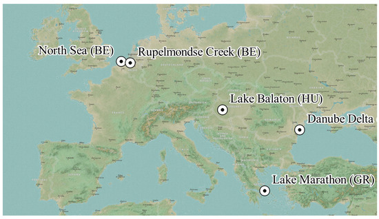
Figure 1.
Drone flights performed across Europe for which simultaneous in situ data were collected.
2.2.2. Drone Data
Drone flights were performed with the standard RGB camera under a DJI Phantom 4 Pro (DJI PH4), the multispectral MicaSense RedEdge-M (MSREM) or the MicaSense Dual camera (MSDual), consisting of an MSREM and a MicaSense RedEdge-M Blue camera (MSBLUE). Table 1 summarises the technical characteristics of the used camera systems, while Figure 2 shows the spectral characteristics. The spectral characteristics of the PH4pro and MS-REM were measured in the NERC Field Spectroscopy Facility (FSF) (UK) according to the methodology described by [31]. For the MS-BLUE, a Gaussian spectral response was assumed around the central wavelength and taking into account the full width at half maximum (FWHM). Flight protocols, as described in [18], were followed to reduce the pixels affected by sun glint. The most important considerations were (i) to mount the camera under a pitch angle of ±8° from nadir where possible; (ii) during flight, point the camera in the opposite direction to the sun to avoid the majority of sun glint effects; (iii) store data in raw digital number format; (iv) obtain information of the irradiance either using a DLS or place spectrally calibrated Lambertian reference panels within the field of view of the camera, as explained in 2.1.1; (v) estimate or measure the relative height difference between the take-off location of the drone and the water level. This last point is important to the relative height difference between the drone and the water level.

Table 1.
Summary of three different camera systems used in this study.
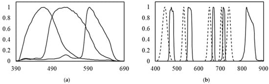
Figure 2.
Spectral response curves showing the normalised response as a function of wavelength [27] for (a) DJI PH4pro and (b) MS-DUAL, consisting of MS-REM (solid lines) and MS-BLUE (striped lines).
The drone data were processed with MapEO water, as discussed in Section 2.1. For validation of the water-leaving reflectance and water quality products, additional quality checks were performed. Two rules were applied as quality control to exclude non-water pixels like reflectance coming from vessels or shadow:
- -
- ρw –665 > ρw – 865;
- -
- min(ρw) > −0.05.
In addition, the lowest reflectance in the spectral range from 705 to 865 nm was subtracted from all wavebands. In low to median turbid waters, it can be assumed that the reflectance in the NIR bands is nearly zero, as water strongly absorbs in this spectral range [32]. Non-zero reflectance can be due to residual glint or insufficient correction of irradiance. This subtraction is further referred to as the RedEdge-NIR subtraction. The median value of a 1 × 1 m box around the in situ coordinate was calculated. As one in situ sampling location can fall within different images due to overlap, mean and standard deviations were derived for each in situ measurement. For visualisation, mosaics were generated in a post-processing step, which includes masking non-water pixels to avoid, e.g., pixels affected by vessels, down-sampling to a lower resolution and finally, mosaicking through calculation of mean and standard deviation of all pixels falling within a predefined “super-pixel”.
2.2.3. Match Up Data
Reflectance measurements were collected using the TriOS Ramses spectroradiometers, measuring 320–950 nm spectral range [33]. The remote-sensing reflectance, available online, was processed using the Fingerprint method [34], and only measurements passing the FingerPrint Pass Flag were retained in this study. The hyperspectral data were resampled to MS-REM, MS-BLUE and DJI PH4 pro bands using the spectral response functions provided in Figure 2 and multiplied with pi to obtain water-leaving reflectance.
Turbidity and Chl-a in situ values were measured using turbidity meters and HPLC or lab analysis, respectively. Samples and measurements were collected during the drone flights, limiting the maximum time difference to 45 min. All in situ measurements located within one pixel of 2 m of the drone mosaic were grouped, and mean and standard deviation values were calculated for this subset.
A Sentinel-2B MSI image acquired over the Belgian North Sea on 13 April 2021 was used and compared with drone and in situ observations. The Sentinel-2 tiles (31UDT, 31UDS, 31UES and 31UET) were processed using the Terrascope Water processing workflow [35,36]. Terrascope (https://terrascope.be/en, accessed on 24 February 2023) is the Belgian platform for Copernicus satellite data, products, and services. Terrascope uses the semi-empirical algorithm of Nechad [24] and a band-switching approach to allow the derivation of both high turbid and low turbid values. The turbidity products are masked using WorldCover [37] for land masking and IdePix for cloud/cloud shadow masking.
Table 2 provides an overview of the different field campaigns and the corresponding in situ and satellite data used in this study.
Table 2.
Overview of drone flights: date, location and sensor are listed, as well as the in situ measurements used for validation. (DJI PH4 = DJI Phantom 4 Pro, MSREM = MicaSense RedEdge-M, MSDUAL = MicaSense Dual camera).
2.2.4. Validation Metrics
For the validation of the drone-based reflectance and water quality products, a linear least square regression was performed between the set of drone values and the set of in situ measurements. Intercept and slope values are provided, and the coefficient of determination (R2) and Root Mean Square Error (RMSE) were derived to evaluate the regression model:
with the predicted value of y and the mean value of y.
3. Results
3.1. Validation of Drone-Based Reflectance and Water Quality Products
Figure 3 shows the mean water-leaving reflectance spectra and standard deviation of all matchups collected within one flight at Lake Balaton and one at Kiss Balaton. The upper figures show the spectra without RedEdge-NIR subtraction, while the lower plots show the spectra when the RedEdge-NIR subtraction is applied. While the results for Lake Balaton are very similar in both cases, the spectra of Kiss Balaton improved significantly after performing the RedEdge-NIR subtraction. Although the spectral shape was well retrieved, an offset of nearly 0.03 was observed before applying an additional subtraction. This offset was reduced to <0.01, assuming that the lowest reflectance observed in the RedEdge-NIR spectral range should be zero.
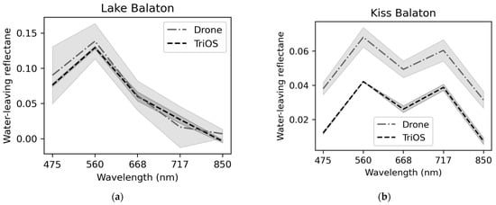
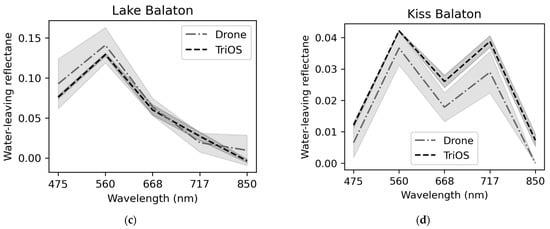
Figure 3.
Mean Water-Leaving Reflectance of Drone (grey) and TriOS Ramses (black) data plotted for two different flights at Lake Balaton (Lake Balaton and Kiss Balaton). The upper plots (a,b) show the reflectance without RedEdge-NIR subtraction. The lower plots (c,d) show the reflectance with RedEdge-NIR subtraction.
Figure 4 shows the water-leaving reflectance scatterplots (MSREM vs. TriOS) for the four spectral bands of the MSREM camera in Lake Balaton and Kiss Balaton. The NIR band is not included as this band was, in most cases, used for subtraction. All bands have a very low intercept value of < 0.005. The regression statistics of the Blue (475 nm), Green (560 nm) and Red (660 nm) bands yield an R2 > 0.93 and RMSE of 0.01. The slope for the Green band is nearly perfect (1.03), slightly too steep for the Blue band (1.21), and slightly too gentle for the Red band (0.88). The RedEdge band (717 nm) has an R2 value of 0.85 and a slope of 0.7. In addition, here, an intercept < 0.01 was noted, and an RMSE of 0.01.
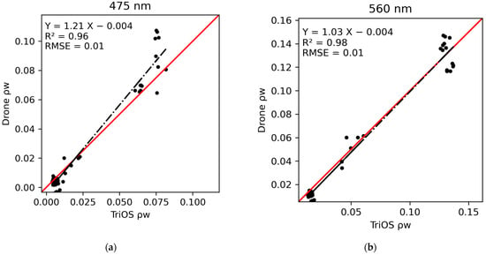
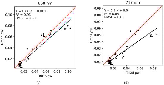
Figure 4.
Scatterplots of MS-REM versus in situ (TriOS) measured water-leaving reflectance in Lake Balaton. (a) Blue band (475 nm); (b) Green band (560 nm); (c) Red band (668 nm); and (d) Red Edge band (717 nm). Red line = 1:1 line, black line = regression line.
Figure 5 shows the scatter plots of turbidity, and Chl-a derived through MapEO water compared with in situ measurements. While turbidity results are retrieved from DJI PH4, and MSREM sensors, fewer results are available for Chl-a analysis as only flights conducted with MSDUAL cameras are suitable to derive this parameter. The turbidity trendline shows an offset of −2.47, slope of 1.08, R2 value of 0.71 and RMSE of 10.13. These statistics are based on values derived from the DJI PH4, and MSREM combined. Table 3 shows the turbidity results for each camera sensor separately and when combined. The DJI PH4 follows almost perfectly the 1:1 line with a low intercept. However, the scatter around this line is larger, with an RMSE of 14.35 and R2 value of 0.58. The MSREM has a slightly steeper slope (1.14) and offset of −4.53; the R2 and RMSE values are better, with values of 0.85 and 5.61, respectively. Chl-a values could only be retrieved using the MSDUAL camera. A slope of 1.12, an intercept of 2.491, an R2 of 0.93 and an RMSE of 9.34 was derived.
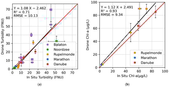
Figure 5.
Scatterplot of drone-derived versus in situ measured observations. (a) turbidity plot (circles are derived from MSREM, squares are derived from DJI PH4), (b) Chl-a plot (derived from MSDUAL). Red line = 1:1 line, black line = regression line.
Table 3.
Regression statistics of turbidity products when DJI PH4 and MSREM are combined and for both sensors separate.
Figure 6 and Figure 7 show examples of derived turbidity and Chl-a maps generated with MapEO water for Rupelmondse Creek, Lake Marathon and the Danube Delta. The Rupelmondse Creek shows low turbidity and high Chl-a values on the northern side, while the opposite is observed in the southern part. These observations are in line with expectations as the southern part is linked with the high turbid Scheldt River and consequently also subjected to tidal influences. The northern part is separated from the Scheldt through sluices. During extreme weather events (spring tides linked with the west of northwest storm wind), these sluices can be opened to avoid floodings at other locations along the Scheldt Estuary (part of SIGMA plan (https://sigmaplan.be/en/, accessed on 1 February 2023). The northern part is consequently hardly affected by tidal effects, and sediments in the water have sufficient time to settle. However, algae blooms can occur, resulting in increased Chl-a concentrations. Lake Marathon serves as a drinking water reservoir, affected from time to time by minor algae blooms. During the drone campaign, very low turbidity and Chl-a concentration were observed on the eastern part of the lake, which was in accordance with real-time field measurements from an unmanned surface vehicle (USV) operated by the Athens Water Supply and Sewage Company [38]. The example of the Danube Delta shows the impact of the Canalul Dunavat (Dunavat Canal) on Lacul Razelm (Lake Razelm): the highly turbid water supplied into the canal by the Danube, through its southern branch, Sfantu Gheorghe, flows into the lake, in a narrow plume. The concentrations of Chl-a in the inflow water are very low compared to the water of the lake. The lake is relatively shallow (0–3.5 m), and the algal blooms increase in intensity from spring to autumn. The plume of the canal and its extent into the lake is mainly controlled by wind, so most of the time, it remains very close to the inlet.
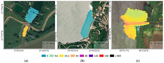
Figure 6.
Examples of generated mosaicked turbidity maps. A logarithmic colour scaling is applied with units expressed in FNU. (a) Rupelmondse Creek; (b) Lake Marathon; (c) Danube Delta.
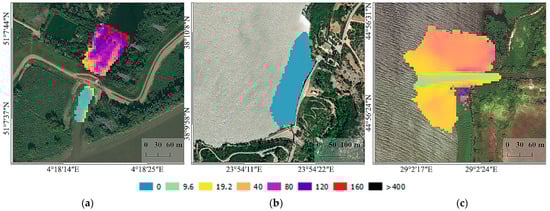
Figure 7.
Examples of generated mosaicked Chl-a maps. A logarithmic colour scaling is applied with units expressed in μg/L. (a) Rupelmondse Creek; (b) Lake Marathon; (c) Danube Delta.
3.2. Comparison of Satellite, Drone and In Situ Data
Figure 8 shows the Sentinel-2 derived turbidity product from 13 April 2021 10:59 UTC, obtained from Terrascope (see Section 2.2). The two locations of drone flights are marked in the figure. The drone flights were conducted with a DJI PH4pro drone. Location A was acquired at 10:05 UTC, and location B at 12:32 UTC. The DJI took off and landed on the Simon Stevin Research Vessel. Light fluctuations were corrected using a spectral reference panel onboard, as described in Section 2.1. Figure 9 shows two true colour drone images and the respective drone turbidity map, one for each location. The background colour represents the Sentinel-2 turbidity map. At location A, higher turbidity values were obtained from the drone data compared to the satellite data, while at location B both values are very comparable. Table 4 summarises the turbidity values derived from different sources: Sentinel-2, DJI PH4pro, and the in situ measured turbidity. The turbidity values of the drone data are in line with the in situ observations. For Sentinel-2, the values at location B are similar; for location A, almost half of the measured in situ and drone values were obtained. This can be caused by errors in the atmospheric correction or, as the drone data seems to support, high dynamics in a spatial and temporal context.
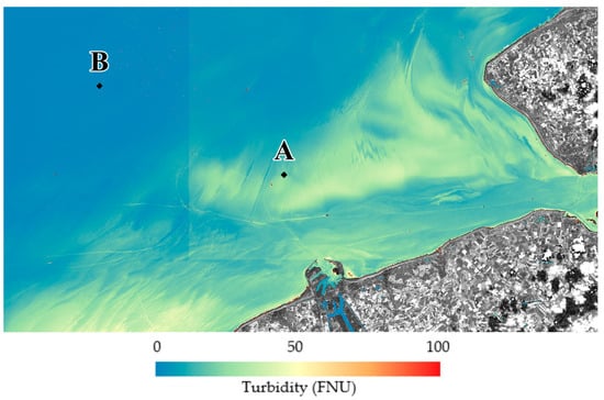
Figure 8.
Sentinel-2 derived turbidity product on 13 April 2021 at 10:59 UTC. The two locations of drone flights are marked with A and B.
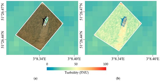
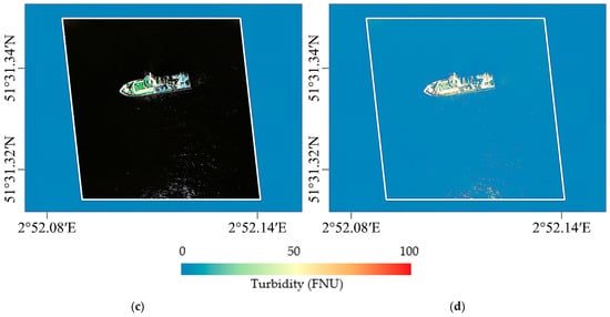
Figure 9.
True colour and turbidity products for the two locations. Sentinel-2-derived turbidity products serve as a background. (a) True colour drone image at location A, acquired at 10:05 UTC; (b) turbidity-derived product at location A; (c) True colour drone image at location B, acquired at 12:32 UTC; (d) turbidity-derived product at location B.
Table 4.
Turbidity values derived from Sentinel-2 MSI, DJI PH4pro and HACH in situ device for the two locations in the Belgian North Sea.
4. Discussion
4.1. Validation of Drone-Based Reflectance and Water Quality Products
The water-leaving reflectance, the base product of optical remote sensing over water and used to derive water quality parameters, shows a very good fit between in situ radiometric measurements performed from a ship and the observation from the drone platform using the MSREM camera (Figure 4). The water-leaving reflectance in the Blue, Green and Red bands has an R2 value of 0.93 and RMSE lower than 0.01. Their slopes vary between 0.86 and 1.22; the intercept is <0.005. Compared to these, the RedEdge band performs slightly less but is still reasonably good, with a slope of 0.7 and an R2 value of 0.85. These results were obtained after an additional correction by subtracting the lowest reflectance value in the 668–850 nm spectral range. This correction is often applied over surface waters, as water strongly absorbs in the NIR spectral range [32]. The offset can be caused by remaining glint effects, adjacency effects, or an insufficient correction for irradiance. As mentioned in Section 2.1, the irradiance is either derived from spectral reference panels placed in the field or from an irradiance sensor mounted vertically upwards on the drone platform. When the spectral reference panels are placed on the ground or a vessel, the signal of the panels, as detected by the camera sensor, can be affected by the surroundings (e.g., vegetation or vessel). In addition, rapidly changing cloud conditions make it challenging to use spectral reference panels, as the values retrieved at certain moments over the panels cannot be considered constant throughout the flight. Therefore, this additional subtraction using the lowest values in the 668–840 nm spectral range cannot be applied at all sites. Furthermore, as pointed out in [39], in extremely turbid waters, the assumption of a zero NIR reflectance is no longer valid. Therefore, caution should be taken on when and where to apply this correction.
The water quality products derived from water-leaving reflectance were validated with in situ measurements (Figure 5). Turbidity could be derived from both camera systems, the DJI PH4 and MSREM (also included in the MSDUAL set-up). When performing a regression analysis, it appeared that the DJI PH4 had good intercept and slope values (0.99 and 1.5, respectively) but low R2 (0.58) and RMSE values 14.35. For the MSREM, the slope and intercept were 1.14 and −4.53, while the R2 and RMSE were much better than the DJI PH4, with values of 0.85 and 5.61. These results indicate that it is possible to derive turbidity from a low-cost RGB sensor onboard a drone but with larger errors compared to multispectral data. Chl-a values can only be derived using the MSDUAL camera, limiting the number of match-ups. A slope of 1.12 and an intercept of 2.49 with R2 and RMSE of 0.93 and 9.34, respectively. These results illustrate the usefulness of drones for water quality monitoring. For turbidity, low-cost cameras can be used but at the cost of higher errors. For Chl-a, the sensor should have the correct wavelengths. This was the case for MSDUAL, but the MSBLUE sensor is no longer supported by MicaSense.
4.2. Comparison of Satellite, Drone and In Situ Data
In situ point observations are used to define, calibrate and validate algorithms and satellite-derived products. However, often the variability within a pixel is unknown when taking in situ measurements. In the example of the North Sea (Figure 9), a turbidity plume generated by the boat is still visible. However, the boat was located at a fixed position when taking the measurements. Radiometric measurements using an ASD FieldSpec spectroradiometer device were collected at the bow of the research vessel, using optimised viewing geometry with regard to the position of the sun. Water samples were collected at the starboard side of the vessel. Without the drone image, one would believe that both measurements, taken at nearly the same time and location, would represent the same water mass and condition. The drone image, however, shows a spatial heterogeneity in the colour of the water, which is amplified through the disturbance of the research vessel. Caution should thus be used when linking different measurements together. This example shows the importance of FRM for validation studies at multiple levels: drone validation efforts will benefit from in situ FRM data, while drone FRM data can become relevant for satellite validation studies. However, before drone data meet the FRM requirements, a full uncertainty budget should be performed. First, efforts are made for land-based camera applications [40].
4.3. Overall Considerations
Expectations about the areal coverage of a drone platform are often unrealistic. The octocopter drones used in this study have a limited endurance of about 30–45 min, resulting in a limited areal coverage of up to 10,000 m2. Besides flight time, the altitude and visual line of sight (VLOS) define the extent. Long-endurance drone systems are available on the market, which can fly tens of kilometres from the drone pilot at high altitudes. However, these systems are relatively expensive and require additional permissions to operate and local drone flight regulations might still limit operations. As pointed out by [3], in many countries, there are still stringent restrictions regarding where and how drones may be operated.
Working with drone data requires the capability to handle large volumes of data. With an image obtained every 3–5 s, up to 600 images can be easily obtained within one drone flight. In order to handle such large volumes of data, MapEO water is deployed in a cloud environment. Cloud-based processing has multiple advantages, including scalability, flexibility and data loss prevention. Final products can be reduced in size through mosaicking and compression. The MapEO water output product is accompanied by a GeoJSON metadata file [41] containing information on the unique identifier, bounding box, acquisition and processing date, drone platform and sensors, number of spectral bands and cloud conditions. Such a standardised approach is needed to manage large data volumes and catalogue results.
5. Conclusions
This paper presented the workflow behind MapEO water, a cloud-based data processing service that converts airborne drone data into georeferenced water quality products, like water-leaving reflectance, turbidity and Chl-a concentrations. Three different camera systems were tested: the DJI PH4pro containing only broad RGB spectral bands and the MS-REM and MS-DUAL with five and ten spectral bands in the VNIR, respectively. MapEO water contains four processing modules: (i) Georeferencing is conducted through direct georeferencing instead of structure-from-motion techniques common in land applications. These latter techniques are not applicable over water because of their dynamics; (ii) The radiometric correction converts raw digital numbers into radiance. The correction combines sensor black level correction, the sensitivity of the sensor, sensor gain and exposure settings, and lens vignette effects; (iii) conversion from radiance to water-leaving reflectance, taking sky glint effects into account through the iCOR4Drones module; (iv) in the final step, water-leaving reflectance is converted into turbidity and Chl-a water quality products.
Tests were performed at different lakes across Europe. Water-leaving reflectance was validated against TriOS measurements, whereas turbidity and Chl-a products were compared against turbidity meters and in situ water samples analysed in the laboratory. With an R2 of 0.71 and 0.93 and RMSE of 10.13 and 9.34 for turbidity and Chl-a, respectively, these results show the potential of using drone-based observations for water quality monitoring. In addition, airborne drone data can be used to connect satellites with in situ observations and are very helpful in understanding the spatial conditions when taking in situ measurements for calibration and validation of algorithms or regulatory monitoring.
Author Contributions
Conceptualisation, L.D.K. and R.M.; methodology, R.M. and L.D.K.; software, R.M. and D.D.M.; validation. R.M. and L.D.K.; formal analysis, L.D.K.; investigation, A.M.C., A.S., G.K., W.M., P.D.H., E.S. and A.T.; writing—original draft preparation, L.D.K.; writing—review and editing, R.M., E.K., S.S., I.R. and S.G.H.S.; visualization, L.D.K.; funding acquisition, I.R., E.K., S.S. amd S.G.H.S. All authors have read and agreed to the published version of the manuscript.
Funding
This research was funded by European Union’s Horizon 2020 research and innovation programme under grant agreement No 776480 (MONOCLE), grant agreement No 101004186 (Water-ForCE), and was supported by the Belgian Science Policy (Belspo) under Grant SR/00/381 (TIMBERS) and Grant SR/67/311 (DRONESED).
Data Availability Statement
Publicly available datasets were analysed in this study. This data can be found using the Web Coverage Service (WCS) service: https://mapeo.be/geoserver/MONOCLE/wcs, accessed on 1 February 2023. Credentials: monocle/monocle.
Acknowledgments
The authors wish to thank the NERC Field Spectroscopy Facility for making their infrastructure available for data calibration. Both the DJI PH4pro and MS-REM cameras were spectrally calibrated in their lab.
Conflicts of Interest
The authors declare no conflict of interest.
References
- Koparan, C.; Koc, A.B.; Privette, C.V.; Sawyer, C.B. In Situ Water Quality Measurements Using an Unmanned Aerial Vehicle (UAV) System. Water 2018, 10, 264. [Google Scholar] [CrossRef]
- Rodrigues, P.; Marques, F.; Pinto, E.; Pombeiro, R.; Lourenço, A.; Mendonça, R.; Santana, P.; Barata, J. An open-source watertight unmanned aerial vehicle for water quality monitoring. In Proceedings of the Conference OCEANS 2015—MTS/IEEE, Washington, DC, USA, 19–22 October 2015; pp. 1–6. [Google Scholar]
- Ryu, J.H. UAS-based real-time water quality monitoring, sampling, and visualization platform (UASWQP). HardwareX 2022, 11, e00277. [Google Scholar] [CrossRef] [PubMed]
- El Serafy, G.; Schaeffer, B.; Neely, M.-B.; Spinosa, A.; Odermatt, D.; Weathers, K.; Baracchini, T.; Bouffard, D.; Carvalho, L.; Conmy, R.; et al. Integrating Inland and Coastal Water Quality Data for Actionable Knowledge. Remote. Sens. 2021, 13, 2899. [Google Scholar] [CrossRef] [PubMed]
- Sibanda, M.; Mutanga, O.; Chimonyo, V.G.P.; Clulow, A.D.; Shoko, C.; Mazvimavi, D.; Dube, T.; Mabhaudhi, T. Application of Drone Technologies in Surface Water Resources Monitoring and Assessment: A Systematic Review of Progress, Challenges, and Opportunities in the Global South. Drones 2021, 5, 84. [Google Scholar] [CrossRef]
- Flynn, K.F.; Chapra, S. Remote Sensing of Submerged Aquatic Vegetation in a Shallow Non-Turbid River Using an Unmanned Aerial Vehicle. Remote. Sens. 2014, 6, 12815–12836. [Google Scholar] [CrossRef]
- Su, T.-C.; Chou, H.-T. Application of Multispectral Sensors Carried on Unmanned Aerial Vehicle (UAV) to Trophic State Mapping of Small Reservoirs: A Case Study of Tain-Pu Reservoir in Kinmen, Taiwan. Remote Sens. 2015, 7, 10078–10097. [Google Scholar] [CrossRef]
- Larson, M.D.; Milas, A.S.; Vincent, R.K.; Evans, J.E. Multi-depth suspended sediment estimation using high-resolution remote-sensing UAV in Maumee River, Ohio. Int. J. Remote. Sens. 2018, 39, 5472–5489. [Google Scholar] [CrossRef]
- De Keukelaere, L.; Moelans, R.; Strackx, G.; Knaeps, E.; Lemey, E. Mapping water quality with drones: Test case in Texel. Terra Et Aqua 2019, 157, 6–16. [Google Scholar]
- Westoby, M.; Brasington, J.; Glasser, N.F.; Hambrey, M.J.; Reynolds, J.M. ‘Structure-from-Motion’ photogrammetry: A low-cost, effective tool for geoscience applications. Geomorphology 2012, 179, 300–314. [Google Scholar] [CrossRef]
- Windle, A.E.; Silsbe, G.M. Evaluation of Unoccupied Aircraft System (UAS) Remote Sensing Retrievals for Water Quality Monitoring in Coastal Waters. Front. Environ. Sci. 2021, 9, 674247. [Google Scholar] [CrossRef]
- Mobley, C.D. Polarized reflectance and transmittance properties of windblown sea surfaces. Appl. Opt. 2015, 54, 4828–4849. [Google Scholar] [CrossRef]
- Schläpfer, D.; Popp, C.; Richter, R. Drone Data Atmospheric Correction Concept For Multi—And Hyperspectral Imagery—The Droacor Model. Int. Arch. Photogramm. Remote Sens. Spat. Inf. Sci. 2020, 43, 473–478. [Google Scholar] [CrossRef]
- Ruddick, K.G.; Voss, K.; Boss, E.; Castagna, A.; Frouin, R.; Gilerson, A.; Hieronymi, M.; Johnson, B.C.; Kuusk, J.; Lee, Z.; et al. A Review of Protocols for Fiducial Reference Measurements of Water-Leaving Radiance for Validation of Satellite Remote-Sensing Data over Water. Remote. Sens. 2019, 11, 2198. [Google Scholar] [CrossRef]
- Donlon, C.J.; Wimmer, W.; Robinson, I.; Fisher, G.; Ferlet, M.; Nightingale, T.; Bras, B. A Second-Generation Blackbody System for the Calibration and Verification of Seagoing Infrared Radiometers. J. Atmos. Ocean. Technol. 2014, 31, 1104–1127. [Google Scholar] [CrossRef]
- Mian, O.; Lutes, J.; Lipa, G.; Hutton, J.J.; Gavelle, E.; Borghini, S. Direct georeferencing on small unmanned aerial platforms for improved reliability and accuracy of mapping without the need for ground control points. ISPRS-Int. Arch. Photogramm. Remote. Sens. Spat. Inf. Sci. 2015, 397–402. [Google Scholar] [CrossRef]
- Berk, A.; Anderson, G.P.; Acharya, P.K.; Bernstein, L.S.; Muratov, L.; Lee, J.; Fox, M.; Adler-Golden, S.M.; Chetwynd, J.J.H.; Hoke, M.L.; et al. MODTRAN5: 2006 update. In Proceedings of the SPIE 6233, Algorithms and Technologies for Multispectral, Hyperspectral, and Ultraspectral Imagery XII, Orlando, FL, USA, 8 May 2006; Volume 6233, p. 62331F. [Google Scholar] [CrossRef]
- De, K.L.; Moelans, R.; De, M.D.; Strackx, G. RPAS—Remotely Piloted Aircraft Systems—Deployment and Operation Guide; Zenodo: Geneve, Switzerland, 2022. [Google Scholar] [CrossRef]
- MicaSense Inc. “Tutorial 3—DLS Sensor Basic Usage” Micasense/Imageprocessing GitHub. 2017–2019. Available online: https://micasense.github.io/imageprocessing/MicaSenseImageProcessingTutorial1.html (accessed on 20 September 2022).
- Gao, M.; Li, J.; Zhang, F.; Wang, S.; Xie, Y.; Yin, Z.; Zhang, B. Measurement of Water Leaving Reflectance Using a Digital Camera Based on Multiple Reflectance Reference Cards. Sensors 2020, 20, 6580. [Google Scholar] [CrossRef]
- Sterckx, S.; Knaeps, E.; Ruddick, K. Detection and correction of adjacency effects in hyperspectral airborne data of coastal and inland waters: The use of the near infrared similarity spectrum. Int. J. Remote. Sens. 2011, 32, 6479–6505. [Google Scholar] [CrossRef]
- De Keukelaere, L.; Sterckx, S.; Adriaensen, S.; Knaeps, E.; Reusen, I.; Giardino, C.; Bresciani, M.; Hunter, P.; Neil, C.; Van der Zande, D.; et al. Atmospheric correction of Landsat-8/OLI and Sentinel-2/MSI data using iCOR algorithm: Validation for coastal and inland waters. Eur. J. Remote. Sens. 2018, 51, 525–542. [Google Scholar] [CrossRef]
- Biesemans, J.; Sterckx, S.; Knaeps, E.; Vreys, K.; Adriaensen, S.; Hooyberghs, J.; Nieke, J.; Meuleman, K.; Kempeneers, P.; Deronde, B.; et al. Image processing workflows for airborne remote sensing. In Proceedings of the 5th EARSeL SIG Imaging Spectroscopy Workshop, Bruges, Belgium, 23–25 April 2007. [Google Scholar]
- Nechad, B.; Ruddick, K.G.; Neukermans, G. Calibration and validation of a generic multisensor algorithm for mapping of turbidity in coastal waters. In Proceedings of the SPIE—The International Society for Optical Engineering, Berlin, Germany, 9 September 2009; p. 7473. [Google Scholar]
- O’Reilly, J.E.; Maritorena, S.; Mitchell, B.G.; Siegel, D.A.; Carder, K.L.; Garver, S.A.; Kahru, M.; McClain, C. Ocean color chlorophyll algorithms for SeaWiFS. J. Geophys. Res. Earth Surf. 1998, 103, 24937–24953. [Google Scholar] [CrossRef]
- Gilerson, A.A.; Gitelson, A.A.; Zhou, J.; Gurlin, D.; Moses, W.; Ioannou, I.; Ahmed, S.A. Algorithms for remote estimation of chlorophyll-a in coastal and inland waters using red and near infrared bands. Opt. Express 2010, 18, 24109–24125. [Google Scholar] [CrossRef]
- Lancelot, C.; Rousseau, V.; Gypens, N. Ecologically based indicators for Phaeocystis disturbance in eutrophied Belgian coastal waters (Southern North Sea) based on field observations and ecological modelling. J. Sea Res. 2009, 61, 44–49. [Google Scholar] [CrossRef]
- Bretcan, P.; Murărescu, M.O.; Samoilă, E.; Popescu, O. The modification of the ecological conditions in the Razim-Sinoie lacustrine complex as an effect of the anthropic intervention. In Proceedings of the XXIVth Conference of the Danubian Countries, Bled, Slovenia, 2–4 June 2008; ISBN 978-961-91090-2-1. [Google Scholar]
- Stanica, A.; Scrieciu, A.; Bujini, J.; Teaca, A.; Begun, T.; Ungureanu, C. “Razelm Sinoie Lagoon System—Stat of the Lagoon Report,” in Deliverable 2.2. ARCH (Architecture and Roadmap to Manage Multiple Pressures on Lagoons) FP7 Project, EC Grant 282748. 2013; Unpublished Report. [Google Scholar]
- Katsouras, G.; Chalaris, M.; Tsalas, N.; Dosis, A.; Samios, S.; Lytras, E.; Papadopoulos, K.; Synodinou, A. Integrated ecosystem ecology (Chlorophyll-a) of EYDAP’s Reservoirs profiles by using robotic boats. In Proceedings of the 5th International Conference ‘Water Resources and Wetlands’, Tulcea, Romania, 8–12 September 2021; Available online: http://www.limnology.ro/wrw2020/proceedings/23_Katsouras.pdf (accessed on 9 September 2021), ISSN 2285-7923.
- Burggraaff, O.; Schmidt, N.; Zamorano, J.; Pauly, K.; Pascual, S.; Tapia, C.; Spyrakos, E.; Snik, F. Standardized spectral and radiometric calibration of consumer cameras. Opt. Express 2019, 27, 19075–19101. [Google Scholar] [CrossRef] [PubMed]
- Gordon, H.R.; Wang, M. Retrieval of water-leaving radiance and aerosol optical thickness over the oceans with SeaWiFS: A preliminary algorithm. Appl. Opt. 1994, 33, 443–452. [Google Scholar] [CrossRef] [PubMed]
- Hunter, P.; Riddick, C.; Werther, M.; Martinez Vicente, V.; Burggraaff, O.; Blake, M.; Spyrakos, E.; Tóth, V.; Kovács, A.; Tyler, A. In Situ Bio-Optical Data in Lake Balaton, MONOCLE H2020 Project (Version v1) [Data Set]; Zenodo: Geneve, Switzerland, 2021. [Google Scholar] [CrossRef]
- Simis, S.G.; Olsson, J. Unattended processing of shipborne hyperspectral reflectance measurements. Remote. Sens. Environ. 2013, 135, 202–212. [Google Scholar] [CrossRef]
- De Keukelaere, L.; Landuyt, L.; Knaeps, E. Terrascope Sentinel-2 Algorithm Theoretical Base Document (ATBD) S2–RHOW–V120. 2022. Available online: https://docs.terrascope.be/DataProducts/Sentinel-2/references/VITO_S2_ATBD_S2_RHOW_V120.pdf (accessed on 23 February 2023).
- De Keukelaere, L.; Landuyt, L.; Knaeps, E. Terrascope Sentinel-2 Algorithm Theoretical Base Document (ATBD) S2–Water Quality–V120. 2022. Available online: https://docs.terrascope.be/DataProducts/Sentinel-2/references/VITO_S2_ATBD_S2_WATER_QUALITY_V120.pdf (accessed on 23 February 2023).
- Zanaga, D.; Van De Kerchove, R.; De Keersmaecker, W.; Souverijns, N.; Brockmann, C.; Quast, R.; Wevers, J.; Grosu, A.; Paccini, A.; Vergnaud, S.; et al. ESA WorldCover 10 m 2020 v100; Zenodo: Geneve, Switzerland, 2021. [Google Scholar] [CrossRef]
- Katsouras, G.; Konstantinopoulos, S.; De Keukelaere, L.; Moelans, R.; Christodoulou, C.; Bauer, P.; Tsalas, N.; Hatzikonstantinou, P.; Lioumbas, I.; Katsiapi, M.; et al. Unmanned Vehicles combined with satellite observations as a complement tool for water quality of Lake Marathon. In Proceedings of the EuroGEO Workshop 2022, Athens, Greece, 7–9 December 2022; Available online: http://intcatch.eu/images/Katsouras_poster_EuroGEO2022_v1.pdf (accessed on 23 February 2023).
- Knaeps, E.; Doxaran, D.; Dogliotti, A.; Nechad, B.; Ruddick, K.; Raymaekers, D.; Sterckx, S. The SeaSWIR dataset. Earth Syst. Sci. Data 2018, 10, 1439–1449. [Google Scholar] [CrossRef]
- Brown, L.A.; Camacho, F.; García-Santos, V.; Origo, N.; Fuster, B.; Morris, H.; Pastor-Guzman, J.; Sánchez-Zapero, J.; Morrone, R.; Ryder, J.; et al. Fiducial Reference Measurements for Vegetation Bio-Geophysical Variables: An End-to-End Uncertainty Evaluation Framework. Remote. Sens. 2021, 13, 3194. [Google Scholar] [CrossRef]
- Butler, H.; Daly, M.; Doyle, A.; Gillies, S.; Hagen, S.; Schaub, T.; The GeoJSON Format. Internet Standards Track document. 2016. Available online: https://www.rfc-editor.org/rfc/rfc7946 (accessed on 23 February 2023).
Disclaimer/Publisher’s Note: The statements, opinions and data contained in all publications are solely those of the individual author(s) and contributor(s) and not of MDPI and/or the editor(s). MDPI and/or the editor(s) disclaim responsibility for any injury to people or property resulting from any ideas, methods, instructions or products referred to in the content. |
© 2023 by the authors. Licensee MDPI, Basel, Switzerland. This article is an open access article distributed under the terms and conditions of the Creative Commons Attribution (CC BY) license (https://creativecommons.org/licenses/by/4.0/).