Article

Spectral Mixing Theory-Based Double-Branch Network for Spectral Super-Resolution

1
Aerospace Information Research Institute (AIR), Chinese Academy of Sciences (CAS), Beijing 100094, China
2
University of Chinese Academy of Sciences (UCAS), Beijing 100049, China
*
Author to whom correspondence should be addressed.
Remote Sens. 2023, 15(5), 1308; https://doi.org/10.3390/rs15051308
Submission received: 29 December 2022 / Revised: 21 February 2023 / Accepted: 22 February 2023 / Published: 26 February 2023
(This article belongs to the Section Remote Sensing Image Processing)

Abstract

:
Due to the limitations of imaging systems, the swath width of available hyperspectral images (HSIs) is relatively narrow, making it difficult to meet the demands of various applications. Therefore, an appealing idea is to expand the width of HSIs by using widely covered multispectral images (MSIs), called spectral super-resolution (SSR) of MSIs. According to the radiation transmission process of the imaging system, the spectral mixing characteristics of ground objects can be described by the linear spectral mixing model (LSMM). Inspired by the linear mixed part and nonlinear residual part of the LSMM, we propose a double-branch SSR network. To generate wide HSIs, a spectral mixing branch is designed to extract abundances from wide MSIs and adaptively learn hyperspectral endmembers from narrow HSIs. Furthermore, considering the nonlinear factors in the imaging system and atmospheric transmission, a nonlinear residual branch is built to complement the spectral and spatial details. Finally, the SSR result can be obtained with the fusion of linear and nonlinear features. To make the network structure achieve corresponding physical significance, we constrain the network through joint loss functions at different stages. In addition to two simulated datasets with limited coverage, our model is also evaluated on a real MSI–HSI dataset in a larger area. Extensive experiments show the superiority of the proposed model compared with state-of-the-art baselines. Moreover, we visualized the internal results of our network and conducted ablation experiments on a single branch to further demonstrate its effectiveness. In the end, the influence of network hyperparameters, including endmembers and loss function weight coefficient, is discussed and analyzed in detail.

1. Introduction

With major breakthroughs in imaging spectroscopy, hyperspectral sensors can capture hundreds of spectral bands. Hyperspectral images (HSIs) contain abundant spectral information, which can better depict the characteristics of ground objects and distinguish different materials [1]. Therefore, numerous nations have launched many hyperspectral satellites for the exploitation of earth’s natural resources [2,3], environmental monitoring [4,5], and intelligent agriculture [6]. There is an increasing demand for HSIs in various remote sensing tasks such as classification [7,8], detection [9,10], fusion [11,12], and segmentation [13].
Since the detector array size is constrained, it is challenging to increase the swath width, spectral resolution, and spatial resolution of a hyperspectral imager at the same time [14]. The limited swath width of sensors makes it difficult to acquire HSIs in large-scale scenes. Generally, HSIs can be obtained using airborne and satellite remote sensing platforms. Due to the limited coverage of airborne remote sensing, it is costly or even impractical to observe large areas of HSIs on this platform. Meanwhile, the satellite remote sensing platforms can capture HSIs with dozens of kilometers of swath width. Many hyperspectral satellites have been launched in the last two decades, such as EO-1, GaoFen-5 (GF-5), PRISMA, and ZY1-02D. Among them, China’s GF-5 satellite has the widest field of view and has a swath width of 60 km. Even so, hyperspectral satellites are not wide enough for national monitoring. Considering the revisiting period and other atmospheric conditions, the extensive efforts are required to satisfy the desire for large-scale surface monitoring. Therefore, it is crucial to develop wide-swath HSI generation methods. In addition, these hyperspectral satellites have a low spatial resolution of 30 m, which leads to severe spectral mixing effects. Thus, taking this imaging characteristic into consideration is beneficial to the study of HSI simulation.
Spectral super-resolution (SSR) of multispectral images (MSIs) might be an alternative solution since MSIs have large and even global scale data [15,16]. After decades of development, multispectral satellites have large swath widths in hundreds of kilometers. For example, the width of Landsat 8 OLI is 185 km, the width of Sentinel-2 is 290 km, and the wide field of view imaging system (WFV) of the GaoFen-6 satellite has a width of 800 km, which are far beyond that of hyperspectral satellites. However, most multispectral sensors capture fewer than 10 bands, making it difficult to achieve precise monitoring. By combining the wide spatial width of MSIs and the fine spectral bands of HSIs, SSR is utilized to generate large-scale HSIs.
In recent years, many satellite platforms have been equipped with both multispectral and hyperspectral sensors. We can obtain a wide MSI and a narrow HSI simultaneously, which provides a firm foundation for SSR. For instance, the EO-1 satellite has multispectral sensor ALI and hyperspectral sensor Hyperion with widths of 37 km and 7.7 km, respectively; China’s HJ-1A satellite can simultaneously acquire the 360 km wide MSI and the 27 km wide HSI; ZY1-02D also carries a multispectral sensor VNIC with a 115 km width and a hyperspectral sensor AHSI with a 60 km width. The observation geometry and radiation transfer process of the MSI–HSI image pairs are consistent. To sum up, synchronous observation of MSI–HSI image pairs enhances the feasibility of the research of SSR.
Spectral super-resolution methods include traditional algorithms and deep learning [17]. The traditional methods are mainly based on sparse representation and linear mixing. Through sparse representation, the HSI can be decomposed into hyperspectral dictionaries and sparse coefficients. Arad et al. [18] calculated the sparse coefficients of each RGB pixel by using the orthogonal match pursuit algorithm [19]. Considering the consistency of sparse representations in overlapping MSI–HSI pairs, Gao et al. [20] proposed a J-SLoL model to learn low-rank dictionaries. Similar to the sparse representation, the HSI can be represented by a mixture of endmembers and abundances according to the linear spectral mixing model (LSMM). Huang et al. [21] iteratively updated endmembers by coupled non-negative matrix decomposition (CNMF) in MSI–HSI image pairs. These traditional methods extract dictionary pairs (or endmembers) from the MSI–HSI image pairs. The multispectral dictionary is used to calculate the sparse coefficient (or abundance) for the non-overlapping area. The HSI in the non-overlapping area is obtained by combining the calculated sparse coefficient (or abundance) and the extracted hyperspectral dictionaries (or endmembers). However, these linear models have limited feature extraction capabilities, especially for complex senses and large-scale images.
Over the past few years, deep learning has arisen as a novel method to achieve spectral super-resolution. At first, Nguyen et al. [22] proposed a radial basis function (RBF) network to recover HSIs from RGB. With the development of deep learning, Alvaretz-Gila et al. [23] applied generative adversarial networks (GAN) to HSI reconstruction from RGB. Inspired by the semantic segmentation framework [24], Galliani et al. [25] proposed DenseUnet with a total of 56 layers, which is verified on both RGB and MSI datasets. Considering the training difficulty of deep networks, Can et al. [26] proposed a shallow residual convolutional neural network (CNN) to avoid overfitting. Since many previous models required a spectral response function (SRF) of MSIs, Shi et al. [27] used a densely-connected structure instead of manual upsampling to design HSCNN+ networks. It can be seen that SSR is first applied to RGB images and then to MSI images and it develops along with deep learning models in computer vision. However, these deep learning methods fail to exploit the prior knowledge and radiance characteristics of remote sensing. Recently, the utilization of spatial and spectral correlations has received increased attention in the deep learning model. He et al. [17] built an HSRnet based on the spectral degradation model and used an SRF to group bands with spectral relevance. Li et al. [28,29] applied 3D-CNN [30,31,32] to SSR to excavate the interband correlations in the reconstruction progress. Moreover, Zheng et al. [33] designed a spatial–spectral residual attention network that takes into account the spatial and spectral correlation of HSIs. Nevertheless, previous studies only verify their models with RGB natural images or simulated datasets in small areas. In fact, there are differences between simulated data and real data in spectral corresponding relation, spatial matching relation, and noise in a large-scale application. Different from simulated data, the spectral relation of real MSI–HSI image pairs does not fully conform to the ideal spectral response function. The effect of periodic noise on image quality in real data is likely to be more obvious. There also have been image registration errors between MSI and HSIs. Therefore, the applicability of the SSR algorithm on real data needs to be further studied. The above SSR methods are also summarized in Table 1.
In this paper, we integrate the commonly used spectral mixing theory into deep learning to propose a double-branch SSR network. The spectral mixing characteristics in the imaging process can be described using the LSMM. According to this prior knowledge, we design two branches to fully explore the linear and nonlinear features of HSIs, respectively. More specifically, the linear mixing branch simulates the mixing process of endmembers and abundances, which recovers the major information of HSIs as an intermediate result. Considering the influence of nonlinear factors, the nonlinear residual branch improves the intermediate HSI by focusing on spatial and spectral details. The main contributions are as follows.
  • It is an early attempt to introduce the spectral mixing theory into the SSR deep learning model construction. Inspired by the linear mixing part and the nonlinear residual part of the LSMM, the proposed method improves the interpretability of the network, through which the endmembers and abundance can be extracted and visualized for detailed analysis.
  • A double-branch network structure is built in order to completely represent the linear and nonlinear mixed processes in HSIs. The linear mixing branch focuses on recovering rough HSIs with linear combinations of endmembers and abundance, consisting of a series of 1 × 1 convolutions. The nonlinear residual branch supplements the rough HSIs with fine-scale residuals, including spatial textures and spectral details extracted by 1 × 1 and 3 × 3 convolutions. By combining these two branches, precise HSIs can be generated from corresponding MSIs with wide coverage.
  • According to the physical significance of LSMM, our network is constrained at different stages, which form the joint loss function. In this way, the linear branch can provide a solid foundation for a nonlinear branch. Unlike the previous simulation dataset, a real MSI–HSI dataset with larger coverage is employed in the experiment, which demonstrates the robustness of our model in practical applications.
The rest of this article is organized as follows. We describe the theoretical foundation and propose our spectral super-resolution network in Section 2. Section 3 introduces the experiment with two kinds of datasets and shows the quantitative indicators and visualization results of the network. Section 4 discusses the hyperparameter setting. Finally, Section 5 draws the conclusions.

2. Materials and Methods

This section introduces the theoretical foundation, detailed model structure, and joint loss function of the double-branch network.

2.1. Theoretical Foundation

In general, the spectral mixing process of ground objects in remote sensing images conforms to the LSMM [34]. The LSMM is based on the fact that the ground area corresponding to any given pixel may contain more than one material, resulting in the measured reflectance being a mixed pixel spectrum. The LSMM models the response of each spatial element as a linear combination of endmember spectra [35]. Let Y R W × H × C represent the observed HSIs, where C is the number of the spectral channels, and W and H are the width and height, respectively. Therefore, the HSI can be expressed by the following formula:
Y = A E + ϵ
where matrix A R W × H × p represents the abundances of HSIs, matrix E R p × C represents hyperspectral endmembers, p represents the number of endmembers, and ϵ represents the residuals.
The LSMM consists of two parts: linear mixing and nonlinear effects, as shown in Figure 1. In the first term, each pixel can be approximated as the product of endmembers and abundances. The endmember refers to pure spectra containing only one type of ground object. The weights of the linear combination are called abundances. Moreover, the second term represents other nonlinear effects in mixed pixels. These effects are caused by the scattering of surrounding objects during the acquisition process, the different atmospheric and geometric distortions, and the intra-class variability of similar objects [36]. To calculate more precise results, the nonlinear effects are introduced into the LSMM as a residual term. Therefore, the key point of model construction is to represent the two parts illustrated above. Inspired by this, we design a linear branch and a nonlinear branch as shown in Figure 1.
Ideally, the endmember E and the abundance A are constrained by the following equations.
j = 1 p a i j = 1 , i , j a i j 0 , i , j 1 e i j 0 , i , j
where a i j and e i j are the component unit of A and E, respectively. These constraints are the abundance sum-to-one constraint, the abundance non-negativity constraint, and the endmember bounded non-negativity constraint, respectively.
In order to reconstruct HSIs using the LSMM, the corresponding hyperspectral endmembers, and abundance are required. In SSR tasks, wide MSIs and narrow HSIs can provide hyperspectral endmember and abundance information for their non-overlapping region. At the same spatial resolution, MSI–HSI pair share consistent ground object distribution. Therefore, non-overlapping MSIs can provide corresponding abundances A for HSIs. Meanwhile, the ground objects in the overlapping area are similar to those in the adjacent non-overlapping area. Therefore, the hyperspectral endmembers E learned from the overlapping area are suitable for the non-overlapping area. Finally, we can simulate Y through A and E.

2.2. Linear Mixing Branch

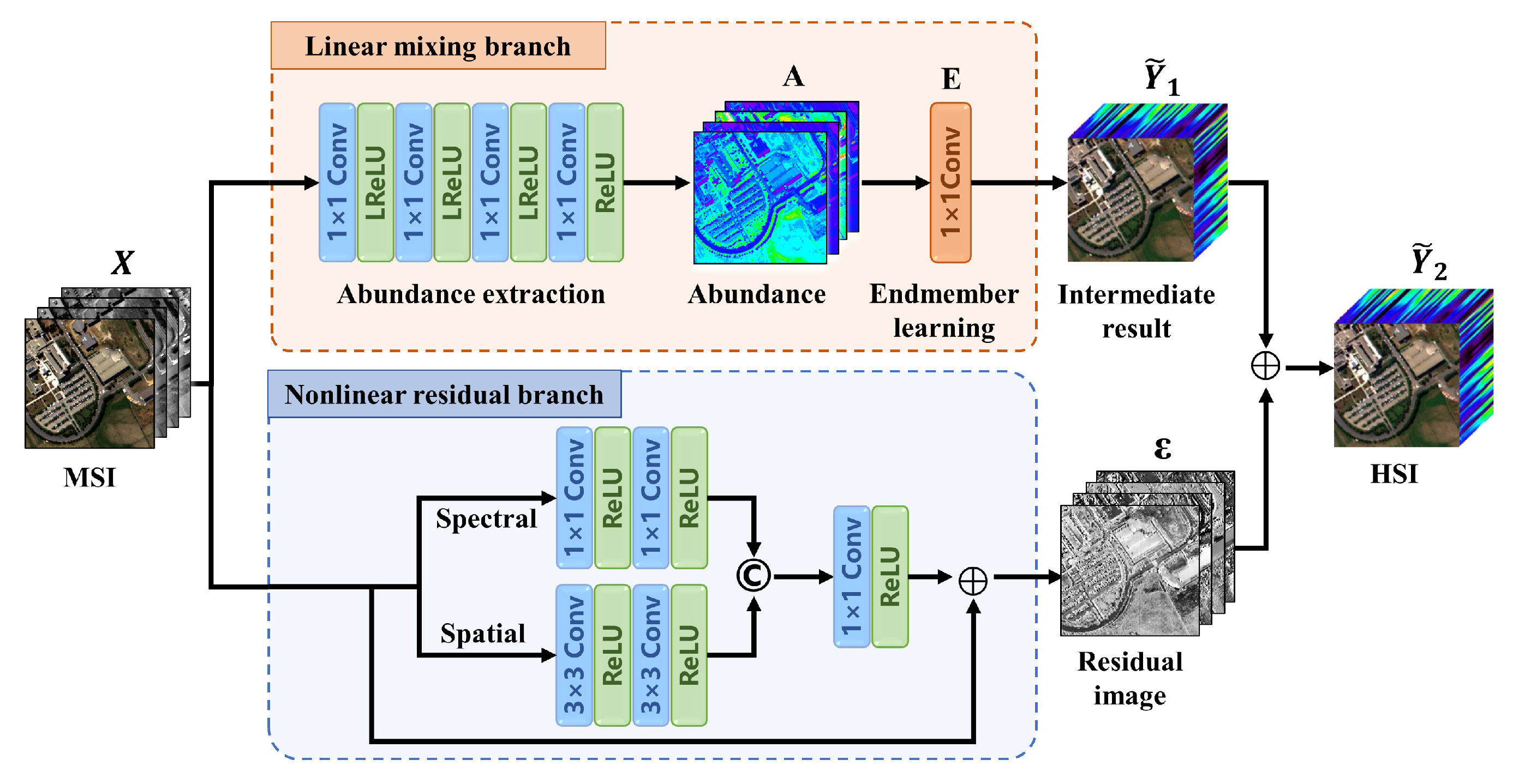
Based on the LSMM, a reasonable double-branch network is proposed to model the spectral mixing process in HSIs. Our network is trained on overlapping MSI–HSI image pairs and tested on non-overlapping MSIs. The framework is shown in Figure 2.
Inspired by the hyperspectral super-resolution method [37], the linear mixing branch consists of an abundance extraction module and an endmember adaptive learning layer. The input MSI is converted to a rough HSI as an intermediate result Y ˜ 1 R W × H × p of super-resolution through this branch.

2.2.1. Abundance Extraction Module

Based on the consistency of MSI–HSI abundances, this module aims to extract abundance from MSIs for the reconstruction of HSIs. Since linear unmixing is a pixel-wise decomposition operation, the kernel of the convolutional layers in this module is set to 1 × 1 . It can realize cross-channel information interaction and integration in the spectral dimension of the image. Meanwhile, training in a pixel-by-pixel way can reduce the interference of adjacent pixels on abundance extraction. Technically, the output channels can be set to the endmember number, which is controlled by the number of convolution kernels.
The activation function after the convolutional layer can greatly increase the feature extraction capability of the network and output an abundance map of MSIs. The first three convolution layers use the Leaky ReLU activation function. In contrast to a ReLU [38], a Leaky ReLU utilizes a near-zero coefficient to overcome the zero gradient problem of negative values [39]. Moreover, as mentioned before, the abundances need to satisfy two constraints, including the non-negative and sum-to-one constraints. In order to obtain the non-negative abundance image, the ReLU activation function is used in the last layer of this module to ensure that the output is greater than or equal to zero. As for the abundance sum-to-one constraint, we use the loss function to constrain the abundances and ensure the rationality of the abundance extraction. The specific calculation formula will be shown in the Joint Loss Function section.

2.2.2. Endmember Adaptive Learning

After the abundance extraction module, the hyperspectral endmembers are adaptively learned by a 1 × 1 2D convolutional layer. It is worth noting that endmembers are not feature maps extracted from MSIs but the weight parameters of the convolutional layer. The abundance map extracted from the previous module is mixed with the endmembers through the convolutional layer to output a rough HSI. The channel number of the convolution kernel is the same as the endmember number, and each kernel has p channels. The convolution kernel number is equal to HSI channel C, and each convolution kernel stores one hyperspectral endmember in an HSI. After training, the hyperspectral endmembers in the overlapping region are learned. In the test phase, the learned endmembers are directly loaded for the super-resolution of non-overlapping MSIs.
In the LSMM, the endmembers have a bounded non-negativity constraint in Equation (2). Therefore, the clamping function is exploited to limit the weights of the convolutional layer between 0 and 1. To further ensure that the linear branch learns effective endmembers and abundance, an HSI estimated loss function is added. The weight parameters are iteratively updated by back-propagation to minimize the error between rough HSIs and ground truth HSIs. By doing this, the linear branch provides a reliable foundation for the nonlinear branch.
The endmember number p should be determined before training, which is one of the important hyperparameters. As the weight of the network, endmembers are adaptive learners. The number of endmembers learned by the network p p . It is suggested that p should be set at a relatively big value to ensure all of the endmembers could be extracted.

2.3. Nonlinear Residual Branch

In addition to linear combination, there are residual ϵ formed by various nonlinear factors in the LSMM. Therefore, a single linear branch cannot perfectly represent the spectrum mixing process. In order to enhance the learning ability of nonlinear factors, a nonlinear residual branch is proposed to extract spatial and spectral features from MSIs. Spatial correlation is a very important attribute of remote sensing images, which is lacking in a linear branch. The information provided by the neighborhood of pixels is helpful in extracting fine spatial textures. For HSIs with continuous bands, the spectral correlation between adjacent bands is particularly obvious, which can be used to recover small waves on the spectral curve. We design a spatial module and a spectral module to extract spatial textures and spectral details, respectively.
In the first step, a 1 × 1 2D convolutional layer is used to upsample MSI spectral channels to 128, which is beneficial to extract rich features. Then, the spatial and spectral features are extracted in parallel. Specifically, two 3 × 3 convolutional layers and ReLUs constitute the spatial module to explore the complex nonlinear spatial structure. Two 1 × 1 convolutional layers and ReLUs constitute the spectral module to represent specific details in the spectral curve. In the SSR task, extracting the spectral feature after the spatial feature could result in feature confusion [29]. Therefore, we extract spectral and spatial features in parallel. By concatenating these two features, a spatial-spectral fusion feature with 256 channels can be obtained. Then, a 1 × 1 convolution and ReLU is added to further fuse spatial and spectral features, and the number of features is reduced to 128. After that, a skip connection is added to accelerate the convergence. Finally, nonlinear features are mapped into residual images with a 1 × 1 convolutional layer. The size and channels of residual images are the same as those of the HSIs.

2.4. Feature Fusion

According to the LSMM, the reconstruction of HSIs is dominated by linear mixing branches and supplemented by nonlinear branches. The linear branch plays a fundamental role by mixing endmembers and abundance to produce coarse intermediate results. The intermediate result is approximate to the real HSI but lacks some details. The nonlinear branch focuses on fine nonlinear features that are difficult to represent, such as high-frequency local spatial texture and spectral details. The nonlinear residual has both positive and negative values, and the value of most pixels should be close to zero, which plays the role of local adjustment and improvement. Adding the two kinds of images can further improve the accuracy of the intermediate results and obtain the final HSI Y ˜ 2 R W × H × p .

2.5. Joint Loss Function

In order to make these two branches play their respective roles, we constrain the network at different stages, including abundance extraction, intermediate result, and final result. The joint loss function consists of three parts.
  • Abundance sum-to-one error: As mentioned in the abundance extraction module, the abundance needs to meet the sum-to-one constraint, which means that the sum of an abundance of all endmembers in the pixel is 1. Therefore, we create a sum2one loss function to make the extracted abundance reasonable and efficient. To be specific, we sum the channel of the abundance image and calculate the difference between each pixel value and 1. The formula is as follows:
    L s u m 2 o n e = 1 i = 1 p A i 1
    where i indicates the ith band of the abundance matrix A.
  • HSI estimation error of intermediate result: The final result of this network is the fusion of linear and nonlinear branches. If we constrain the final result Y ˜ 2 but not the intermediate result Y ˜ 1 , each branch may fail to learn the desired result. Moreover, in traditional spectral unmixing, the error of image reconstruction is minimized to obtain the optimal endmembers and abundances. Therefore, it is necessary to constrain the intermediate result. In this way, when the model converges, the intermediate result Y ˜ 1 could be approximate to the real HSI Y and ensure the accuracy of endmember and abundance. The formula is as follows:
    L l i n e a r = Y Y ˜ 1 1
  • HSI estimation error of final result: The above two loss functions drive the gradient updating of the linear branch. In order to drive the nonlinear branch, the last HSI estimated loss function is added to the final result Y ˜ 2 . This loss promotes the learning of residual features and enhances the precision of super-resolution. The formula is as follows:
    L n o n l i n e a r = Y Y ˜ 2 1
Finally, the joint loss function L can be expressed as:
L = α L l i n e a r + β L n o n l i n e a r + γ L s u m 2 o n e
where α , β , and γ are the weight coefficients used to balance the errors.
Among the three loss functions, L s u m 2 o n e constrains the local abundance module of the network and accelerates abundance extraction. If the weight coefficient γ is too large, the network will pay more attention to the abundance and ignore the overall performance. Besides, the L l i n e a r and L n o n l i n e a r drive the two branches, respectively, which are the most important parts of the loss function. Correspondingly, parameters α and β should be larger than γ . As the important hyperparameters, the setting of these weights will be discussed later.

3. Results

3.1. Datasets

In addition to two classical simulated datasets, a real dataset is employed for experiments to comprehensively evaluate the performance of our network in practical applications.

3.1.1. Simulated Dataset

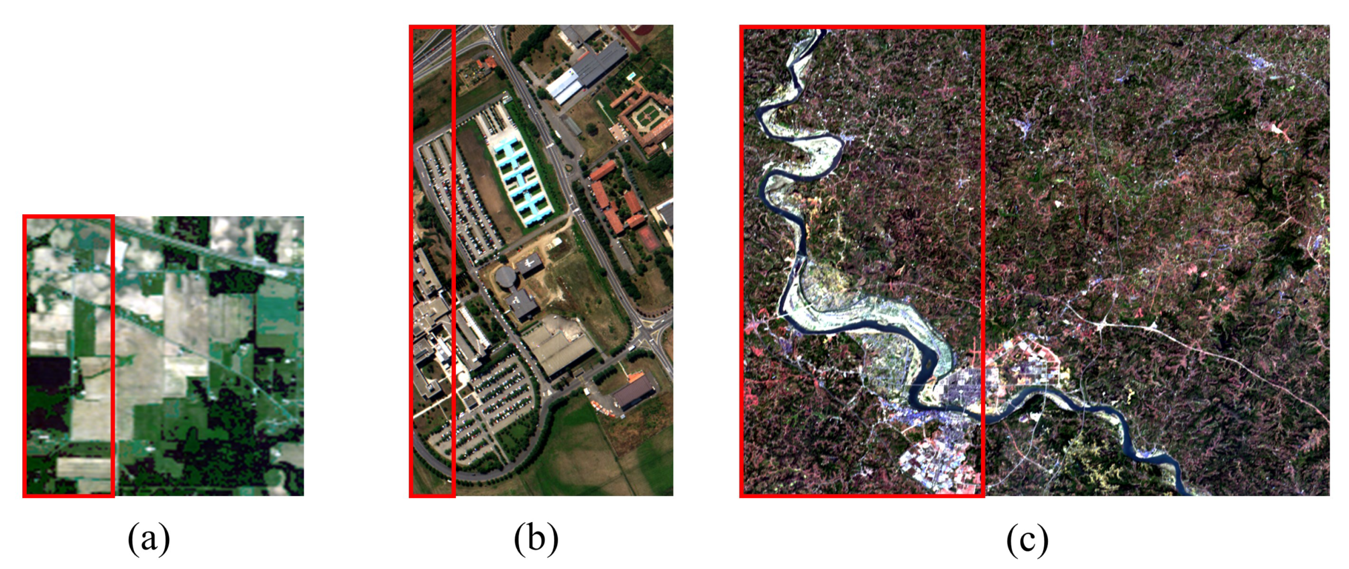
Considering the applicability of the spectral mixing model at different observation scales, two simulated data with different spatial resolutions are selected as shown in Figure 3. The Pavia University dataset, a commonly used high spatial resolution hyperspectral dataset, is employed to make a relatively fair comparison. In contrast, Indian pine data has a larger ground sample distance. There are no corresponding MSIs for these hyperspectral data, which need to be simulated through SRF and then used for SSR [40,41,42,43].
Pavia University dataset: This data was acquired by the Reflective Optics System Imaging Spectrometer (ROSIS) sensor in 2003 over Pavia, Italy, which is an airborne high-resolution HSI [44]. There are 610 × 340 pixels with a ground sampling distance of 1.3 m in the scene. The image has a spectral resolution of about 4 nm, covering the wavelength range from 430 to 860 nm, and the number of spectral channels is 115. Twelve of these bands are generally eliminated due to noise, so the remaining 103 bands are used for the experiment. The types of ground objects in the scene include artificial buildings, roads, vegetation, and soil. The spectral characteristics of various ground objects are quite different. Similar to many studies, we downsampled HSIs into 4 bands (i.e., the 450–520, 520–600, 630–690, and 760–900 nm domains) based on the SRF of QuickBird. In practice, the available MSI image covers a wide area, while the HSI only occupies a narrow part of the whole area. With reference to ZY1-02D satellite, the swath width of the MSI is twice that of the HSI. Therefore, we partition the test set larger than the training set to make it as realistic as possible and select 50 × 610 pixels on the left side of the image as the training set, and the rest as the test set. The specific situation of the study area is shown in Figure 3b.
Indian Pines dataset: This scene was gathered using an Airborne Visible/Infrared Imaging Spectrometer (AVIRIS) sensor over Indiana, USA. The image has 220 bands in the 400–2500 nm spectral range with a spatial resolution of about 20 m. It contains 145 × 145 pixels, two-thirds of which are agriculture and one-third of which is forest. Since the wavelength range of the hyperspectral data ranges from VIS to SWIR, Sentinel-2 is selected for spectral downsampling. We simulated MSIs with 13 bands, which provides more spectral information than QuickBird. The division of the training set and test set follows the same principle. The 45 × 145 pixels on the left are the training set, and the rest are the test set, as shown in Figure 3a.

3.1.2. Real Satellite Dataset

In fact, the simulated datasets can not reflect the real state of ground objects and image quality in practical application. The spatial positions of each MSI–HSI pixel pair in the simulated dataset correspond exactly, but there is an inevitable registration error between the MSI and the HSI in the actual observation. In addition, due to the sensor system, the hyperspectral satellite data may have periodic noise. In order to reduce the impact of registration, a pair of MSI–HSI images observed simultaneously by the Chinese ZY1-02D satellite were selected to carry out the experiment in a larger area.
The ZY1-02D satellite was launched by China in 2019, carrying a visible near-infrared camera (VNIC) and an advanced hyperspectral imager (AHSI). It can simultaneously observe MSIs with 8 bands from visible to near-infrared (i.e., the 452–521, 522–607, 635–694, 776–895, 416–452, 591–633, 708–752, and 871–1047 nm domains) and 166 bands of HSIs from visible to shortwave infrared (395–2500 nm) [45]. According to the wavelength range of MSIs, we only extend the spectrum of MSIs to the corresponding 94 bands (395–1341 nm) of HSIs. The original data were preprocessed with radiometric calibration, atmospheric correction, and image registration to obtain the reflectance image. The MSI spatial resolution is 10 m, and the HSI spatial resolution is 30 m. To keep the same ground sampling distance between MSIs and HSIs, pixel aggregation is used to down-sample MSI to 30 m resolution. A large area with 800 × 1000 pixels was selected, which included a lot of vegetation and a few cities and water bodies. The training set was 800 × 150 pixels in the study area, which contained as many ground object types as possible. As shown in Figure 3c.

3.2. Implementation Details

Considering the characteristics of hyperspectral images, the performance of spectral super-resolution methods is evaluated using five indexes, including root mean square error (RMSE), peak signal-to-noise ratio (PSNR), spectral angle mapper (SAM), structural similarity index(SSIM), and erreur relative globale adimensionnelle de synthèse (ERGAS), from different perspectives [46,47]. The RMSE and PSNR calculate the error of pixel value without considering the neighborhood information. SSIM pays more attention to the similarity of the local spatial structure of images. SAM evaluates the similarity of spectral curve shape and trend, reflecting the quality of spectral feature recovery. Based on the RMSE of each band, ERGAS considers the mean reflectance and synthesizes the overall variation of the spectrum for evaluation.
The proposed model is trained with an Adam optimizer. The training epoch was set to 5000, and the initial learning rate was set to 0.003. After 1000 epochs, the learning rate starts to decay linearly until it is reduced to zero in the last epoch. Our experiments do not crop the data into patches. We directly input the complete image to the network, so the batch size was 1. We set the number of endmembers p for each dataset, where p = 20 for Pavia dataset and p = 30 for the Indian pine and ZY1-02D datasets. The trade-off parameter ratio of the loss function was set to 100:1:100. Our model was trained using the PyTorch deep learning framework.

3.3. Comparison with the State of the Art

In this section, we compare the proposed method with four state-of-the-art methods mentioned before, including CanNet [26], HSCNN+ [27], J-SLoL [20], and SSRAN [33]. Among them, J-SLoL is a sparse representation method, while the others are deep learning methods. CanNet and HSCNN+ are representative methods in the NTIRE 2018 Spectral Reconstruction Challenge [47]. CanNet is a shallow CNN residual network. HSCNN+ is the competition winner with a densely-connected structure. SSRAN is proposed in 2022 to simultaneously extract features from spatial and spectral dimensions. Among them, HSCNN+, and SSRAN have classical structures in SSR networks, including the feature extraction part, the nonlinear mapping part, and the reconstruction part.
The hyperparameters of J-SLoL are set according to the original literature. In the Spectral Reconstruction Challenge, HSCNN+ used 160 densely connected blocks. To make a fair comparison, we reduce the number of densely connected blocks to 20 so that the number of HSCNN+ parameters is roughly equivalent to that of the proposed network. The learning rates of HSCNN+, CanNet, and SSRAN are the same as the settings of the original literature. Their training epoch and batch size are the same as the settings of the proposed method. The visual and quantitative performance of the spectral superresolution results is shown as follows.

3.3.1. Results Using Pavia University Dataset

The quantitative results of the five methods on the Pavia university dataset are shown in Table 2. It is found that the deep learning method has better performance than the sparse representation method in terms of SAM, SSIM, and ERGAS. The sparse representation method is trained pixel by pixel, which disrupts the spatial structure of the image and cannot reflect the spatial correlation. In deep learning networks, CanNet and HSCNN+ have achieved acceptable results. Due to its deep structure, HSCNN+ shows higher accuracy than CanNet in all aspects, which is second only to the proposed method. Among all the methods, the proposed network achieves excellent performance in both spatial and spectral evaluation. Compared with the suboptimal method, our method has a significant improvement of about 0.14 SAM, 1.35 PSNR, 0.002 SSIM, 0.3 RMSE, and 1 EGRGAS. The results demonstrate the high spatial and spectral fidelity of the proposed method in SSR.
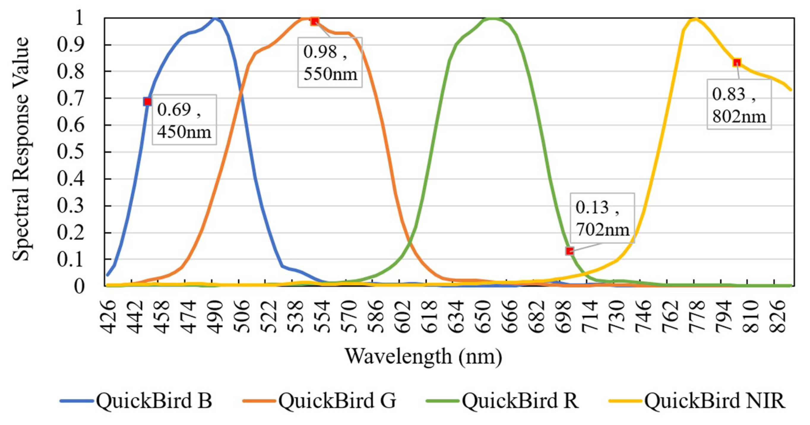
Figure 4 shows the single band error and the RMSE and SAM errors of the image cube. Columns 1 to 4 are the errors of HSI reconstruction at 450 nm, 550 nm, 702 nm, and 802 nm, respectively. Compared with other wavelengths, the reconstruction error at 702 nm is the largest due to the limited spectral information of MSIs. According to the SRF of the QuickBird sensor Figure 5, 702 nm is at the edge of the MSI spectral coverage. Therefore, MSIs can not reflect the spectral characteristics of HSIs at 702 nm, which makes it difficult to reconstruct the image. From the comparison of methods, J-SLoL is a model-driven model among the state-of-the-art methods, which can better retain the original spectral information provided by MSIs. By contrast, data-driven deep learning has a better fitting ability for bands lacking reference information. The results show that J-SLoL performs well at 550 nm and 802 nm near the central wavelength of the MSI, but its error at 702 nm is larger than that of the deep learning method. Additionally, the RMSE of the buildings shown in the red rectangle is poor due to the fact that the corresponding objects are not covered in the training images. Nevertheless, our approach performs well in local building areas and has the smallest RMSE and SAM in the entire study area.

3.3.2. Results Using Indian Pines Dataset

Using the Indian Pines dataset, the quantitative evaluations of the five approaches are displayed in Table 3. The input MSI with 13 bands greatly reduces the difficulty of HSI recovery, so the overall accuracy of Indian Pines data is higher than that of Pavia data. The strengths and weaknesses of the comparison algorithm on the two datasets are basically the same. The performance of the deep learning method in SAM, SSIM, and ERGAS is better than that of the sparse representation method. In particular, HSCNN+ is superior in SAM with an increase of 0.14 compared with the proposed method. However, other indexes of this method are lower than that of the proposed model, such as the PSNR decreasing by 3.95. In other respects, our method still achieves outstanding results.
Figure 6 shows the single band and overall effect of the comparison methods using the Indian Pines dataset. Firstly, we analyze the reconstruction effects at different wavelengths. The ground objects in this data are mainly vegetation, whose reflectance is greatly reduced due to the absorption of water vapor in the short-wave infrared (SWIR). Moreover, the spectral curve of vegetation is relatively flat in SWIR. The reflectance of Sentinel-2 MSIs at 1376.9 nm, 1610.4 nm, and 2185.7 nm can record typical spectral characteristics, which are sufficient to recover HSIs in SWIR. Accordingly, the five methods show excellent performance in SWIR, as shown in columns 4 to 6 of the Figure 6. In addition, the reconstruction accuracy of different ground objects is different. In the 1000 nm, the ground objects in the red box are roads and hay. The training image does not contain these two types of ground objects, resulting in a poor reconstruction effect. Additionally, the proposed method has a darker blue color in the red box in the RMSE and SAM heat maps, indicating superior performance.

3.3.3. Results on ZY1-02D Dataset

Table 4 reports the results on the ZY1-02D dataset. Compared with the simulated dataset in the ideal state, the real dataset inevitably has MSI and HSI registration errors. The stability and robustness of the model can be tested by this data. For the real satellite dataset, our method specifically adds a 5 × 5 convolution layer to expand the receptive field at the beginning of the linear mixing branch. The results show that the performance of sparse representation methods on real datasets is seriously affected. The mismatch of one or two pixels will greatly reduce the accuracy of J-SLoL. On the contrary, the deep learning-based method has a larger receptive field, which is more suitable for the real dataset with registration errors. In this paper, the proposed method combines the advantages of deep learning, further makes up for the limitations of the physical model, and shows strong robustness on both real and simulated data sets.
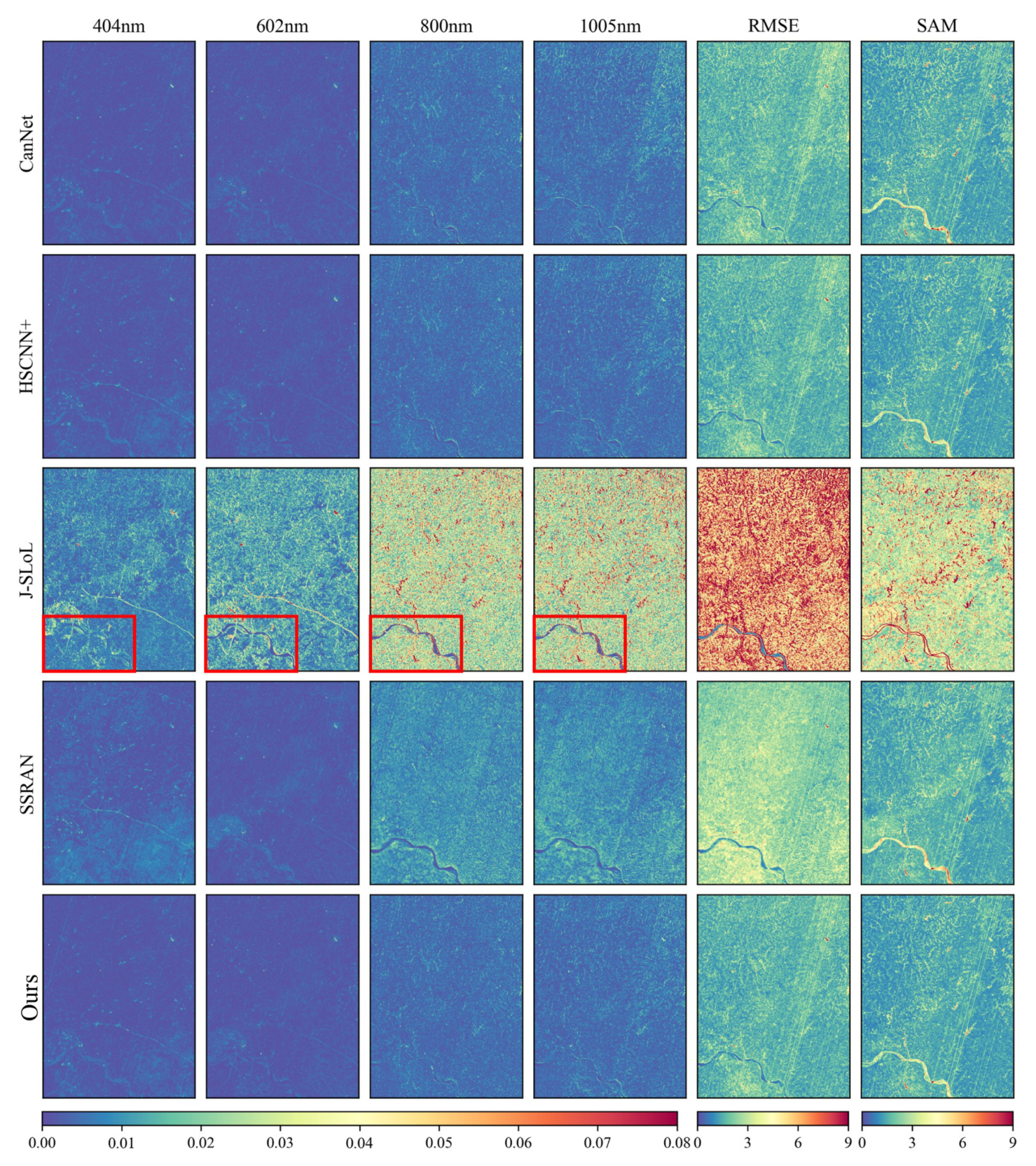
Figure 7 shows the single band and overall performance on the ZY1-02D dataset. The MSI–HSI pixel pairs in the simulated dataset correspond exactly to each other, which cannot reflect the registration problem. Therefore, we visually analyze experimental results on the real data to evaluate the performance of the model in a practical application. In fact, the traditional method has a high requirement for spatial position matching of MSI–HSI image pairs. As a result, the performance of J-SLoL with real data sets is unstable, especially in the junction between the river banks and vegetation in the red box in Figure 7. Due to the low spatial resolution of satellite data, there are many mixed pixels at the boundary of the river. The spectral mismatch of MSI–HSI pixel pairs results in a poor representation of mixed pixels in the model. At 404 nm and 602 nm, the spectral curves of the river and nearby vegetation are similar, with reflectance below 0.1. In these bands, the spectra of the two objects are basically unchanged after mixing, so the registration error has little influence on the image reconstruction. At 800 nm and 1005 nm, vegetation has high reflectance, while river reflectance is close to 0. In these two bands, the spectral difference between the mixed pixels and the pure objects is very obvious. Therefore, it is difficult to reconstruct the spectrum when MSI–HSI pixel pairs do not match. In this case, the accuracy of the proposed method remains stable and is the best of all methods. In addition, the interference of striping noise can be clearly observed in the RMSE and SAM maps. It can be seen that periodic noise in real data is more serious than that in simulated data. In general, our method has strong robustness and universality to real data in practical applications.

3.4. Visualization Results

This section takes the Pavia University dataset as an example to show the internals of the proposed network, such as the endmembers and the abundances extracted by the network, and the output of the two branches.

3.4.1. Endmembers and Abundances

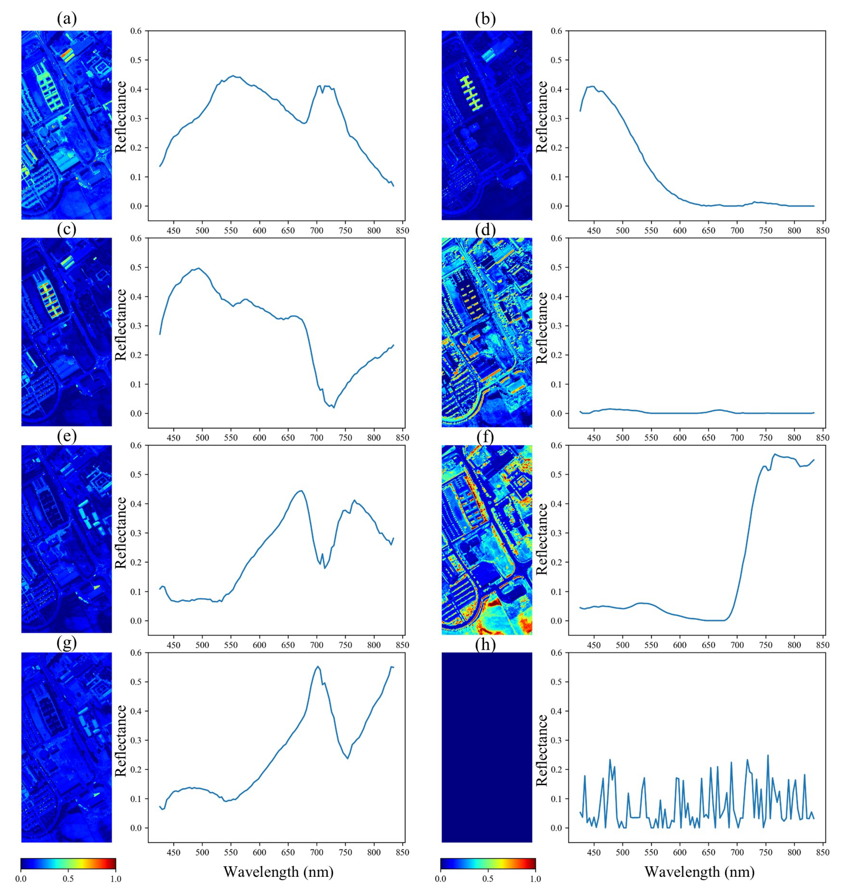
The original intention of the linear mixing branch was to extract endmembers and abundance. Therefore, we show the hyperspectral endmembers and the abundance of the Pavia University dataset extracted by the network in Figure 8. Spectral unmixing is an ill-posed problem whose solution is not unique. Since deep learning has a certain randomness, the endmembers, and abundance extracted from the network are likely to be different from the solution of the physical model. The network extracts seven valid endmembers and the corresponding abundance maps from the Pavia University dataset. In most cases, people assume that a ground object has only one endmember spectral in a remote sensing image. However, according to the abundance distribution, the three spectral curves in Figure 8a–c are simultaneously used to recover the blue and white roofs in the true color image. This phenomenon can be explained by spectral variability, in which the reflectivity of the same material changes with the environment. Similarly, the endmembers in Figure 8e,g reconstruct the red roof in the true color image together. The abundance Figure 8d represents the shadows of buildings and trees and other ground objects with low reflectance. Finally, the abundance in Figure 8f extracts the vegetation distribution, and the corresponding endmembers contain spectral characteristics of the vegetation visibly.
Since the number of endmembers is unknown, we set the parameter p = 20 before training. After adaptive learning, the number of effective endmembers p 20 , and the rest endmembers were invalid. As shown in Figure 8h, the invalid end member did not learn obvious spectral features, so it presented an irregular curve. The corresponding abundance value of these invalid endmembers was zero. Therefore, an invalid endmember multiplied by abundance will not affect the final result.

3.4.2. Results of Two Branches

Since the final result is the fusion of two branches, we show the output of each branch in Figure 9a,b to explore their roles. We find that the intermediate result of the linear branch is close to the ground truth HSI. This branch reconstructs the structure of HSI, which is the major part of the whole network. Meanwhile, the amplitude of the residual image is marginal ( ± 0.25 ), which indicates that the nonlinear branch works as a fine-tuning to the linear branch. Specifically, we select a roof region to exhibit the minor difference between the intermediate and final results. The reconstruction of the selected region is difficult since the spectrum of uneven roofs varies widely within tiny spatial fluctuations. Therefore, we draw the spectral curves of a roof pixel in Figure 9c,d. The spectral trend in the intermediate result is similar to that of the real HSI. But there still exists small reflectance difference between them. After the adjustment of the nonlinear residual branch, the spectral curve becomes visibly closer to the real HSI, which further improves the performance.

3.5. Ablation Study

To validate the effectiveness of the double-branch structure, we test the performance of the networks with a single linear mixing branch and a single nonlinear residual branch. In the single linear mixing branch, the loss function includes the HSI estimation error, and the abundance sum-to-one constraint. The coefficients α and γ are 100 and 1, respectively. In the single nonlinear branch, only the HSI estimation error is calculated. The rest of the hyperparameters are kept per Section 3.2.
Table 5 reports the results of single-branch and double-branch on three datasets. Compared with the double-branch network, the accuracy of the single linear branch is lower on three datasets, with a comprehensive decrease of 0.31 SAM, 1.55 PSNR, 0.01 SSIM, 0.54 RMSE, and 0.89 ERGAS. The single nonlinear branch without a linear branch performs worse than the double-branch network with 0.03 SAM, 0.31 PSNR, 0.0006 SSIM, 0.09 RMSE, and 0.23 ERGAS. On two simulated datasets, the performance of the single linear branch is competitive with other advanced methods. In this case, the nonlinear branch further improves the accuracy of the model and achieves superior results. However, due to the more severe nonlinearity of the real dataset, the performance of the single linear branch is affected. Supplemented by the nonlinear branch, the double-branch results are significantly enhanced on the ZY1-02D dataset. It can be seen that the two branches can complement and promote each other in the double-branch structure. Specifically, the linear branch provides an acceptable foundation for the nonlinear branch. Then, the nonlinear branch focuses on the learning of residuals and effectively supplements the spatial and spectral characteristics of the linear branch.

3.6. Time Cost

In this article, all methods are validated on a workstation with an Intel Xeon Platinum 8358 CPU, 512 GB RAM, NVIDIA RTX A6000, and a Windows system. CanNet, HSCNN+, SSRAN, and our method are executed in the PyTorch framework and GPU. Specifically, the J-SLoL is the sparse representation method, which is evaluated using public MATLAB projects. To investigate the efficiency of SSR application on a large scale, we reported the training time of different methods on the ZY1-02D dataset. As shown in Table 6, we found that the training time of sparse representation was longer than that of deep learning. As the dataset got larger, the J-SLoL required more time to extract the appropriate MSI and HSI dictionaries. In deep learning methods, most of them spent less than half an hour on training. Relatively speaking, our method can achieve the highest accuracy with acceptable time consumption.

4. Discussion

This section conducts experiments on the most important hyperparameters in this network. We discuss the influence of the number of endmembers and the weights of loss functions on SSR.

4.1. Number of Endmembers

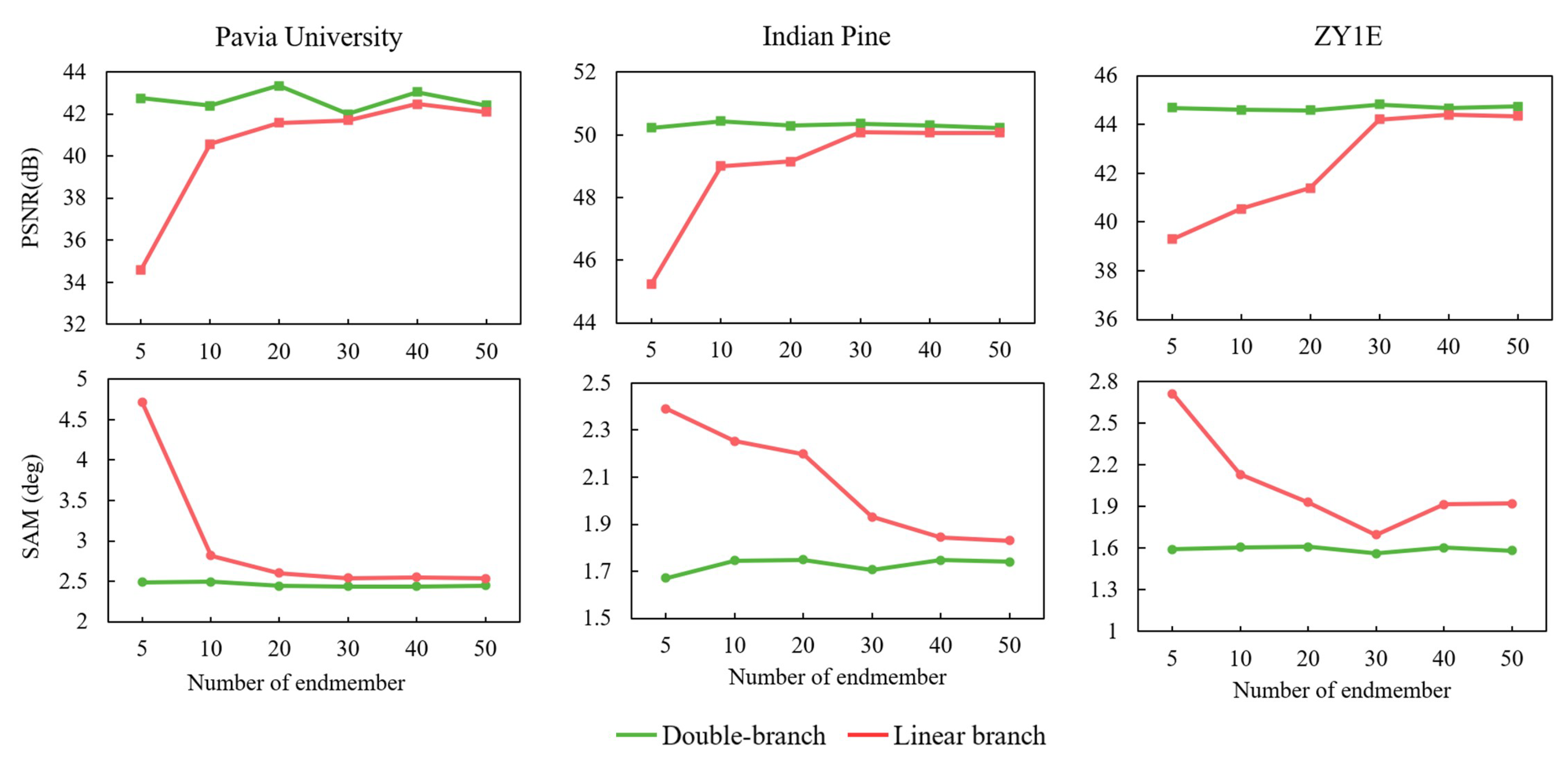
The endmembers are set as 5, 10, 20, 30, 40, and 50. Figure 10 shows the variations of PSNR and SAM with different endmember numbers on three datasets. The orange curve represents the PSNR or SAM of the linear branch, and the blue curve indicates the PSNR or SAM of the double-branch network. It can be found that the linear mixing branch is sensitive to the endmember number. The linear branch performs worse when the endmember number is set to 5 because the endmembers are too few to contain all types of objects in the image. In comparison, the double-branch structure shows strong robustness to the endmember number. When the endmembers increase from 5 to 50, the double-branch network performs stable and keeps high performance due to the supplement of the nonlinear branch.
In addition, the index of the linear branch indicates that the performance of this branch improves with the increase of the endmember number until convergence. Different datasets have different convergence conditions. For the Pavia University dataset, a satisfactory result can be obtained on the linear branch when the endmember is set to 20. Furthermore, the PSNR increases rapidly, and the SAM decreases rapidly because there are not many types of ground objects in this dataset. In contrast, the Indian Pine dataset converges slowly, and the performance becomes stable until the endmember is 30. However, the indexes of this dataset are superior to those of the Pavia University dataset from the start. The main reason is that the ground objects have similar spectra and the corresponding MSI contains more bands in this dataset that are beneficial to HSI reconstruction. On this basis, in order to provide a better foundation for the nonlinear branch, the linear branch requires more endmembers to converge completely. Due to the large size of real data, the convergence of PSNR and SAM is more difficult than that of simulated data in the linear branch. For example, the SAM of this branch increases when the endmember number is greater than 30. However, from the perspective of double-branch results, the stability of real data is better than that of the simulated data. We compared the blue curves of the three datasets. Specifically, the amplitudes of PSNR in the Pavia University dataset and SAM in the Indian Pine dataset are both larger than those of the ZY1-02D data. This rich data provides comprehensive training samples for the nonlinear branch so that the PSNR and SAM of the double-branch network remain stable under different endmember numbers.

4.2. Loss Function Weight Coefficients

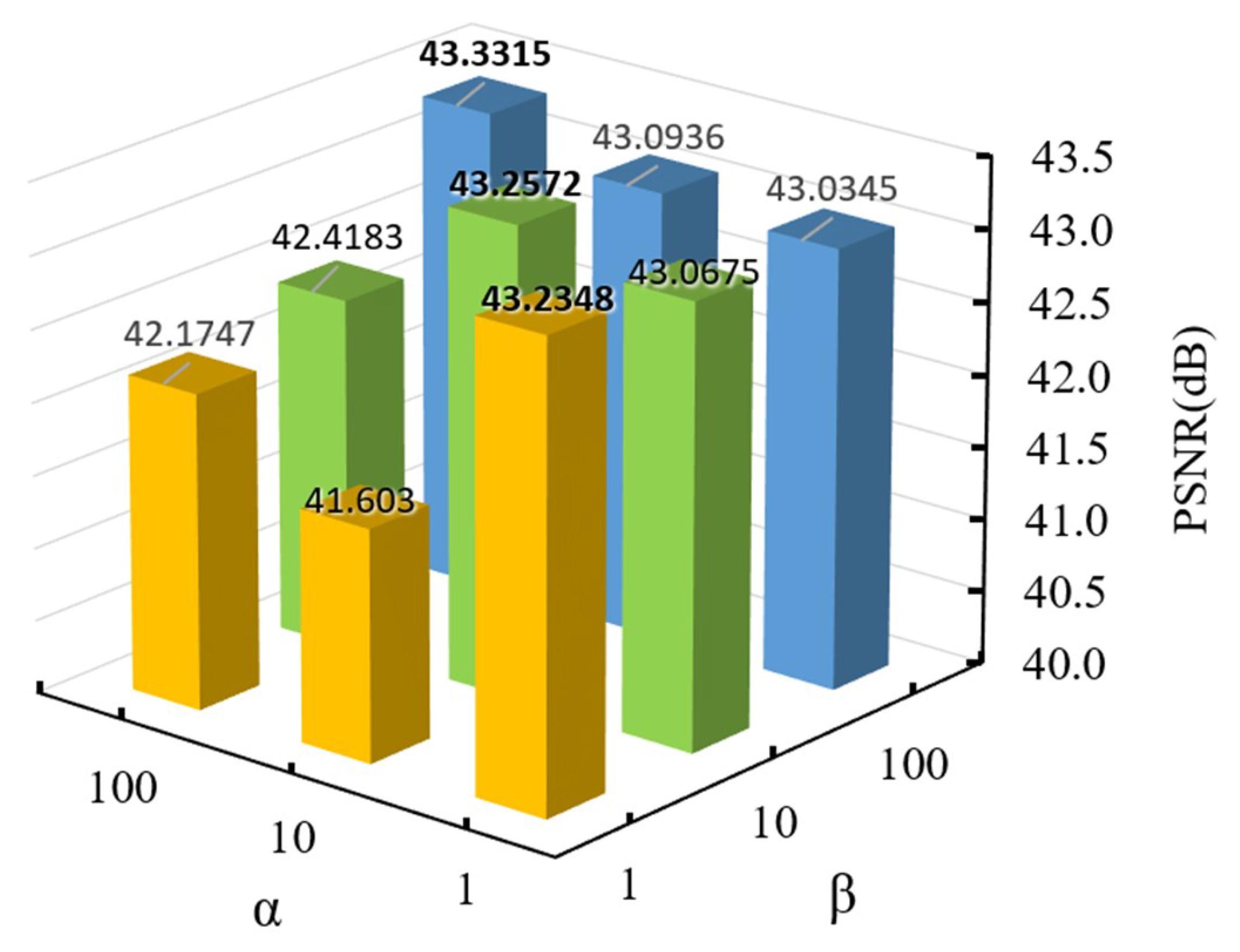
In the joint loss function, the weight coefficients contain α , β , and γ . α and β are used to balance the HSI reconstruction error of the two branches, and γ is the weight of the abundance sum-to-one constraint. α and β are the main factors affecting the reconstruction results, while γ plays an auxiliary role, which is set to 1. On this basis, we further test the appropriate proportional coefficients α and β .
Figure 11 shows the PSNR of the Pavia University data when α and β are 1, 10, and 100. We found that both parameters have effects on the experimental results. In fact, simply increasing these two parameters does not always lead to better results. For example, when β is set to 100, PSNR improves as α increases. However, when β is set to 1, we find that increasing α will lead to worse results. The best result is when α is set to 1. In summary, it can be concluded that the performance of our network will be better when α and β are equal. In other words, the linear and nonlinear branches work best when they have the same weight. In addtion, it can be seen that the PSNR is lower when α is greater than β . The reason is that the linear branch has limited learning ability. When α is greater than β , the network pays more attention to recovering rough spectral trends and spatial structure of the image with the linear branch. In this case, the nonlinear branch is ignored, resulting in a lack of fine spatial and spectral characteristics. When β is larger than α , the nonlinear branch plays a dominant role. Although the linear branch does not achieve the best performance in this case, the nonlinear branch with strong learning ability can complement the remaining features. In this way, the final accuracy of HSIs will always be maintained at a high level. Finally, this experiment shows that the best performance is achieved when α = β = 100 . Therefore, the coefficients α = β = 100 and γ = 1 are determined in all our experiments.

5. Conclusions

In this paper, we propose a reasonable double-branch SSR network to transform MSIs into HSIs. We introduced the linear spectral mixing theory and prior knowledge in remote sensing to instruct the design of the model structure. Using a linear mixing branch, we can obtain acceptable rough HSIs. The nonlinear branch further complements the detailed information for the rough HSIs. In addition, hyperspectral endmembers and abundance can be extracted through the network. Experiments on simulated and real datasets show that the double-branch network significantly improves the reconstruction accuracy and robustness. The previous work assumes that the ground object types in the training dataset are consistent with those in the test dataset. This hypothesis limits the performance of SSR models, especially in large areas. In future work, we will pay more attention to this problem. In addition, we intend to analyze the performance of SSR methods on different classes of ground objects in detail in the following work.

Author Contributions

Conceptualization, L.S. and W.Z.; Data curation, Z.L. (Zhen Li); Investigation, B.Z.; Methodology, L.S. and W.Z.; Resources, B.Z.; Software, L.S. and Z.L. (Zhiqiang Liu); Visualization, L.S.; Writing—original draft, L.S.; Writing—review and editing, W.Z. and Z.L. (Zhiqiang Liu). All authors have read and agreed to the published version of the manuscript.

Funding

This research was funded by the Youth Innovation Promotion Association, CAS, the National Natural Science Foundation of China (NSFC no. 41042201503), and the Defense Industrial Technology Development Program.

Data Availability Statement

Acknowledgments

The authors would like to thank Ke Zheng at the College of Geography and Environment, Liaocheng University, China, for valuable discussions on topics related to this work.

Conflicts of Interest

The authors declare no conflict of interest.

References

  1. Zhang, L.; Li, J. Development and Prospect of Sparse Representation-Based Hyperspectral Image Processing and Analysis. J. Remote Sens. 2016, 20, 1091. [Google Scholar] [CrossRef]
  2. Goetz, A.F.H.; Vane, G.; Solomon, J.E.; Rock, B.N. Imaging Spectrometry for Earth Remote Sensing. Science 1985, 228, 1147–1153. [Google Scholar] [CrossRef] [PubMed]
  3. Siebels, K.; Goïta, K.; Germain, M. Estimation of Mineral Abundance From Hyperspectral Data Using a New Supervised Neighbor-Band Ratio Unmixing Approach. IEEE Trans. Geosci. Remote Sens. 2020, 58, 6754–6766. [Google Scholar] [CrossRef]
  4. Thiemann, S.; Kaufmann, H. Lake water quality monitoring using hyperspectral airborne data—A semiempirical multisensor and multitemporal approach for the Mecklenburg Lake District, Germany. Remote Sens. Environ. 2002, 81, 228–237. [Google Scholar] [CrossRef]
  5. Yuan, Q.; Shen, H.; Li, T.; Li, Z.; Li, S.; Jiang, Y.; Xu, H.; Tan, W.; Yang, Q.; Wang, J.; et al. Deep learning in environmental remote sensing: Achievements and challenges. Remote Sens. Environ. 2020, 241, 111716. [Google Scholar] [CrossRef]
  6. Zhang, N.; Yang, G.; Pan, Y.; Yang, X.; Chen, L.; Zhao, C. A Review of Advanced Technologies and Development for Hyperspectral-Based Plant Disease Detection in the Past Three Decades. Remote Sens. 2020, 12, 3188. [Google Scholar] [CrossRef]
  7. Yu, H.; Zhang, H.; Liu, Y.; Zheng, K.; Xu, Z.; Xiao, C. Dual-Channel Convolution Network with Image-Based Global Learning Framework for Hyperspectral Image Classification. IEEE Geosci. Remote Sens. Lett. 2022, 19, 1–5. [Google Scholar] [CrossRef]
  8. Yokoya, N.; Yairi, T.; Iwasaki, A. Coupled non-negative matrix factorization (CNMF) for hyperspectral and multispectral data fusion: Application to pasture classification. In Proceedings of the 2011 IEEE International Geoscience and Remote Sensing Symposium, Vancouver, BC, Canada, 24–29 July 2011; pp. 1779–1782. [Google Scholar] [CrossRef]
  9. Manolakis, D.; Shaw, G. Detection algorithms for hyperspectral imaging applications. IEEE Signal Process. Mag. 2002, 19, 29–43. [Google Scholar] [CrossRef]
  10. Nielsen, A.A. The Regularized Iteratively Reweighted MAD Method for Change Detection in Multi- and Hyperspectral Data. IEEE Trans. Image Process. 2007, 16, 463–478. [Google Scholar] [CrossRef] [Green Version]
  11. Xu, Y.; Wu, Z.; Chanussot, J.; Comon, P.; Wei, Z. Nonlocal Coupled Tensor CP Decomposition for Hyperspectral and Multispectral Image Fusion. IEEE Trans. Geosci. Remote Sens. 2020, 58, 348–362. [Google Scholar] [CrossRef]
  12. Yang, J.; Zhao, Y.Q.; Chan, J.C.W. Hyperspectral and Multispectral Image Fusion via Deep Two-Branches Convolutional Neural Network. Remote Sens. 2018, 10, 800. [Google Scholar] [CrossRef] [Green Version]
  13. Li, J.; Bioucas-Dias, J.M.; Plaza, A. Spectral–Spatial Hyperspectral Image Segmentation Using Subspace Multinomial Logistic Regression and Markov Random Fields. IEEE Trans. Geosci. Remote Sens. 2012, 50, 809–823. [Google Scholar] [CrossRef]
  14. Zhong, Y.; Wang, X.; Wang, S.; Zhang, L. Advances in spaceborne hyperspectral remote sensing in China. Geo-Spat. Inf. Sci. 2021, 24, 95–120. [Google Scholar] [CrossRef]
  15. Mei, S.; Jiang, R.; Li, X.; Du, Q. Spatial and Spectral Joint Super-Resolution Using Convolutional Neural Network. IEEE Trans. Geosci. Remote Sens. 2020, 58, 4590–4603. [Google Scholar] [CrossRef]
  16. Chen, W.; Zheng, X.; Lu, X. Semisupervised Spectral Degradation Constrained Network for Spectral Super-Resolution. IEEE Geosci. Remote Sens. Lett. 2022, 19, 1–5. [Google Scholar] [CrossRef]
  17. He, J.; Li, J.; Yuan, Q.; Shen, H.; Zhang, L. Spectral Response Function-Guided Deep Optimization-Driven Network for Spectral Super-Resolution. IEEE Trans. Neural Networks Learn. Syst. 2022, 33, 4213–4227. [Google Scholar] [CrossRef] [PubMed]
  18. Arad, B.; Ben-Shahar, O. Sparse Recovery of Hyperspectral Signal from Natural RGB Images. In Proceedings of the Computer Vision, ECCV 2016, Amsterdam, The Netherlands, 11–14 October 2016; Leibe, B., Matas, J., Sebe, N., Welling, M., Eds.; Springer International Publishing: Cham, Switzerland, 2016; pp. 19–34. [Google Scholar]
  19. Rubinstein, R.; Zibulevsky, M.; Elad, M. Efficient Implementation of the K-SVD Algorithm Using Batch Orthogonal Matching Pursuit; Technical report; Computer Science Department, Technion: Haifa, Israel, 2008. [Google Scholar]
  20. Gao, L.; Hong, D.; Yao, J.; Zhang, B.; Gamba, P.; Chanussot, J. Spectral Superresolution of Multispectral Imagery with Joint Sparse and Low-Rank Learning. IEEE Trans. Geosci. Remote Sens. 2021, 59, 2269–2280. [Google Scholar] [CrossRef]
  21. Huang, Z.; Chen, Q.; Chen, Q.; Liu, X.; He, H. A Novel Hyperspectral Image Simulation Method Based on Nonnegative Matrix Factorization. Remote Sens. 2019, 11, 2416. [Google Scholar] [CrossRef] [Green Version]
  22. Nguyen, R.M.H.; Prasad, D.K.; Brown, M.S. Training-Based Spectral Reconstruction from a Single RGB Image. In Proceedings of the Computer Vision, ECCV 2014, Zurich, Switzerland, 6–12 September 2014; Fleet, D., Pajdla, T., Schiele, B., Tuytelaars, T., Eds.; Springer International Publishing: Cham, Switzerland, 2014; pp. 186–201. [Google Scholar]
  23. Alvarez-Gila, A.; van de Weijer, J.; Garrote, E. Adversarial Networks for Spatial Context-Aware Spectral Image Reconstruction from RGB. CoRR 2017, arXiv:1709.00265. [Google Scholar]
  24. Jégou, S.; Drozdzal, M.; Vazquez, D.; Romero, A.; Bengio, Y. The One Hundred Layers Tiramisu: Fully Convolutional DenseNets for Semantic Segmentation. In Proceedings of the 2017 IEEE Conference on Computer Vision and Pattern Recognition Workshops (CVPRW), Honolulu, HI, USA, 21–26 July 2017; pp. 1175–1183. [Google Scholar] [CrossRef] [Green Version]
  25. Galliani, S.; Lanaras, C.; Marmanis, D.; Baltsavias, E.; Schindler, K. Learned Spectral Super-Resolution. CoRR 2017, arXiv:1703.09470. [Google Scholar]
  26. Can, Y.B.; Timofte, R. An efficient CNN for spectral reconstruction from RGB images. CoRR 2018, arXiv:1804.04647. [Google Scholar]
  27. Shi, Z.; Chen, C.; Xiong, Z.; Liu, D.; Wu, F. HSCNN+: Advanced CNN-Based Hyperspectral Recovery from RGB Images. In Proceedings of the 2018 IEEE/CVF Conference on Computer Vision and Pattern Recognition Workshops (CVPRW), Salt Lake City, UT, USA, 18–22 June 2018; pp. 1052–10528. [Google Scholar] [CrossRef]
  28. Li, J.; Wu, C.; Song, R.; Li, Y.; Xie, W.; He, L.; Gao, X. Deep Hybrid 2-D-3-D CNN Based on Dual Second-Order Attention with Camera Spectral Sensitivity Prior for Spectral Super-Resolution. IEEE Trans. Neural Netw. Learn. Syst. 2021, 34, 623–634. [Google Scholar] [CrossRef] [PubMed]
  29. Li, J.; Wu, C.; Song, R.; Xie, W.; Ge, C.; Li, B.; Li, Y. Hybrid 2-D–3-D Deep Residual Attentional Network with Structure Tensor Constraints for Spectral Super-Resolution of RGB Images. IEEE Trans. Geosci. Remote Sens. 2021, 59, 2321–2335. [Google Scholar] [CrossRef]
  30. Ji, S.; Xu, W.; Yang, M.; Yu, K. 3D Convolutional Neural Networks for Human Action Recognition. IEEE Trans. Pattern Anal. Mach. Intell. 2013, 35, 221–231. [Google Scholar] [CrossRef] [PubMed] [Green Version]
  31. Mei, S.; Ji, J.; Hou, J.; Li, X.; Du, Q. Learning Sensor-Specific Spatial-Spectral Features of Hyperspectral Images via Convolutional Neural Networks. IEEE Trans. Geosci. Remote Sens. 2017, 55, 4520–4533. [Google Scholar] [CrossRef]
  32. Arun, P.V.; Herrmann, I.; Budhiraju, K.M.; Karnieli, A. Convolutional network architectures for super-resolution/sub-pixel mapping of drone-derived images. Pattern Recognit. 2019, 88, 431–446. [Google Scholar] [CrossRef]
  33. Zheng, X.; Chen, W.; Lu, X. Spectral Super-Resolution of Multispectral Images Using Spatial–Spectral Residual Attention Network. IEEE Trans. Geosci. Remote Sens. 2022, 60, 1–14. [Google Scholar] [CrossRef]
  34. Zhang, B. Advancement of Hyperspectral Image Processing and Information Extraction. J. Remote Sens. 2016, 20, 1062–1090. [Google Scholar] [CrossRef]
  35. Chen, W.; Lu, X. Unregistered Hyperspectral and Multispectral Image Fusion with Synchronous Nonnegative Matrix Factorization. In Proceedings of the Pattern Recognition and Computer Vision, Nanjing, China, 16–18 October 2020; Peng, Y., Liu, Q., Lu, H., Sun, Z., Liu, C., Chen, X., Zha, H., Yang, J., Eds.; Springer International Publishing: Cham, Switzerland, 2020; pp. 602–614. [Google Scholar]
  36. Ghamisi, P.; Yokoya, N.; Li, J.; Liao, W.; Liu, S.; Plaza, J.; Rasti, B.; Plaza, A. Advances in Hyperspectral Image and Signal Processing: A Comprehensive Overview of the State of the Art. IEEE Geosci. Remote Sens. Mag. 2017, 5, 37–78. [Google Scholar] [CrossRef] [Green Version]
  37. Zheng, K.; Gao, L.; Liao, W.; Hong, D.; Zhang, B.; Cui, X.; Chanussot, J. Coupled Convolutional Neural Network with Adaptive Response Function Learning for Unsupervised Hyperspectral super-resolution. IEEE Trans. Geosci. Remote Sens. 2021, 59, 2487–2502. [Google Scholar] [CrossRef]
  38. Glorot, X.; Bordes, A.; Bengio, Y. Deep sparse rectifier neural networks. In Proceedings of the Fourteenth International Conference on Artificial Intelligence and Statistics, Fort Lauderdale, FL, USA, 11–13 April 2011; pp. 315–323. [Google Scholar]
  39. Maas, A.L.; Hannun, A.Y.; Ng, A.Y. Rectifier nonlinearities improve neural network acoustic models. In Proceedings of the 30th International Conference on Machine Learning, Atlanta, GA, USA, 16–21 June 2013; Volume 30, p. 3. [Google Scholar]
  40. Li, J.; Du, S.; Song, R.; Wu, C.; Li, Y.; Du, Q. HASIC-Net: Hybrid Attentional Convolutional Neural Network with Structure Information Consistency for Spectral Super-Resolution of RGB Images. IEEE Trans. Geosci. Remote Sens. 2022, 60, 1–15. [Google Scholar] [CrossRef]
  41. Dong, W.; Fu, F.; Shi, G.; Cao, X.; Wu, J.; Li, G.; Li, X. Hyperspectral Image Super-Resolution via Non-Negative Structured Sparse Representation. IEEE Trans. Image Process. 2016, 25, 2337–2352. [Google Scholar] [CrossRef] [PubMed]
  42. Zhang, L.; Wei, W.; Bai, C.; Gao, Y.; Zhang, Y. Exploiting Clustering Manifold Structure for Hyperspectral Imagery Super-Resolution. IEEE Trans. Image Process. 2018, 27, 5969–5982. [Google Scholar] [CrossRef] [PubMed]
  43. Zhang, L.; Lang, Z.; Wang, P.; Wei, W.; Liao, S.; Shao, L.; Zhang, Y. Pixel-aware Deep Function-mixture Network for Spectral Super-Resolution. CoRR 2019, arXiv:1903.10501. [Google Scholar] [CrossRef]
  44. Licciardi, G.; Pacifici, F.; Tuia, D.; Prasad, S.; West, T.; Giacco, F.; Thiel, C.; Inglada, J.; Christophe, E.; Chanussot, J.; et al. Decision Fusion for the Classification of Hyperspectral Data: Outcome of the 2008 GRS-S Data Fusion Contest. IEEE Trans. Geosci. Remote Sens. 2009, 47, 3857–3865. [Google Scholar] [CrossRef] [Green Version]
  45. Niu, C.; Tan, K.; Wang, X.; Han, B.; Ge, S.; Du, P.; Wang, F. Radiometric Cross-Calibration of the ZY1-02D Hyperspectral Imager Using the GF-5 AHSI Imager. IEEE Trans. Geosci. Remote Sens. 2022, 60, 1–12. [Google Scholar] [CrossRef]
  46. Yokoya, N.; Grohnfeldt, C.; Chanussot, J. Hyperspectral and Multispectral Data Fusion: A comparative review of the recent literature. IEEE Geosci. Remote Sens. Mag. 2017, 5, 29–56. [Google Scholar] [CrossRef]
  47. Arad, B.; Ben-Shahar, O.; Timofte, R.; Van Gool, L.; Zhang, L.; Yang, M.H.; Xiong, Z.; Chen, C.; Shi, Z.; Liu, D.; et al. NTIRE 2018 Challenge on Spectral Reconstruction from RGB Images. In Proceedings of the 2018 IEEE/CVF Conference on Computer Vision and Pattern Recognition Workshops (CVPRW), Salt Lake City, UT, USA, 18–22 June 2018; pp. 1042–104209. [Google Scholar] [CrossRef] [Green Version]
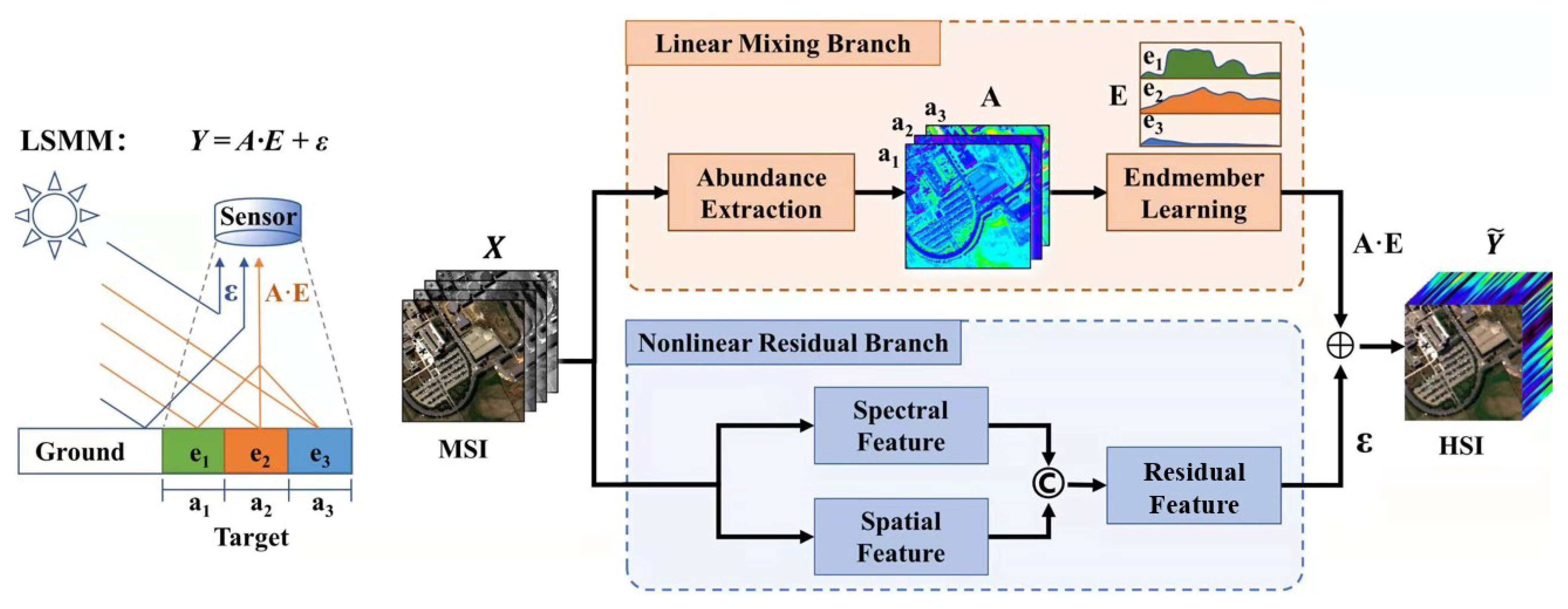
Figure 1. The spectral mixing process and inspired double-branch network structure.
Remotesensing 15 01308 g001
Figure 2. The architecture of a spectral mixing theory-based network. The proposed network consists of a linear mixing branch and a nonlinear residual branch. The linear mixing branch generates rough HSIs as an intermediate result through the abundance extraction module and endmember adaptive learning layer. The nonlinear residual branch extracts nonlinear features from the spatial and spectral dimensions of the multispectral images (MSIs), and maps them to a residual image. Finally, spectral super-resolution (SSR) is achieved by fusing intermediate results and residual images.
Remotesensing 15 01308 g002
Figure 3. Color-combination images of three MSI–HSI datasets employed in the experiment. (a) Indian Pines data. (b) Pavia University data. (c) ZY1-02D data. The MSI–HSI image pair of the highlighted areas in the red rectangle is used for training, and the MSI of the remaining areas is used for testing.
Remotesensing 15 01308 g003
Figure 4. Visualization of SSR results of five methods using Pavia University dataset. Columns 1 to 4 show the absolute error of a single band. Columns 5 and 6 show the overall RMSE and SAM errors for all bands, the highlighted areas in the red rectangle are buildings.
Remotesensing 15 01308 g004
Figure 5. The spectral response function (SRF) of the QuickBird sensor.
Remotesensing 15 01308 g005
Figure 6. Visualization of SSR results of five methods using Indian Pines dataset. Columns 1 to 6 show the absolute error of a single band. Columns 7 and 8 show the overall RMSE and SAM errors for all bands, the highlighted areas in the red rectangle are roads and hay in the 1000 nm. Additionally, the proposed method has a darker blue color in the red box in the RMSE heat maps, indicating superior performance.
Remotesensing 15 01308 g006
Figure 7. Visualization of SSR results of five methods with ZY1-02D dataset. Columns 1 to 4 show the absolute error of a single band. Columns 5 and 6 show the overall RMSE and SAM errors for all bands, the highlighted areas in the red rectangle are river and vegetation.
Remotesensing 15 01308 g007
Figure 8. (ag) shows the endmember spectral curves and corresponding abundance images extracted from the network with the Pavia University dataset. (h) shows invalid abundance and endmember.
Remotesensing 15 01308 g008
Figure 9. (a) Intermediate result generated by linear mixing branch; (b) Residual image generated by nonlinear residual branch; (c) The spectral curve of the red mark in (a,b), and the truth HSI; (d) The residual curve of the red mark in (b).
Remotesensing 15 01308 g009
Figure 10. The variation of PSNR and SAM with endmember number on three datasets.
Remotesensing 15 01308 g010
Figure 11. The variation of PSNR with α and β with the Pavia University dataset. The yellow, green, and blue cubes represent the PSNR of the result when β is 1,10, and 100, respectively.
Remotesensing 15 01308 g011
Table 1. A summary of traditional and deep learning based spectral super-resolution methods.
MethodModelDatasetsCharacteristics and Limitations
Sparse representationArad [18]RGB natural imagesspecific physical significance; limited feature extraction ability
J-SLoL [20]simulated MSIs in small area
(Pavia University; Indian Pines; Jasper Ridge data)
Linear mixingHuang [21]real MSIs in small area
(Hyperion and ALI data)
Deep learningNguyen [22]RGB natural imagespowerful nonlinear mapping ability; few of prior knowledge
Alvaretz-Gila [23]
CanNet [26]
HSCNN+ [27]
HSRnet [17]
HSACS [33]
Galliani [25]
SSRAN [29]
simulated MSIs in small area
(Pavia University; WDCM; Hyperion data)
Table 2. Quantitative results of different methods using Pavia University dataset. “↓” means smaller is better for this index. “↑” means bigger is better for this index.
ModelSAM↓mPSNR↑mSSIM↑RMSE↓ERGAS↓
CanNet2.703341.44230.9812.69657.5656
HSCNN+2.582741.98540.98212.56817.5035
J-SLoL3.197541.25970.97793.09378.9397
SSRAN3.092140.20350.98153.32087.7943
proposed2.440443.33150.98392.25736.4855
Table 3. Quantitative results of different methods using the Indian Pines dataset. “↓” means smaller is better for this index. “↑” means bigger is better for this index.
ModelSAM↓mPSNR↑mSSIM↑RMSE↓ERGAS↓
CanNet2.026445.2240.95922.91743.4896
HSCNN+1.654646.41070.97332.64563.0362
J-SLoL2.140248.06290.96053.10013.5629
SSRAN1.758245.88780.96912.55113.1053
proposed1.706550.36180.97372.54362.8286
Table 4. Quantitative results of different methods on ZY1-02D dataset. “↓” means smaller is better for this index. “↑” means bigger is better for this index.
ModelSAM↓mPSNR↑mSSIM↑RMSE↓ERGAS↓
CanNet1.664744.24580.98362.10654.4467
HSCNN+1.580544.64010.98511.98744.2816
J-SLoL3.244635.01720.88365.91311.8999
SSRAN1.748041.94100.98352.81805.4941
proposed1.560544.82060.98511.97074.1625
Table 5. The test results of single-branch and double-branch with three datasets. “↓” means smaller is better for this index. “↑” means bigger is better for this index.
DatasetModelSAM↓mPSNR↑mSSIM↑RMSE↓ERGAS↓
Pavia universityLinear branch2.551342.76370.98322.4016.8618
Noninear branch2.484142.92990.98342.42567.0207
Double-branch2.440443.33150.98392.25736.4855
Indian pineLinear branch2.203649.65090.96263.17633.5063
Noninear branch1.715450.09540.97282.61552.8442
Double-branch1.706550.36180.97372.54362.8286
ZY1-02DLinear branch1.894441.45190.96582.80465.7678
Noninear branch1.596344.5530.98462.00424.2992
Double-branch1.560544.82060.98511.97074.1625
Table 6. The training time of different methods with the ZY1-02D dataset.
ModelTime Cost (mins)mPSNR
CanNet23.5044.2458
HSCNN+33.0644.6401
J-SLoL41.9235.0172
SSRAN24.1741.9410
proposed28.2544.8206
Disclaimer/Publisher’s Note: The statements, opinions and data contained in all publications are solely those of the individual author(s) and contributor(s) and not of MDPI and/or the editor(s). MDPI and/or the editor(s) disclaim responsibility for any injury to people or property resulting from any ideas, methods, instructions or products referred to in the content.