Article

Unsupervised Cross-Scene Aerial Image Segmentation via Spectral Space Transferring and Pseudo-Label Revising

1
Aerospace Information Research Institute, Chinese Academy of Sciences, Beijing 100190, China
2
Key Laboratory of Network Information System Technology (NIST), Aerospace Information Research Institute, Chinese Academy of Sciences, Beijing 100190, China
3
University of Chinese Academy of Sciences, Beijing 100190, China
4
School of Electronic, Electrical and Communication Engineering, University of Chinese Academy of Sciences, Beijing 100190, China
*
Author to whom correspondence should be addressed.
Remote Sens. 2023, 15(5), 1207; https://doi.org/10.3390/rs15051207
Submission received: 12 January 2023 / Revised: 15 February 2023 / Accepted: 20 February 2023 / Published: 22 February 2023
(This article belongs to the Special Issue Deep Neural Networks for Remote Sensing Scene Classification)

Abstract

:
Unsupervised domain adaptation (UDA) is essential since manually labeling pixel-level annotations is consuming and expensive. Since the domain discrepancies have not been well solved, existing UDA approaches yield poor performance compared with supervised learning approaches. In this paper, we propose a novel sequential learning network (SLNet) for unsupervised cross-scene aerial image segmentation. The whole system is decoupled into two sequential parts—the image translation model and segmentation adaptation model. Specifically, we introduce the spectral space transferring (SST) approach to narrow the visual discrepancy. The high-frequency components between the source images and the translated images can be transferred in the Fourier spectral space for better preserving the important identity and fine-grained details. To further alleviate the distribution discrepancy, an efficient pseudo-label revising (PLR) approach was developed to guide pseudo-label learning via entropy minimization. Without additional parameters, the entropy map works as the adaptive threshold, constantly revising the pseudo labels for the target domain. Furthermore, numerous experiments for single-category and multi-category UDA segmentation demonstrate that our SLNet is the state-of-the-art.

Graphical Abstract

1. Introduction

Aerial image segmentation, which aims to assign a semantic category to each pixel of an image, has various practical applications, including disaster monitoring [1], land-cover planning [2], road extraction [3], building extraction [4], and agricultural valuation [5]. Deep convolutional neural networks (DCNNs) [6,7,8] trained on large-scale remote sensing datasets provide reliable inferential knowledge, greatly promoting recent progress in aerial image semantic segmentation.
However, these data-driven supervised methods [8,9,10,11] need to rely on large amounts of human effort to manually collect and annotate datasets at the pixel level. In addition, a series of mismatches in color texture, spatial layout, and lighting conditions caused by geographical locations, different sensors, etc., also known as the domain shift, cripple the performance of cross-scene aerial image semantic segmentation. As illustrated in Figure 1, we show two discrepancies in unsupervised cross-scene aerial image segmentation. For visual discrepancy, we can clearly see that there is a huge difference in appearance between the source image and the target image, which greatly affects the transfer of knowledge learned from the source domain to the target. For the distribution discrepancy, we present the distribution map for each class by utilizing t-SNE [12], as shown in Figure 1b. Compared with the source-only model (without DA), the distribution map in the target-only model (full-supervision) is more aligned and distinct. Therefore, solving the above discrepancies in the domain shift is the biggest challenge in the cross-scene aerial image segmentation.
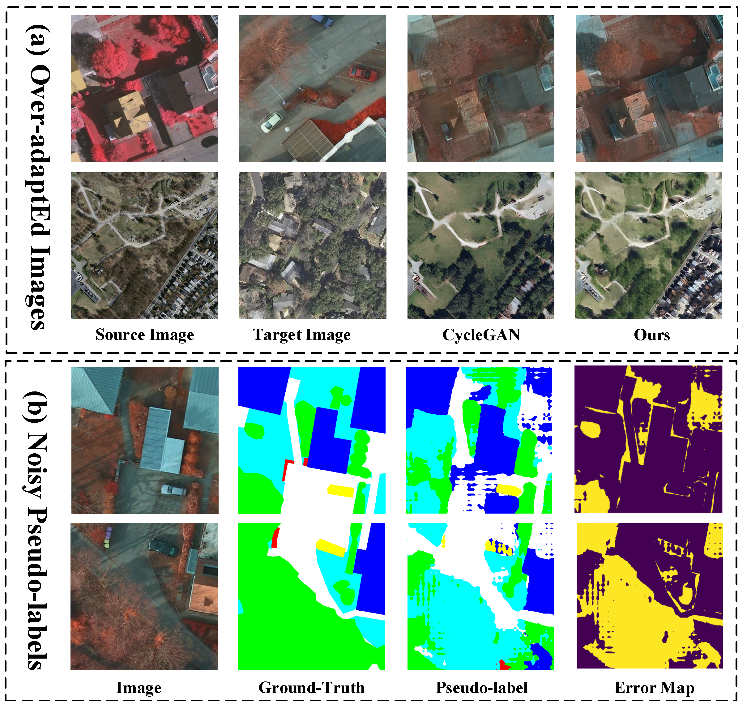
Unsupervised domain adaptation (UDA) is mainly employed to handle the problem of the domain shift, where we focus on the hard case that the datasets in the target domain have no available labels for cross-scene semantic segmentation. Traditionally, UDA methods [13,14,15,16] can be classified into two categories: one focuses on the domain alignment to share the knowledge between the source domain and target domain, and the other is to introduce self-supervised learning (SSL) [17] to mine the domain-specific knowledge of the unlabeled target datasets. For the former, the UDA methods tend to minimize cross-domain discrepancy by learning the metrics with the second moment [14,18,19] and adversarial learning [15,16,20]. Such methods for domain alignment may lead to suboptimal solutions, mainly because the model we ultimately want is suitable for the target domain. Despite the methods [14,15] decreasing the domain shift to a certain extent, it is unnecessary to strictly align the distribution of the source domain and target domain. For example, Figure 2a shows the over-adapted translation results of domain alignment via pixel-level adversarial learning. The translated images in CycleGAN [13] lose critical edges and details related to identity, resulting in suboptimal visual quality. Therefore, ensuring realistic style transfer and fine identity preservation during the image translation process is key. Some recent works [21,22] employ SSL techniques to extract domain-specific knowledge from unlabeled target datasets, thereby improving adaptation to the target domain. However, the pseudo labels are inevitably noisy, resulting in hindrance to subsequent learning. As illustrated in Figure 2b, although a large part of pixels are predicted correctly, pseudo labels still suffer from incorrect predictions due to distribution discrepancy. Recently, many researchers [23,24,25] have focused on ignoring the pseudo labels with low confidence by manually setting the threshold, which is difficult to be determined for different scenes. Different thresholds may be required for the pixels belonging to different target domain scenes, categories, and locations.
In this paper, we propose a novel sequential learning network (SLNet) for unsupervised cross-scene aerial image segmentation. The whole system is decoupled into two separated modules in a sequential learning manner (i.e., “translation-to-segmentation”): spectral-based image translation model and segmentation adaptation model with pseudo-label revising. Specifically, we first introduce the spectral space transferring (SST) module based on the image translation model [13] to generate high-quality translated source domain images. Formally, we maintain the consistency of the high-frequency components of the source image and the translated image in the Fourier spectral space to better preserve the identity and the details. Second, we propose a pseudo-label revising (PLR) approach in our segmentation adaptation model, which is trained on translated source data and target data. Formally, we explicitly incorporate the entropy metric of the prediction results of the two independent classifiers into the training objective function to automatically provide a pixel-level threshold. We adaptively revise the noisy pseudo labels by minimizing the entropy metric, while ensuring a coherent training process. In each iteration, we regard the prediction maps for the target domain as the approximation to the ground truth, and then utilize them to improve the adaptation ability. After many iterations, the shared knowledge across the domain and the domain-specific knowledge can be provided by the pseudo labels to better adapt to the target domain.
In summary, the two models learned in a sequential learning manner stimulate and promote each other, which not only leads to narrowing the domain discrepancies but also can exploit the domain-specific knowledge in the target domain. The main contributions of this paper are summarized as follows:
  • Different from most UDA segmentation methods, we propose a sequential learning system for unsupervised cross-scene aerial image segmentation. The whole system is decoupled into the image translation model and segmentation adaptation model.
  • The spectral space transferring (SST) module is proposed to transfer the high-frequency components between the source image and the translated image, which can better preserve the important identity and fine-grained details.
  • To further alleviate the distribution discrepancy, an efficient pseudo-label revising (PLR) approach was developed to guide pseudo-label learning via entropy minimization. Without additional parameters, the entropy minimization works as the adaptive threshold to constantly revise the pseudo labels for the target domain.

2. Related Works

2.1. Aerial Image Semantic Segmentation

With the acquisition of abundant aerial images and the development of deep learning technologies, large-scale aerial image semantic segmentation (AISS) has led to rapid development. Therefore, numerous CNN-based methods [6,8,26,27,28,29,30] and methods for model explainability [31,32,33] have been applied to the semantic segmentation of aerial images. There are three major challenges in AISS: large scale, pattern diversity, and semantic ambiguity, the latter of which is mainly due to a lack of semantics or the existence of different categories with similar spectral characteristics. To settle the large-scale issue, Tong et al. [26] designed a hybrid land-cover classification algorithm by combining hierarchical segmentation and patch-wise classification to obtain accurate boundary and category data. To solve the pattern diversity issue, ScasNet [27] captured multi-scale contexts in a self-cascaded manner and proposed a residual correction scheme for multi-scale feature fusion. For the third challenge, a lot of work was carried out in succession. S-RA-FCN [6] introduced the spatial relation module and the channel relation module to explicitly aggregate long-range contextual information to produce relation-augmented features. HMANet [28] proposed a hybrid multiple attention network containing class-augmented, class-channel and region shuffle attention to obtain global contextual information from different perspectives. Faced with the complex spectral characteristics of aerial images, DSMFNet [29] introduced the digital surface model (DSM) by four fusion strategies as auxiliary data to improve the performance of similar color regions. In addition, HECR-Net [30] jointly reason the 2D and 3D information by implicitly embedding height information to obtain more discriminative features. Although the above methods have achieved great success, the above methods are supervised by pixel-level labels, which are time-consuming and labor-intensive. In addition, these algorithms often fail on cross-scene datasets due to domain gaps.
To solve the above issues, numerous domain adaptation methods have been proposed for cross-scene aerial image semantic segmentation. GAN-RSDA [34] addressed the style discrepancy issue by adopting generative adversarial networks (GANs) to reduce the domain gaps. ColorMapGAN [35] addressed the spectral distribution shift by presenting a color mapping generative adversarial framework. SRDA-Net [36] explicitly addressed the unsupervised domain adaptation (UDA) for AISS with a different resolution by designing an asymmetric multi-task learning framework, containing segmentation and super-resolution. ScaleNet [37] addressed the cross-scale problem by proposing a scale-aware adversarial learning network to adapt to differences in the scale explicitly. BSANet [38] extracted the features in the wavelet domain and image domain by introducing a bispace adversarial learning strategy to minimize the discrepancy. These GAN-based methods are usually not easy to train and acquire cross-domain shared knowledge, failing to make rational use of the knowledge in the target domain.

2.2. UDA for Semantic Segmentation

In order to rectify domain discrepancy, UDA is applied to transfer knowledge from the source domain to the target domain, so as to achieve better generalization capability. There exists numerous tasks [39,40] that can significantly benefit from UDA, while we mainly focus on the application of UDA in semantic segmentation. The main challenge of UDA for semantic segmentation is the distribution discrepancy of cross-scene data. Therefore, we mainly introduce several common UDA methods to deal with the above challenge in this section.
Domain Alignment aims to learn the shared knowledge across domains to align the data distribution between the target domain and source domain. According to the suggestions of theoretical analysis [41], domain alignment methods can be roughly divided into minimizing the distribution discrepancy by optimizing some divergence [14,18,19] and employing adversarial learning at different levels.
For the former, some discrepancy metrics, such as maximum mean discrepancy (MMD) [19], as well as distance divergences, are adopted to reduce the domain discrepancy. TCA [42] utilizes the MMD criterion to minimize the marginal distributions across domains in the kernel Hilbert space (RKHS) to learn a set of transfer components. JDA [43] expands TCA by jointly matching both the conditional distribution and marginal distribution in a dimension reduction process using PCA to construct robust features. AutoDIAL [44] introduces a domain alignment layer to match the statistics between two domains to reduce the domain shift. Massimiliano et al. [45] extended MMD to the statistical distribution of each layer to appropriately align the distribution of features between the source and target domains. Unfortunately, matching statistics using the first- and second-order moments cannot perform domain alignment well when the distribution does not obey Gaussian.
For the latter, adversarial learning methods are usually based on the GANs, which are composed of generators responsible for generating interested samples and discriminators responsible for determining the authenticity. Adversarial learning often occurs at different levels: image level [15,46,47], the inter-mediate feature level [16,48], and the output space level [20,49]. Image adversarial adaptation mainly refers to unsupervised image-to-image translation, which can be trained with the supervision of unpaired images. Although this strategy independently completes the alignment of marginal distribution, it cannot preserve semantic consistency, which leads to multiple domain invariant representations for suboptimal solutions. Feature adversarial adaptation aims at exploiting the statistical matching of intermediate representation to discover domain-invariant features. At the same time, semantic complexity may bring challenges to adversarial learning. Output adversarial adaptation conducts the cross-domain distribution alignment at the output space to avoid dealing with the high-dimensional feature.
In fact, there is no need to strictly align the distribution as long as the features are well separated. The above methods focusing on domain alignment simply align and capture shared knowledge across domains, but ignore the specific information in the target domain.
Self-supervised learning aims to utilize the generated pseudo labels to improve the adaptation to the target domain, which is also referred to as self-training or self-labeling. As the pseudo labels are inevitably noisy, confidence regularization is employed to explicitly selects prediction maps for training. Common typical methods for acquiring pseudo labels contain handcrafted thresholds with softmax predictions [50,51], class prototypes distance [22,52], clustering [53], and so on. Lee et al. [54] picked up the category with maximum predicted probability as pseudo labels for the unlabeled target dataset, and then trained the network in a supervised fashion. TPN [52] aligns the prototypes of each class between the source and target domain in the embedding space to reduce the distribution discrepancy. BDL [25] leveraged the pseudo labels with high confidence for feature adaptation, where image translation and segmentation adaptation models are learned in a bidirectional learning manner. Zheng and Yang [21] reduced the predicted inconsistency by applying an orthogonal method to learn the domain-specific features. ProDA [22] leveraged the representative prototypes to estimate the likelihood of pseudo labels and align the prototypical assignments. However, the weakness of self-supervision learning is that pseudo labels are inevitably noisy, which can affect subsequent training.
Different from existing works, we decoupled the UDA semantic segmentation into image translation and segmentation adaptation by combining adversarial learning and self-supervised learning methods to capture cross-scene shared knowledge and specific knowledge in the target domain. In addition, instead of using a handcrafted threshold to filter pseudo labels, we use entropy regularization to revise pseudo labels. This framework not only visually eliminates the domain shift across scenes, but also further reduces the feature distribution discrepancy between the source and target domain, which helps us to produce better segmentation performance.

3. Methodology

We first provide an overview, as well as the definition and description of the problem in Section 3.1. To solve the problem, we propose a novel learning framework decoupled into two stages: image translation and domain adaptation segmentation. Specifically, we introduce spectral space transferring (SST) in the first stage (Section 3.2) and pseudo-label revising (PLR) in the second stage (Section 3.3). Finally, Section 3.4 describes the details of loss functions between image translation and segmentation adaptation model.

3.1. Overview

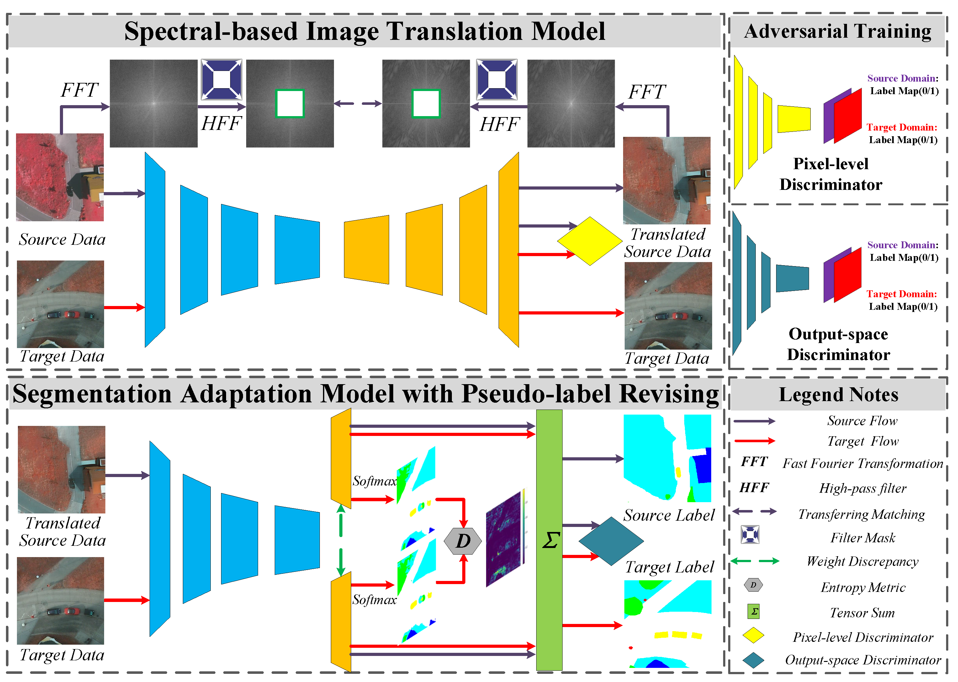
Concretely, given the source images X s = X s i i = 1 M with ground truth labels Y s = Y s i i = 1 M and the target images X t = X t j j = 1 N without segmentation labels Y t = Y t j j = 1 N , we aim to estimate the segmentation adaptation model parameter to minimize the prediction bias to assign category labels Y t for the datasets in the target domain. However, the domain gaps in the visual and feature distribution between the target and source domain bring great challenges for the model to learn transferable knowledge at the same time. In order to respond to the above challenges, we decouple the network into two separated subnetworks inspired by [25,46]. As illustrated in Figure 3, different from complicated and tedious bidirectional learning in [25], we adopt simpler sequential learning, which means that we take the output of the first stage as the input of the second stage. We believe that we can obtain high-quality translated images with good identity preservation in the first stage, so as to avoid issues, such as hard convergence caused by bidirectional learning. The overall structure of the proposed SLNet for UDA semantic segmentation can be illustrated in Figure 4.
First, we obtain the translated images X s = X s i i = 1 M by introducing a spectral-based image translation model IT , which is in charge of unpaired image-to-image translation from source S to target T. The framework is encapsulated into the encoder–decoder structure with nine blocks as a pixel-level discriminator. Such a framework may lose part of the identity details of the source data under the constraint of adversarial loss, which is not conducive to producing high-quality translated images. Therefore, we introduce the spectral space transferring (SST) module on the basis of [13] to preserve high-frequency information representing important details and identity characteristics during training. The purpose of this stage is to minimize pixel-level distribution gaps between the source and target domain.
In the second stage, we input the translated source images X s with Y s , and target images X t into the segmentation adaptation model SA . A feature extractor applies a backbone ResNet-101 [55] to produce a multi-scale hierarchical feature map, which is input to two independent classifiers C 1 and C 2 to generate uncertain prediction results. Moreover, we introduce self-supervised learning (SSL) to make full use of the knowledge of the unlabeled target domain, and add the pseudo-label revising (PLR) module to automatically set the threshold to correct pseudo-label learning. Different from the source flow, we employ the widely used JS-divergence of two predictions as the uncertain entropy map to revise the learning from noisy pseudo labels in the target flow. In addition, we also performed distribution alignment at the output space level. To make a summary, we first minimize the distribution discrepancy between the source domain and the target domain at different levels, and then leverage the knowledge of the unlabeled data by modifying pseudo-label learning, with the ultimate goal of reducing the distribution discrepancy between the source and target domain.

3.2. Spectral Space Transferring

In order to regulate the momentous structural characteristics during the process of image translation, we propose an image translation framework based on spectral space transferring. The model is inspired by digital signal processing [56]. As illustrated in Figure 5, we decompose the original image into low-frequency and high-frequency components via the fast Fourier transform (FFT) algorithm [57]. Intuitively, the high-frequency component seizes the information such as sharp edges and minute details, while the low-frequency component corresponds to the color and style representation. Our key idea is to maintain high-frequency consistency across source-domain images and the translated source-domain images in the Fourier spectral space. More specifically, we first map X s into spectral space through the FFT algorithm [57].
F ( X s ) ( m , n ) = h = 0 H 1 w = 0 W 1 X s ( h , w ) e 2 π i m h H + n w W , i 2 = 1
in which, m [ 0 , H 1 ] , n [ 0 , W 1 ] . It can be clearly seen from Equation (1) that each point in F ( X s ) ( m , n ) gathers the global information of all pixels in the frequency spectral space. Most notably, we convert color images to grayscale images to erasure color and lighting information irrelevant to details and sharp edges of objects. For easy implementation of high pass filters, we convert the spectrum F r of FFT to the real number and move the zero-frequency component to the center of the spectrum without losing any information.
F r ( X s ) = Re F ( X s ) 2 + Im F ( X s ) 2
where Re F ( X s ) and Im F ( X s ) indicate the real part and the imaginary part of F ( X s ) ( m , n ) separately. Then, the low-frequency part of the spectrum F r is covered by a high pass filter, while the high-frequency component is retained. We denote with M γ a filter mask (white square in Figure 3), where the value in the center region is zero, and the value of the other region is one. Here, we suppose the center of the image is (0, 0).
F r h ( X s ) = F r ( X s ) · M γ
M γ ( h , w ) = 0 , ( h , w ) [ γ H : γ H , γ W : γ W ] 1 , o t h e r w i s e
The selection of super parameters γ is independent of the size or resolution of the input X s , which is due to the fact that γ is not measured in pixels. We reveal the effect choices of γ on UDA segmentation in Section 4.4.3. The process of spectral space transferring can be formulated as:
L s s t = E X s S [ F r h ( X s ) F r h ( X s ) s m o o t h ]
where · s m o o t h denotes smooth L 1 normal. This loss restrains the high-frequency components between the generated image and the source image to be consistent in the spectral space, so as to better preserve the identity.

3.3. Pseudo-Label Revising

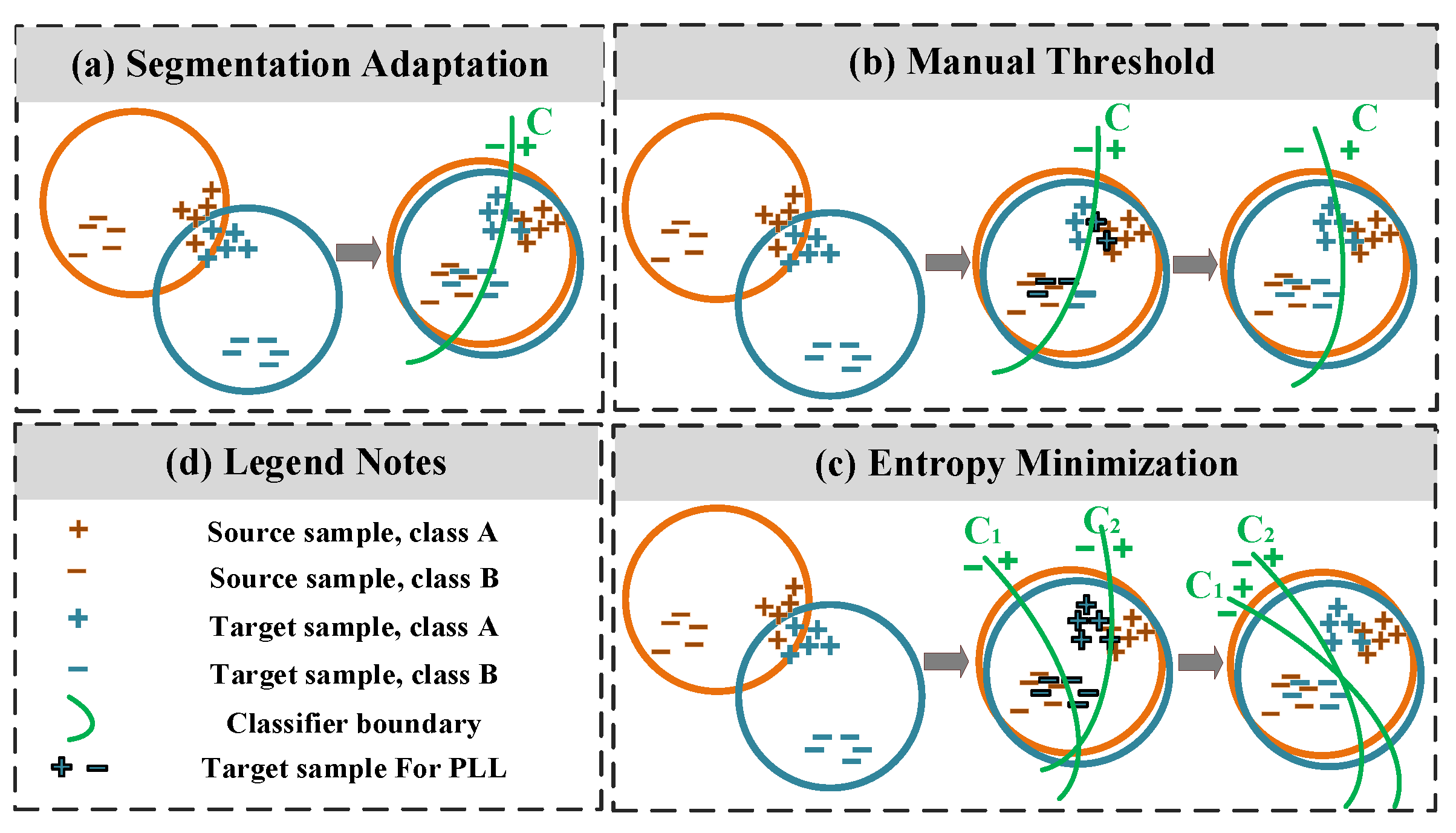
The spectral-based image translation model learns the knowledge shared by the target domain and the source domain but ignores the specific knowledge of the target domain. Recently, some work has introduced self-supervised learning ( S S L ) for pseudo-label learning ( P L L ) of the target domain. In this paper, SSL is equivalent to PLL. We employ the illustration (shown in Figure 6a,b) to explicate the tenet of this process. The specific approach generally includes two steps. First, X s with ground truth labels Y s and X t are input into the segmentation adaptation model SA . The first step is to generate the pseudo-label Y t ^ for the unlabeled X t , where the objective can be formulated as follows:
L a d v ( X s , X t ) = E X t T [ D SA ( X t ) ] + E X s S [ 1 D SA ( X s ) ]
L s e g ( X s , Y s ) = E X s S [ Y s j log F ( X s j | Θ s ) ]
L SSL 1 = α a L a d v ( X s , X t ) + α s L s e g ( X s , Y s )
where D SA indicates the discriminator in the segmentation adaptation (SA) model and L a d v is the adversarial loss to reduce the distribution discrepancy between the source domain and target domain at the output space level. L s e g measures the segmentation accuracy for the translated source images X s . Note that α a and α s are taken as 0.001 and 1, respectively. Then, some pseudo labels Y t ^ can be obtained with high confidence based on the prediction probability. The second step of self-supervised learning is to minimize the prediction bias using X s with ground truth labels Y s and X t , with pseudo labels Y t ^ , where the objective can be formulated as follows:
L s e g ( X t , Y t ^ ) = E X t T [ Y t ^ j log F ( X t j | Θ t ) ]
L SSL 2 = α a L a d v ( X s , X t ) + α s L s e g ( X s , Y s ) + α t L s e g ( X t , Y t ^ )
where α a , α s , and α t are utilized as weighting factors, with values of 0.001, 1, and 1, respectively. The combination of SSL and adversarial learning cannot only reduce the distribution discrepancy but also predict the correct pseudo labels for the target domain. However, there is an inherent problem that pseudo labels inevitably contain noise, which can largely harm the training. The main reason is that setting the threshold manually only utilizes pseudo labels with high confidence and ignore labels with low confidence.
To correct the label noise during self-supervised learning, we propose a pseudo-label revising module, which can learn an automatic threshold from the uncertain entropy map to constrain the generation of pseudo labels. Inspired by [58], we try our best to make two classifiers C 1 and C 2 have different parameters by minimizing the cosine similarity of the weights as follows:
D C S = w 1 · w 2 w 2 w 2
where w 1 and w 2 denote the weights of classifiers C 1 and C 2 separately. Here, D C S helps us to leads to the discrepancy of C 1 and C 2 , which is beneficial to the generation of uncertainty entropy map. As shown in Figure 4, we employ the widely used JS-divergence of C 1 and C 2 classifier outputs as the uncertain entropy map to guide the learning from noisy pseudo labels in the target flow.
D J S = 1 2 E [ F 1 ( X t j | Θ t ) log ( F 1 ( X t j | Θ t ) F 2 ( X t j | Θ t ) ) ] + 1 2 E [ F 2 ( X t j | Θ t ) log ( F 2 ( X t j | Θ t ) F 1 ( X t j | Θ t ) ) ]
where F 1 ( X t j | Θ t ) and F 2 ( X t j | Θ t ) indicate the probability distribution of X t j generated by the classifiers C 1 and C 2 , respectively. It is worth noting that the more different the distributions provided by the two classifiers are, the larger their entropy values. Compared with classical pseudo-label learning, the proposed pseudo-label revising based on entropy minimization (shown in Figure 6c) utilizes the discrepancy entropy map as the automatic threshold to guide the PLL process.

3.4. Training Objective

In the previous part, we introduced the sequential learning framework for unsupervised multi-task learning, including image translation and UDA semantic segmentation. We explicate the training procedure and the details of the objective (presented in Algorithm 1) in this section.
Algorithm 1 Training process of the proposed method.
  • Input: The source domain dataset X s with ground truth Y s ; the target domain dataset X t ; the iteration number K.
  • Output: The segmentation adaptation model parameter Θ t .
1:
Generate high-quality translated source dataset X s by IT
2:
Train the source-domain parameter Θ s according to Equation (8), and generate pseudo-label Y t ^
3:
Initialize Θ t = Θ s
4:
for k → 1 to K do
5:
    Input X t to SA , enforce weight discrepancy of the two classifiers C 1 and C 2 by cosine similarity D C S
6:
    Utilize the JS-divergence D J S to measure the entropy map
7:
    In the target flow, combine the conventional objective L s e g ( X t , Y t ^ ) , D C S , and D J S as follows:
L p l r ^ ( X t , Y t ^ ) = e D J S [ L s e g ( X t , Y t ^ ) + D C S ] + D J S
8:
    Combine the objective in the source and target flow, as well as the adversarial objective to update the Θ t .
9:
end for
When the spectral-based image translation IT model is learned, the objective contains two components: the loss L g a n and the objective function for SST L s s t .
L g a n ( X s , X t ) = E X s S [ D IT ( X s ) ] + E X t T [ 1 D IT ( X t ) ]
L g a n ( X t , X s ) = E X t T [ D IT ( X t ) ] + E X s S [ 1 D IT ( X s ) ]
L IT = α g a n [ L g a n ( X s , X t ) + L g a n ( X t , X s ) ] + α s s t L s s t
where D IT indicates the discriminator in the image translation (IT) model and the GAN loss L g a n enforces a similar distribution between the source and target domain. The spectral space transferring (SSL) loss L s s t is utilized for better identity preservation ( s s ) while realizing realistic style transfer ( s t ). α g a n and α s s t represent the weights of their loss functions, which are taken as 1 and 0.5 , respectively, in the work.
While the segmentation adaptation SA model is trained, we proposed the pseudo-label revising (PLR) module to guide more effective learning from noisy pseudo labels. As shown in Algorithm 1, we modify the SSL objective function in the target flow on the basis of Equation (10), which is also the difference between our proposed pseudo-label revising and the classical pseudo-label learning (illustrated in Figure 6). It is worth noting that we do not always intend to minimize L s e g ( X t , Y t ^ ) and D C S . In other words, when the entropy metric D J S has received one larger value, we expect the network to stop punishing L s e g ( X t , Y t ^ ) and D C S , and vice versa. Therefore, we introduce a coefficient e D J S as a trade-off. Combined with the objective in the source flow and the adversarial objective, the modified objective function can be formulated as:
L SA = α a L a d v ( X s , X t ) + α s L s e g ( X s , Y s ) + α t L p l r ^ ( X t , Y t ^ )

4. Experiments

4.1. Datasets

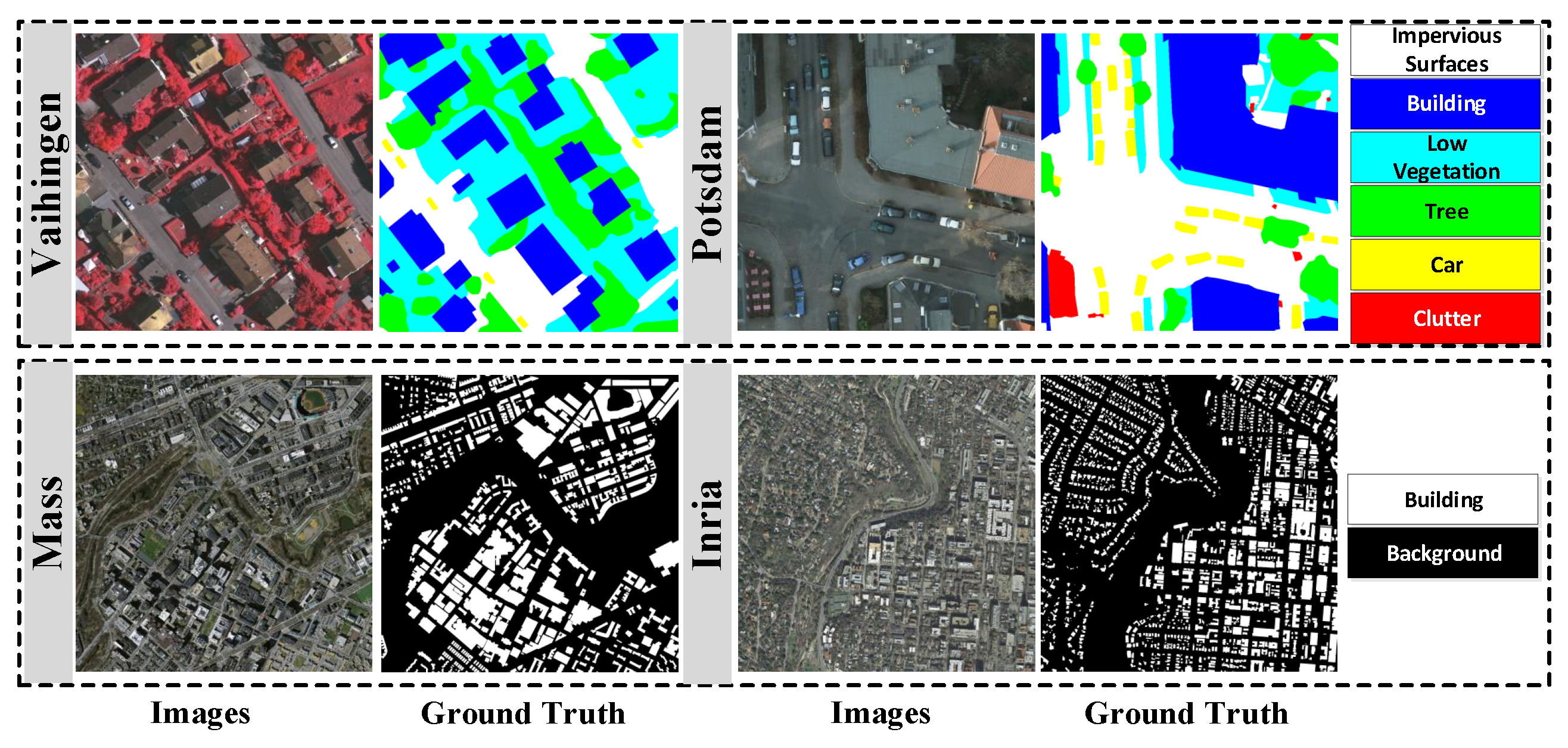
In order to demonstrate the effectiveness of the proposed framework for unsupervised cross-scene domain adaptation, we use the following two pairs of UDA datasets for single-category and multi-category semantic segmentation, respectively, as illustrated in Figure 7.
Mass–Inria: single-category UDA semantic segmentation.
  • The Massachusetts building dataset [59] embodies 151 patches of the Boston area consisting of aerial images with a spatial resolution of 1 m/pixel and a size of 1500 × 1500 pixels. The entire dataset covers about 340 square kilometers, in which 137 tiles are selected as training sets, 10 tiles are selected as testing sets, and the remaining 4 tiles are selected to validate the proposed network. For each image in the dataset, the corresponding ground-truth labels are provided, which contain two categories: building and background.
  • The Inria aerial image labeling dataset [60] consists of 360 RGB ortho-rectified aerial images with a resolution of 5000 × 5000 pixels and a spatial resolution of 0.3 m/pixel. Following the previous work [36], we arrange images 6–36 for training and images 1–5 for validation. The corresponding ground-truth labels contain two categories: building and background are provided.
Vaih-Pots: multi-category UDA semantic segmentation
  • ISPRS Vaihingen 2D Semantic Labeling Challenge dataset contains 33 patches, where the training set embodies 16 tiles and the remaining 17 tiles are selected to test the proposed method. Each aerial image contains the corresponding true orthophoto (TOP) and semantic label, which has an average size of 2494 × 2064 pixels and a ground sampling distance of 9cm. The corresponding ground-truth labels contain six categories: impervious surface, building, low vegetation, tree, car, and clutter/background.
  • ISPRS Potsdam 2D semantic labeling challenge dataset involves 38 patches, in which 24 images are used for training and the validation set contains 14 tiles. Each aerial image has an average size of 6000 × 6000 pixels and a ground sampling distance of 5 cm.

4.2. Implementation Details

In our experiments, the whole framework is implemented with the PyTorch platform on four Tesla P100 graphics processing units. In the first stage, we choose to employ CycleGAN [13] with nine blocks as our image translation IT model and add the spectral space transferring module. Limited to GPU memory, the images are cropped into 452 × 452 by applying random operations. When training the spectral-based image translation model, the initial learning rate is set to 2 × 10 4 , and decreased with the ‘lambda’ learning rate policy. The whole IT network is optimized with the ‘Adam’ optimizer for 20 epochs. In the second stage, the DeepLab V2 [11] with ResNet-101 [55] pre-trained on the ImageNet dataset [61] is adopted as our segmentation adaptation SA model. Following [62], we introduce an output space discriminator with five convolution layers, in which the channel numbers in each layer are 64 , 128 , 256 , 512 , 1 , respectively. When training the SA network, we employ a stochastic gradient descent (SGD) [63] with weight decay 0.0005 and momentum 0.9 as the optimizer. The initial learning rate is 2.5 × 10 4 , and multiplied by 1 ( i t e r m a x _ i t e r ) p o w e r with p o w e r = 0.9 . In addition, the initial learning rate in the output space discriminator is set to 1 × 10 4 with a momentum of 0.99. Following the previous work [8,30], we comprehensively validate the performance of the model by a total of two common evaluation metrics: Intersection over union (IoU) and F 1 score. It is noteworthy that we count the metrics for all categories except clutter in the multi-category UDA semantic segmentation.

4.3. Experimental Results

4.3.1. Results on Single-Category UDA Semantic Segmentation

As reported in Table 1, we compare the results of the proposed SLNet with the other state-of-the-art, from Mass to Inria and Inria to Mass, respectively, to verify the effectiveness of single-category UDA semantic segmentation. Bold values represent the best score in the column.
From Mass to Inria, our SLNet achieves the ascendant result with mIoU of 57.32%, which outperforms that of BDL (mIoU of 54.16%) [25], SRDA-Net (mIoU of 52.86%) [36] and so on. It is worth noting that our SLNet enables a boost over the source-only model (without domain adaptation) by 26.53% in mIoU, while underperforming the target-only model (supervised) by 26.17% in mIoU. From Inria to Mass, our SLNet achieves a result of 51.16% in mIoU, which brings great improvement compared with the source-only model. Both experimental results verify the effectiveness of our SLNet for single-category UDA semantic segmentation.
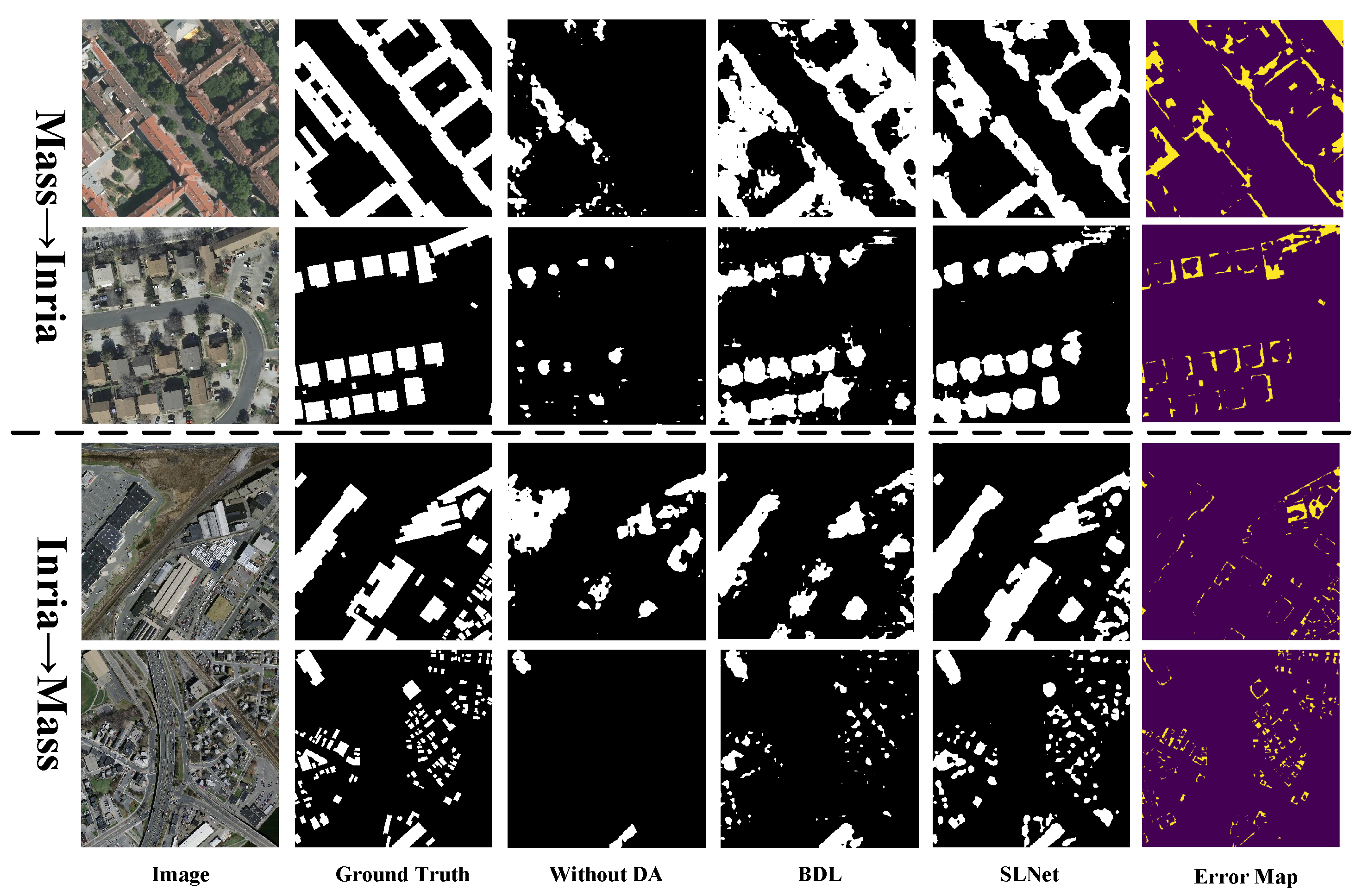
In order to further analyze the UDA semantic segmentation performance, we conducted a visual analysis of the experimental results based on the Mass and Inria dataset, as illustrated in Figure 8. Here, the visualization of the first two lines are from Mass to Inria and the last two lines are from Inria to Mass. Moreover, from the first column to the last column are images, ground truth, the results without DA, the results by applying BDL, our results, and the error map, respectively. It can be clearly seen that compared with the model without DA and BDL [25], our segmentation results have more accurate prediction and fewer errors. Benefiting from sequential learning, including the image translation model with spectral space transferring (SST) and segmentation adaptation model with pseudo-label revising (PLR), we achieved the best results for single-category UDA semantic segmentation.

4.3.2. Results on Multi-Category UDA Semantic Segmentation

Different from single-category UDA semantic segmentation, multi-category UDA semantic segmentation is more challenging due to domain gaps in spectral texture and category distribution of multiple categories. Similarly, we perform the comparison on two tasks (Vaihingen ⇒ Potsdam and Potsdam ⇒ Vaihingen) to verify the effectiveness of our SLNet.
From Vaihingen to Potsdam, we report the quantitative results in Table 2, where the proposed SLNet with ResNet-101 [55] is compared with the other state-of-the-art. We observe that our SLNet achieves the best with mIoU of 62.58%, and mean F 1 of 75.85%. Most of the work only focuses on feature alignment from the source domain to the target domain by employing different adversarial losses, where the knowledge of the unlabeled target domain is not fully utilized. The best performance in BDL [25] is still 7.11% worse in mIoU than our SLNet. Compared with BDL [25], we also introduce the image translation model followed by the segmentation adaptation model to further reduce the domain gaps, but the multi-task learning architecture is different. Compared with complex bidirectional learning, sequential learning is more convenient for training and convergence. Meanwhile, there is still a certain gap between the results of our SLNet and the target-only model, which needs further exploration.
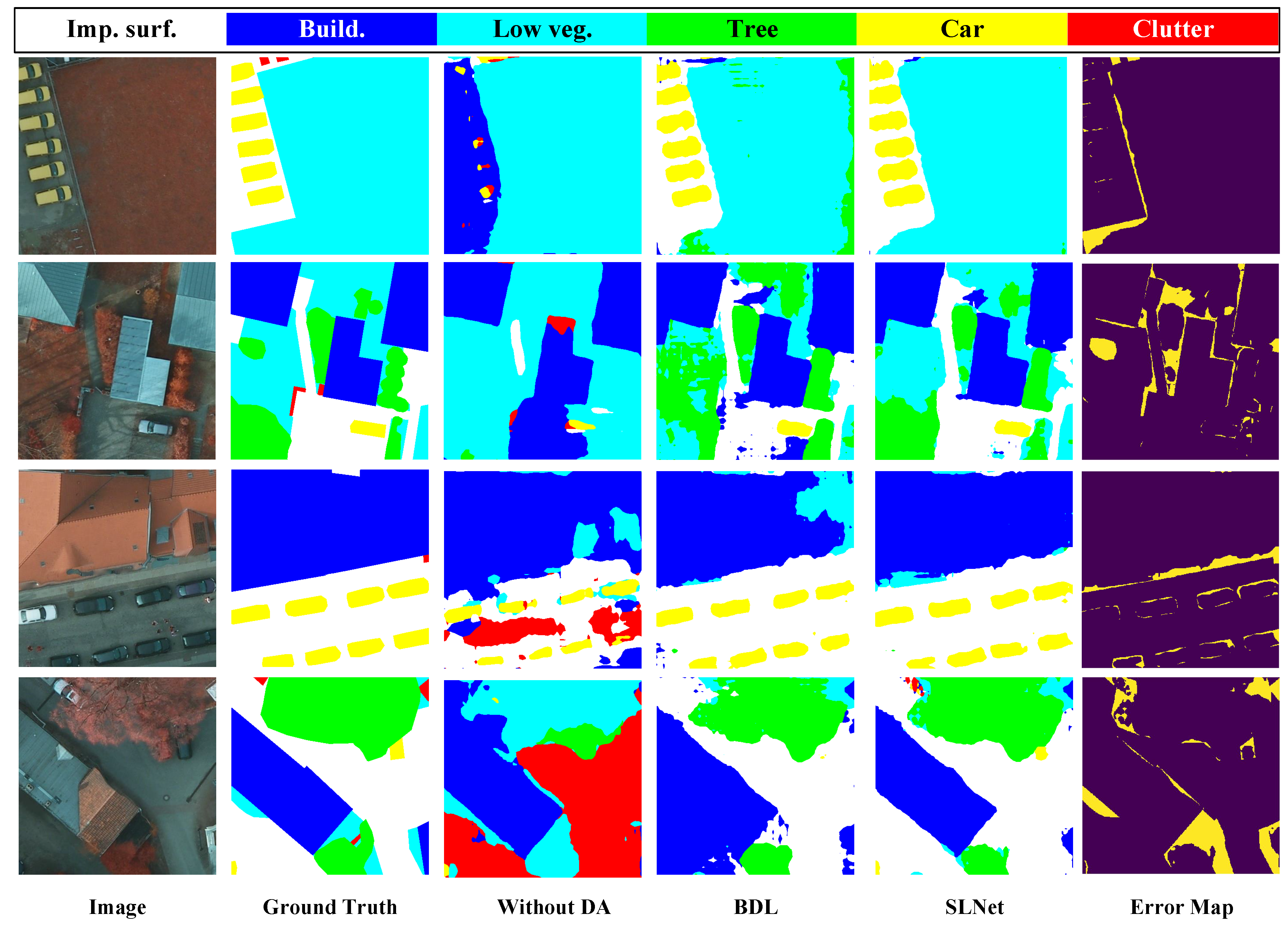
To more vividly show the effect of the algorithm, Figure 9 showcases four typical UDA segmentation results, where the segmentation results of the model without DA, BDL [25], our SLNet, and the error maps are visualized. Through visualizations in Figure 9, we can find that our SLNet obtains more accurate segmentation maps with a novel proposed sequential learning method.
From Potsdam to Vaihingen, we compare the quantitative performance between our method and the state-of-the-art methods. As presented in Table 3, our SLNet yields a considerable amplification of 62.71% and 76.42% in mIoU and mean F 1 , respectively. We also list the quantitative performance for the five categories for a fair comparison. Our SLNet decouples one task into two subtasks to narrow domain discrepancy from pixel-level and output space, respectively. Compared with the most advanced algorithm [66], we enable a boost of 4.42% and 6.36% in mIoU and mean F 1 . BDL [25] is very similar to our work, but the low prediction confidence for the category, such as ’Low vegetation’ and ’Car’ will lead to the poor prediction of pseudo labels, which can affect self-supervised learning. In addition, we conducted qualitative and visual analyses of the experimental results, as illustrated in Figure 10. Note that, we chose 452 × 452 patches for the best visualization. Moreover, benefiting from the image translation model with spectral space transferring (SST) and the segmentation adaptation model with pseudo-label revising (PLR), the proposed SLNet predicts the finer segmentation maps for multi-category UDA semantic segmentation.

4.4. Ablation Analysis

In this section, we carry out extensive ablation experiments ( V a i h i n g e n P o t s d a m ) to verify the effectiveness of sequential learning and the key modules of our model. Note that we take Vaihingen as the source domain dataset and Potsdam as the target domain dataset.

4.4.1. Discussion

The advantages of the proposed sequential learning network (SLNet) can be summarized as follows: First, the image translation (IT) model and segmentation adaptation (SA) model are combined together in a sequential way, which helps decrease both visual and distribution domain discrepancy. Most prior UDA methods focus on only one of these two discrepancies, whilst maintaining a standard implementation of the other. Second, different from CycleGAN [13], the proposed spectral space transferring (SST) module ensures the source images and the translated images share a similar high-frequency spectrum, which represents the important details and identity characteristics. Therefore, our image translation model achieves realistic style transfer and preserves detailed information to generate high-quality translated images. Third, the proposed pseudo-label revising based on entropy minimization does not need to set the thresholds manually but can provide adaptive thresholds for different locations. When the entropy value is low, the model focuses on the prediction bias term to learn from pseudo labels; when the entropy value is high, the model is prone to ignoring the prediction bias term to skip noisy pseudo labels.

4.4.2. Analysis of Network Settings

We first explain the symbols used in the ablation experiment to describe our stepwise experiment. Here, A 0 represents the initial network without domain adaptation, where only source domain data are involved in training. A 1 refers to the output space adversarial learning network trained with source and target domain datasets. Moreover, A 2 is to add an auxiliary classifier on the basis of A 1 to measure the uncertainty entropy map of prediction. C indicates that we utilize CycleGAN [13] as the image translation model. T indicates our proposed spectral-based image translation model, which is in charge of producing high-quality translation source domain images. For A 0 ( T ) , A 1 ( T ) , and A 2 ( T ) , the adaptation network is trained based on the translated source and target dataset. In addition, ( [ A 2 ] k ( T ) , k = 1 , 2 , 3 , ) indicates employing pseudo-label revising on the basis of A 2 ( T ) , where k represents the number of iterations.
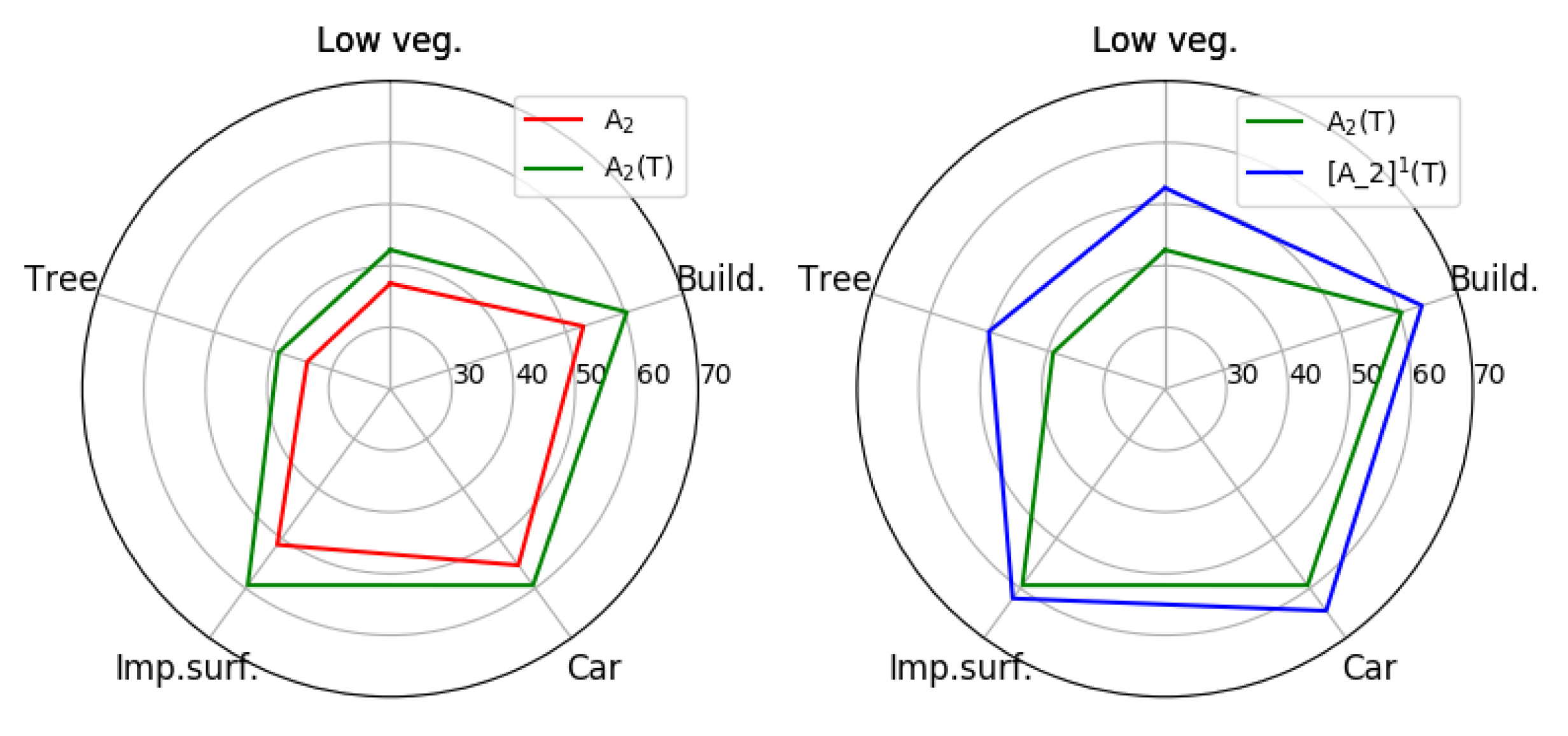
As reported in Table 4, A 0 serves the lower boundary as the baseline, and the middle eight lines show the performance of the method without SSL. A 0 ( C ) outbalances the baseline by 24.12% in mIoU. An interesting phenomenon is that A 1 , A 2 , and A 0 ( T ) enable a similar boost over the baseline by about 28% in mIoU. Compared with the A 0 ( C ) , A 1 ( C ) , and A 2 ( C ) , our proposed spectral-based image translation model, respectively, brings 3.88%, 2.13%, and 1.36% improvement in mIoU, which shows the advantages of SST. It also implies that the image translation and segmentation adaptation model can work independently to reduce domain gaps, and when combined with sequential learning, they can complement each other through an iteration. In addition, we further present the performance improvement of multiple categories on the left side of Figure 11 to verify the effectiveness of the proposed spectral-based image translation model.
We further prove that the revising of SSL can make full use of the knowledge of the unlabeled target domain to improve the adaptation ability. Here, we provide the results through three iterations based on Algorithm 1. When the model A 2 ( T ) is updated to [ A 2 ] 1 ( T ) with pseudo-label revising through one iteration, mIoU can be improved by 6.46%. We attribute this to that SSL with pseudo-label revising (PLR) can utilize the knowledge of the aligned data between the target domain and the source domain, and further guide the remaining data to align. At the same time, we visualized the performance gains of all categories from the A 2 ( T ) to [ A 2 ] 1 ( T ) model on the right side of Figure 11. The largest performance improvement was observed in the category with an mIoU score below 50%. This indicates that our PLR module mitigates the negative impact of low confidence on SSL to a certain extent.
As the number of iterations increases, we enable the automatic threshold to guide the pseudo-label learning by estimating the entropy map, when K = 2 , a large improvement can be obtained from [ A 2 ] 1 ( T ) to [ A 2 ] 2 ( T ) , where mIoU increased by 3.95%. It indicates that more pseudo labels can be utilized to enhance the model’s adaptability. However, the learning of the segmentation adaptive model will be converged with the increase of K . As shown in Table 4, the [ A 2 ] 3 ( T ) model underperforms the [ A 2 ] 2 ( T ) model by 2.34% in mIoU, which may suggest that K = 2 is a good choice. Through the above ablation experiments, we can further confirm that the segmentation adaptation model can give more confident predictions as we continue to reduce domain gaps and modify pseudo-label learning.

4.4.3. Effect of Spectral Space Transferring

In order to verify the effectiveness of the proposed spectral space transferring (SST) module, we report the quantitative results in Table 5. In this section, we take method A 2 without the image translation model as the baseline. Note that we train CycleGAN [13] as our image translation model when γ = 0 . When γ is greater than 0, we introduce the SST module to preserve the frequency information, which represents the important details and identity characteristics during training.
When γ equals 0, the method A 2 ( T ) yields an amplification of 2.01% in mIoU, which indicates that the image translation model can indeed reduce the domain discrepancy in the visual space. In addition, we find in Table 5 that when γ is 0.15 and 0.10, methods A 2 ( T ) and [ A 2 ] 1 ( T ) achieve the best performance, respectively. Theoretically, with the increase of γ , we can preserve much of the high-frequency information to restore the details. However, generous experiments show that when γ is greater than 0.10, our experimental performance is less sensitive to its selection.
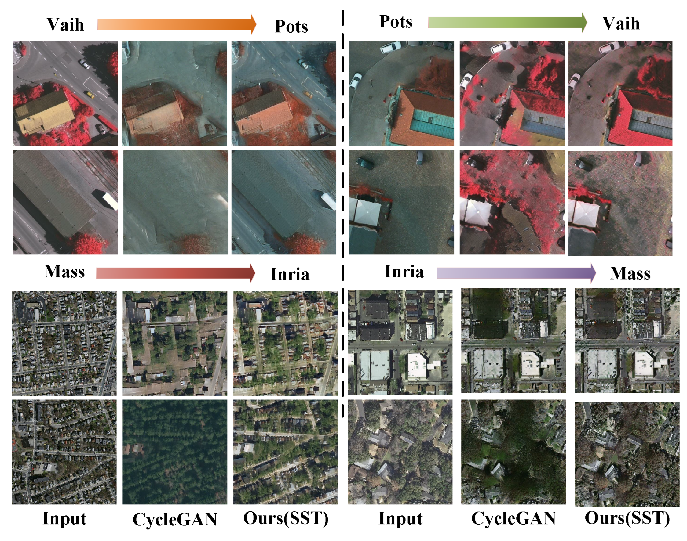
In the case of qualitative analysis, we compare the visualization results between CycleGAN [13] and our spectral-based image translation model, as illustrated in Figure 12. The first two lines belong to multi-category image domain adaptation, where CycleGAN [13] often loses some original details and over-adapts to the reference domain. For example, in the process of image translation from Vaihingen to Potsdam, cars are ignored on the first line and the second line loses the boundary of the building, resulting in poor visual quality. In the process of image translation from Mass to Inria, we find buildings are predicted to be ’other’ due to over-adaptation to the reference domain, and so on. Benefiting from the preservation of high-frequency information during the process of image translation, we can better preserve the identity details while conducting realistic image translation.

4.4.4. Effect of Pseudo-Label Revising

Pseudo-label learning can make use of the knowledge of the unlabeled target domain, but at the same time, it inevitably leads to a lot of noisy information. The classical pseudo-label learning selects pseudo labels with high confidence to participate in training by the handcrafted threshold, which solves the noise problem to a certain extent. However, the threshold is often hard to determine, and the data with low confidence cannot be utilized. In this section, we conduct large quantities of experiments to analyze the effectiveness of the pseudo-label revising module from the following two aspects.
Entropy Minimization vs. Manual Threshold.
As illustrated in Figure 6, we compare the diagram of the classical pseudo-label learning and our pseudo-label revising. The former is based on the manual threshold, while the latter is based on entropy minimization. Here, we report the performance comparison between different manual thresholds and entropy minimization from Vaihingen to Potsdam in Table 6. We can find that the best performance of classical pseudo-label learning based on the manual threshold setting of 0.85 is 56.42% in mIoU, which is 4.25% more than A 2 ( T ) . Compared with the manual threshold method, our method [ A 2 ] 1 ( T ) can reach 58.63% mIoU with a 2.21% increment. This is mainly because that entropy minimization works as the automatic threshold, which constantly revises the corresponding pseudo labels for different categories of pixels. More specifically, the proposed model tends to revise pseudo labels for locations with small entropy to maximize the use of knowledge in the target domain, and is prone to ignoring the pseudo labels for locations with large entropy to minimize the negative impact of noisy pseudo labels.
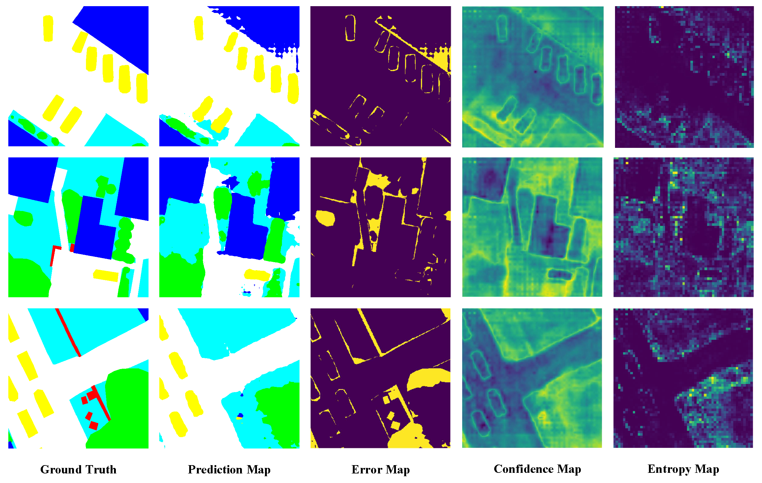
In addition, we visualize the discrepancy between the confidence map and error map to further verify the effectiveness of entropy minimization. As illustrated in Figure 13, there are extensive overlapping highlights between the entropy map and error map, which also indicates that the areas with large entropy in the pseudo labels are often the areas with wrong predictions. Nevertheless, the highlighted areas of the confidence map are usually concentrated on the boundaries of different classes, which does not provide effective clues for uncertain predictions.
Effect of Metric Functions. There are many metric functions to measure the discrepancy of sample distribution, such as maximum mean discrepancy (MMD) [67], KL-divergence, JS-divergence, and so on. Here, we carry out several groups of experiments to compare common metric functions, and the experimental results are reported in Table 7. Compared with the first two functions, we achieved the best performance of 58.63% mIoU by adopting JS-divergence. The reasons are mainly attributed to the following two aspects. On the one hand, MMD [67] focuses on the distribution discrepancy of prediction data and relies on certain prior knowledge (Gaussian kernel function), which is not conducive to the learning and convergence of the network. On the other hand, the two classifiers in this work ( C 1 and C 2 ) are not divided into the main classifier and the auxiliary classifier, so compared with KL-divergence, JS-divergence with symmetry is more suitable for us to measure entropy to guide pseudo-label learning.

5. Conclusions

In this article, a unified sequential learning system (decoupled into the image translation model and segmentation adaptation model) was established to capture domain-shared and domain-specific knowledge for unsupervised cross-scene aerial image segmentation. For narrowing the visual discrepancy, the spectral-based image translation model directly transfers high-frequency components in the Fourier spectral space for better preserving the identity structure. For alleviating the distribution discrepancy, we explicitly incorporate the entropy metric of the prediction results of the two independent classifiers into the training objective function to automatically provide pixel-level threshold. Without additional parameters, we adaptively revise the noisy pseudo labels by minimizing the entropy metric, while ensuring a coherent training process. Such a framework in a sequential learning manner cannot only lead to narrowing the domain discrepancies but can also exploit the domain-specific knowledge in the target domain. Furthermore, the experimental results for single-category and multi-category UDA segmentation demonstrate that our method is better than state-of-the-art UDA segmentation methods.

Author Contributions

Conceptualization, W.L.; methodology, W.L.; software, W.L.; validation, W.L., W.Z., X.S. and Z.G.; formal analysis, W.L. and W.Z.; writing—original draft preparation, W.L.; writing—review and editing, W.L., W.Z., X.S. and Z.G.; visualization, W.L.; supervision W.Z.and X.S.; project administration, W.Z. and X.S.; funding acquisition, W.Z. and X.S. All authors have read and agreed to the published version of the manuscript.

Funding

This research was funded by the National Natural Science Foundation of China under Grants 62171436.

Data Availability Statement

The experiments in this article are based on open source data sets, and no new data is created.

Acknowledgments

The authors thank the staff of the “Remote Sensing” Editorial Office for their support in helping to make the publication of this Special Issue a success.

Conflicts of Interest

The authors declare no conflict of interest.

References

  1. Stewart, I.D.; Oke, T.R. Local climate zones for urban temperature studies. Bull. Am. Meteorol. Soc. 2012, 93, 1879–1900. [Google Scholar] [CrossRef]
  2. Matikainen, L.; Karila, K. Segment-based land cover mapping of a suburban area—Comparison of high-resolution remotely sensed datasets using classification trees and test field points. Remote Sens. 2011, 3, 1777–1804. [Google Scholar] [CrossRef] [Green Version]
  3. Maboudi, M.; Amini, J.; Malihi, S.; Hahn, M. Integrating fuzzy object based image analysis and ant colony optimization for road extraction from remotely sensed images. ISPRS J. Photogramm. Remote Sens. 2018, 138, 151–163. [Google Scholar] [CrossRef]
  4. Jin, X.; Davis, C.H. Automated building extraction from high-resolution satellite imagery in urban areas using structural, contextual, and spectral information. EURASIP J. Adv. Signal Process. 2005, 2005, 745309. [Google Scholar] [CrossRef] [Green Version]
  5. Hamuda, E.; Glavin, M.; Jones, E. A survey of image processing techniques for plant extraction and segmentation in the field. Comput. Electron. Agric. 2016, 125, 184–199. [Google Scholar] [CrossRef]
  6. Mou, L.; Hua, Y.; Zhu, X.X. Relation matters: Relational context-aware fully convolutional network for semantic segmentation of high-resolution aerial images. IEEE Trans. Geosci. Remote Sens. 2020, 58, 7557–7569. [Google Scholar] [CrossRef]
  7. Hua, Y.; Mou, L.; Zhu, X.X. Recurrently exploring class-wise attention in a hybrid convolutional and bidirectional lstm network for multi-label aerial image classification. ISPRS J. Photogramm. Remote Sens. 2019, 149, 188–199. [Google Scholar] [CrossRef]
  8. Liu, W.; Sun, X.; Zhang, W.; Guo, Z.; Fu, K. Associatively segmenting semantics and estimating height from monocular remote-sensing imagery. IEEE Trans. Geosci. Remote Sens. 2022, 60, 5624317. [Google Scholar] [CrossRef]
  9. Zhao, H.; Shi, J.; Qi, X.; Wang, X.; Jia, J. Pyramid scene parsing network. In Proceedings of the IEEE Conference on Computer Vision and Pattern Recognition, Honolulu, HI, USA, 21–26 July 2017; pp. 2881–2890. [Google Scholar]
  10. Huang, Z.; Wang, X.; Huang, L.; Huang, C.; Wei, Y.; Liu, W. Ccnet: Criss-cross attention for semantic segmentation. In Proceedings of the IEEE International Conference on Computer Vision, Seoul, Republic of Korea, 27 October–2 November 2019; pp. 603–612. [Google Scholar]
  11. Chen, L.-C.; Papandreou, G.; Kokkinos, I.; Murphy, K.; Yuille, A.L. Deeplab: Semantic image segmentation with deep convolutional nets, atrous convolution, and fully connected crfs. IEEE Trans. Pattern Anal. Mach. Intell. 2017, 40, 834–848. [Google Scholar] [CrossRef] [Green Version]
  12. Van der Maaten, L.; Hinton, G. Visualizing data using t-sne. J. Mach. Learn. Res. 2008, 9, 2579–2605. [Google Scholar]
  13. Zhu, J.-Y.; Park, T.; Isola, P.; Efros, A.A. Unpaired image-to-image translation using cycle-consistent adversarial networks. In Proceedings of the IEEE International Conference on Computer Vision, Venice, Italy, 22–29 October 2017; pp. 2223–2232. [Google Scholar]
  14. Lee, C.-Y.; Batra, T.; Baig, M.H.; Ulbricht, D. Sliced wasserstein discrepancy for unsupervised domain adaptation. In Proceedings of the IEEE/CVF Conference on Computer Vision and Pattern Recognition, Long Beach, CA, USA, 15–20 June 2019; pp. 10285–10295. [Google Scholar]
  15. Zhang, P.; Zhang, B.; Chen, D.; Yuan, L.; Wen, F. Cross-domain correspondence learning for exemplar-based image translation. In Proceedings of the IEEE/CVF Conference on Computer Vision and Pattern Recognition, Seattle, WA, USA, 13–19 June 2020; pp. 5143–5153. [Google Scholar]
  16. Chang, W.-L.; Wang, H.-P.; Peng, W.-H.; Chiu, W.-C. All about structure: Adapting structural information across domains for boosting semantic segmentation. In Proceedings of the IEEE/CVF Conference on Computer Vision and Pattern Recognition, Long Beach, CA, USA, 15–20 June 2019; pp. 1900–1909. [Google Scholar]
  17. Xu, Y.; Du, B.; Zhang, L.; Zhang, Q.; Wang, G.; Zhang, L. Self-ensembling attention networks: Addressing domain shift for semantic segmentation. In Proceedings of the AAAI Conference on Artificial Intelligence, Honolulu, HI USA, 27 January–1 February 2019; pp. 5581–5588. [Google Scholar]
  18. Long, M.; Cao, Y.; Wang, J.; Jordan, M. Learning transferable features with deep adaptation networks. In Proceedings of the International Conference on Machine Learning PMLR, Lille, France, 6–11 July 2015; pp. 97–105. [Google Scholar]
  19. Geng, B.; Tao, D.; Xu, C. Daml: Domain adaptation metric learning. IEEE Trans. Image Process. 2011, 20, 2980–2989. [Google Scholar] [CrossRef]
  20. Tsai, Y.-H.; Hung, W.-C.; Schulter, S.; Sohn, K.; Yang, M.-H.; Chandraker, M. Learning to adapt structured output space for semantic segmentation. In Proceedings of the IEEE Conference on Computer Vision and Pattern Recognition, Salt Lake City, UT, USA, 18–23 June 2018; pp. 7472–7481. [Google Scholar]
  21. Zheng, Z.; Yang, Y. Unsupervised scene adaptation with memory regularization in vivo. In Proceedings of the Twenty-Ninth International Conference on International Joint Conferences on Artificial Intelligence, Yokohama, Japan, 7–15 January 2021; pp. 1076–1082. [Google Scholar]
  22. Zhang, P.; Zhang, B.; Zhang, T.; Chen, D.; Wang, Y.; Wen, F. Prototypical pseudo label denoising and target structure learning for domain adaptive semantic segmentation. In Proceedings of the IEEE/CVF Conference on Computer Vision and Pattern Recognition, Nashville, TN, USA, 20–25 June 2021; pp. 12414–12424. [Google Scholar]
  23. Zou, Y.; Yu, Z.; Kumar, B.; Wang, J. Unsupervised domain adaptation for semantic segmentation via class-balanced self-training. In Proceedings of the European Conference on Computer Vision (ECCV), Munich, Germany, 8–14 September 2018; pp. 289–305. [Google Scholar]
  24. Zou, Y.; Yu, Z.; Liu, X.; Kumar, B.; Wang, J. Confidence regularized self-training. In Proceedings of the IEEE/CVF International Conference on Computer Vision, Seoul, Republic of Korea, 27 October–2 November 2019; pp. 5982–5991. [Google Scholar]
  25. Li, Y.; Yuan, L.; Vasconcelos, N. Bidirectional learning for domain adaptation of semantic segmentation. In Proceedings of the IEEE/CVF Conference on Computer Vision and Pattern Recognition, Long Beach, CA, USA, 15–20 June 2019; pp. 6936–6945. [Google Scholar]
  26. Tong, X.-Y.; Xia, G.-S.; Lu, Q.; Shen, H.; Li, S.; You, S.; Zhang, L. Land-cover classification with high-resolution remote sensing images using transferable deep models. Remote Sens. Environ. 2020, 237, 111322. [Google Scholar] [CrossRef] [Green Version]
  27. Liu, Y.; Fan, B.; Wang, L.; Bai, J.; Xiang, S.; Pan, C. Semantic labeling in very high resolution images via a self-cascaded convolutional neural network. ISPRS J. Photogramm. Remote Sens. 2018, 145, 78–95. [Google Scholar] [CrossRef] [Green Version]
  28. Niu, R.; Sun, X.; Tian, Y.; Diao, W.; Chen, K.; Fu, K. Hybrid multiple attention network for semantic segmentation in aerial images. IEEE Trans. Geosci. Remote Sens. 2021, 60, 5603018. [Google Scholar] [CrossRef]
  29. Cao, Z.; Fu, K.; Lu, X.; Diao, W.; Sun, H.; Yan, M.; Yu, H.; Sun, X. End-to-end dsm fusion networks for semantic segmentation in high-resolution aerial images. IEEE Geosci. Remote Sens. Lett. 2019, 16, 1766–1770. [Google Scholar] [CrossRef]
  30. Liu, W.; Zhang, W.; Sun, X.; Guo, Z.; Fu, K. Hecr-net: Height-embedding context reassembly network for semantic segmentation in aerial images. IEEE J. Sel. Top. Appl. Earth Obs. Remote Sens. 2021, 14, 9117–9131. [Google Scholar] [CrossRef]
  31. Al-Najjar, H.A.; Pradhan, B.; Beydoun, G.; Sarkar, R.; Park, H.-J.; Alamri, A. A novel method using explainable artificial intelligence (xai)-based shapley additive explanations for spatial landslide prediction using time-series sar dataset. Gondwana Res. 2022. [Google Scholar] [CrossRef]
  32. Hasanpour Zaryabi, E.; Moradi, L.; Kalantar, B.; Ueda, N.; Halin, A.A. Unboxing the black box of attention mechanisms in remote sensing big data using xai. Remote Sens. 2022, 14, 6254. [Google Scholar] [CrossRef]
  33. Van der Velden, B.H.; Kuijf, H.J.; Gilhuijs, K.G.; Viergever, M.A. Explainable artificial intelligence (xai) in deep learning-based medical image analysis. Med. Image Anal. 2022, 79, 102470. [Google Scholar] [CrossRef]
  34. Benjdira, B.; Bazi, Y.; Koubaa, A.; Ouni, K. Unsupervised domain adaptation using generative adversarial networks for semantic segmentation of aerial images. Remote Sens. 2019, 11, 1369. [Google Scholar] [CrossRef] [Green Version]
  35. Tasar, O.; Happy, S.; Tarabalka, Y.; Alliez, P. Colormapgan: Unsupervised domain adaptation for semantic segmentation using color mapping generative adversarial networks. IEEE Trans. Geosci. Remote Sens. 2020, 58, 7178–7193. [Google Scholar] [CrossRef] [Green Version]
  36. Wu, J.; Tang, Z.; Xu, C.; Liu, E.; Gao, L.; Yan, W. Super-resolution domain adaptation networks for semantic segmentation via pixel and output level aligning. Front. Earth Sci. 2020, 10, 974325. [Google Scholar] [CrossRef]
  37. Deng, X.; Zhu, Y.; Tian, Y.; Newsam, S. Scale aware adaptation for land-cover classification in remote sensing imagery. In Proceedings of the IEEE/CVF Winter Conference on Applications of Computer Vision, Virtual, 19–25 June 2021; pp. 2160–2169. [Google Scholar]
  38. Liu, W.; Su, F.; Jin, X.; Li, H.; Qin, R. Bispace domain adaptation network for remotely sensed semantic segmentation. IEEE Trans. Geosci. Remote Sens. 2020, 60, 1–11. [Google Scholar] [CrossRef]
  39. Saenko, K.; Kulis, B.; Fritz, M.; Darrell, T. Adapting visual category models to new domains. In European Conference on Computer Vision; Springer: Cham, Switzerland, 2010; pp. 213–226. [Google Scholar]
  40. Saltori, C.; Lathuiliére, S.; Sebe, N.; Ricci, E.; Galasso, F. Sf-uda 3d: Source-free unsupervised domain adaptation for lidar-based 3d object detection. In Proceedings of the 2020 IEEE International Conference on 3D Vision (3DV), Fukuoka, Japan, 25–28 November 2020; pp. 771–780. [Google Scholar]
  41. Ben-David, S.; Blitzer, J.; Crammer, K.; Kulesza, A.; Pereira, F.; Vaughan, J.W. A theory of learning from different domains. Mach. Learn. 2010, 79, 151–175. [Google Scholar] [CrossRef] [Green Version]
  42. Pan, S.J.; Tsang, I.W.; Kwok, J.T.; Yang, Q. Domain adaptation via transfer component analysis. IEEE Trans. Neural Netw. 2010, 22, 199–210. [Google Scholar] [CrossRef] [Green Version]
  43. Long, M.; Wang, J.; Ding, G.; Sun, J.; Yu, P.S. Transfer feature learning with joint distribution adaptation. In Proceedings of the IEEE International Conference on Computer Vision, Sydney, Australia, 1–8 December 2013; pp. 2200–2207. [Google Scholar]
  44. Maria Carlucci, F.; Porzi, L.; Caputo, B.; Ricci, E.; Rota Bulo, S. Autodial: Automatic domain alignment layers. In Proceedings of the IEEE International Conference on Computer Vision, Long Beach, CA, USA, 15–20 June 2017; pp. 5067–5075. [Google Scholar]
  45. Mancini, M.; Porzi, L.; Bulo, S.R.; Caputo, B.; Ricci, E. Boosting domain adaptation by discovering latent domains. In Proceedings of the IEEE Conference on Computer Vision and Pattern Recognition, Salt Lake City, UT, USA, 18–23 June 2018; pp. 3771–3780. [Google Scholar]
  46. Hoffman, J.; Tzeng, E.; Park, T.; Zhu, J.-Y.; Isola, P.; Saenko, K.; Efros, A.; Darrell, T. Cycada: Cycle-consistent adversarial domain adaptation. In Proceedings of the International Conference on Machine Learning, Stockholm, Sweden, 10–15 July 2018; pp. 1989–1998. [Google Scholar]
  47. Choi, J.; Kim, T.; Kim, C. Self-ensembling with gan-based data augmentation for domain adaptation in semantic segmentation. In Proceedings of the IEEE/CVF International Conference on Computer Vision, Seoul, Republic of korea, 27 October–2 November 2019; pp. 6830–6840. [Google Scholar]
  48. Hong, W.; Wang, Z.; Yang, M.; Yuan, J. Conditional generative adversarial network for structured domain adaptation. In Proceedings of the IEEE Conference on Computer Vision and Pattern Recognition, Salt Lake City, UT, USA, 18–23 June 2018; pp. 1335–1344. [Google Scholar]
  49. Luo, Y.; Zheng, L.; Guan, T.; Yu, J.; Yang, Y. Taking a closer look at domain shift: Category-level adversaries for semantics consistent domain adaptation. In Proceedings of the IEEE/CVF Conference on Computer Vision and Pattern Recognition, Long Beach, CA, USA, 15–20 June 2019; pp. 2507–2516. [Google Scholar]
  50. Saito, K.; Ushiku, Y.; Harada, T. Asymmetric tri-training for unsupervised domain adaptation. In Proceedings of the International Conference on Machine Learning, Sydney, Australia, 6–11 August 2017; pp. 2988–2997. [Google Scholar]
  51. Deng, W.; Zheng, L.; Sun, Y.; Jiao, J. Rethinking triplet loss for domain adaptation. IEEE Trans. Circuits Syst. Video Technol. 2020, 31, 29–37. [Google Scholar] [CrossRef]
  52. Pan, Y.; Yao, T.; Li, Y.; Wang, Y.; Ngo, C.-W.; Mei, T. Transferrable prototypical networks for unsupervised domain adaptation. In Proceedings of the IEEE/CVF Conference on Computer Vision and Pattern Recognition, Long Beach, CA, USA, 15–20 June 2019; pp. 2239–2247. [Google Scholar]
  53. Sharma, V.; Murray, N.; Larlus, D.; Sarfraz, S.; Stiefelhagen, R.; Csurka, G. Unsupervised meta-domain adaptation for fashion retrieval. In Proceedings of the IEEE/CVF Winter Conference on Applications of Computer Vision, Waikoloa, HI, USA, 5–9 January 2021; pp. 1348–1357. [Google Scholar]
  54. Lee, D.H. Pseudo-label: The simple and efficient semi-supervised learning method for deep neural networks. Workshop Chall. Represent. Learn. ICML 2013, 3, 896. [Google Scholar]
  55. He, K.; Zhang, X.; Ren, S.; Sun, J. Deep residual learning for image recognition. In Proceedings of the IEEE conference on Computer Vision and Pattern Recognition, Las Vegas, NV, USA, 27–30 June 2016; pp. 770–778. [Google Scholar]
  56. Cooley, J.W.; Lewis, P.A.; Welch, P.D. The fast fourier transform and its applications. IEEE Trans. Educ. 1969, 12, 27–34. [Google Scholar] [CrossRef] [Green Version]
  57. Frigo, M.; Johnson, S.G. FFTW: An adaptive software architecture for the FFT. In Proceedings of the 1998 IEEE International Conference on Acoustics, Speech and Signal Processing, ICASSP’98 (Cat. No. 98CH36181), Seattle, WA, USA, 15 May 1998; pp. 1381–1384. [Google Scholar]
  58. Zhou, Z.-H.; Li, M. Tri-training: Exploiting unlabeled data using three classifiers. IEEE Trans. Knowl. Data Eng. 2005, 17, 1529–1541. [Google Scholar] [CrossRef] [Green Version]
  59. Mnih, V. Machine Learning for Aerial Image Labeling; University of Toronto: Toronto, ON, Canada, 2013. [Google Scholar]
  60. Maggiori, E.; Tarabalka, Y.; Charpiat, G.; Alliez, P. Can semantic labeling methods generalize to any city? the inria aerial image labeling benchmark. In Proceedings of the 2017 IEEE International Geoscience and Remote Sensing Symposium (IGARSS), Fort Worth, TX, USA, 23–28 July 2017; pp. 3226–3229. [Google Scholar]
  61. Russakovsky, O.; Deng, J.; Su, H.; Krause, J.; Satheesh, S.; Ma, S.; Huang, Z.; Karpathy, A.; Khosla, A.; Bernstein, M.; et al. Imagenet large scale visual recognition challenge. Int. J. Comput. Vis. 2015, 115, 211–252. [Google Scholar] [CrossRef] [Green Version]
  62. Radford, A.; Metz, L.; Chintala, S. Unsupervised representation learning with deep convolutional generative adversarial networks. arXiv 2015, arXiv:1511.06434. [Google Scholar]
  63. Bottou, L. Large-scale machine learning with stochastic gradient descent. In Proceedings of the COMPSTAT’2010, Paris, France, 22–27 August 2010; pp. 177–186. [Google Scholar]
  64. Tzeng, E.; Hoffman, J.; Saenko, K.; Darrell, T. Adversarial discriminative domain adaptation. In Proceedings of the IEEE Conference on Computer Vision and Pattern Recognition, Honolulu, HI, USA, 21–26 July 2017; pp. 7167–7176. [Google Scholar]
  65. Li, Y.; Shi, T.; Zhang, Y.; Chen, W.; Wang, Z.; Li, H. Learning deep semantic segmentation network under multiple weakly-supervised constraints for cross-domain remote sensing image semantic segmentation. ISPRS J. Photogramm. Remote Sens. 2021, 175, 20–33. [Google Scholar] [CrossRef]
  66. Zhang, B.; Chen, T.; Wang, B. Curriculum-style local-to-global adaptation for cross-domain remote sensing image segmentation. ISPRS J. Photogramm. Remote Sens. 2021, 60, 1–12. [Google Scholar] [CrossRef]
  67. Li, C.-L.; Chang, W.-C.; Cheng, Y.; Yang, Y.; Póczos, B. Mmd gan: Towards deeper understanding of moment matching network. Adv. Neural Inf. Process. Syst. 2017, 30, 2203–2213. [Google Scholar]
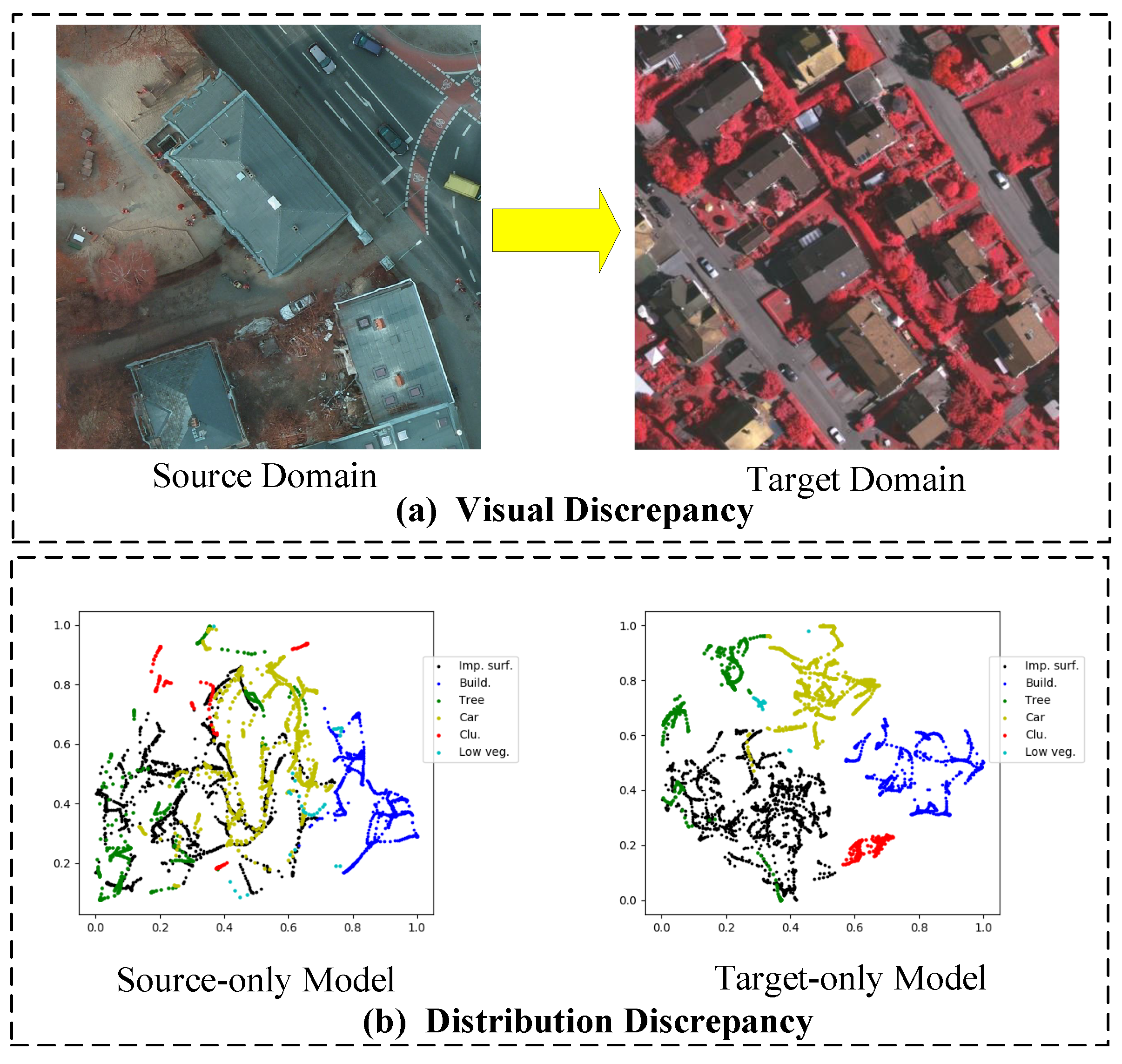
Figure 1. Two discrepancies in unsupervised cross-scene aerial image segmentation. (a) Visual discrepancy. The images in the source domain and target domain have different appearances (e.g., object textures, style representation) due to different locations, different sensors, different lighting, and so on. (b) Distribution discrepancy. Here, we map the high-dimensional features of the target image in the source-only model (without DA) and target-only model (full-supervision) into the 2D space with t-SNE [12] to reflect the inconsistent data distribution of the source domain and target domain. Each color in the distribution map represents a category.
Remotesensing 15 01207 g001
Figure 2. Samples of the over-adapted images and noisy pseudo labels in UDA semantic segmentation. (a) Over-adapted images. From left column to right: we provide the source image, target image, generated translated image utilizing CycleGAN [13], and ours. (b) Noisy pseudo labels. From the left column to the right: we present the image, the corresponding ground-truth, pseudo labels utilizing AdaptSegNet [20], and the corresponding error map. (Best viewed in color).
Remotesensing 15 01207 g002
Figure 3. Bidirectional learning vs. sequential learning.
Remotesensing 15 01207 g003
Figure 4. Structure of the proposed SLNet method for UDA semantic segmentation. The upper left part represents the spectral-based image translation model, responsible for the style transfer and identity preservation of source domain images. The lower left part denotes the segmentation adaptation model with pseudo-label revising, enabling a dynamic threshold to revise the noisy pseudo labels. The upper right part shows two discriminators at different levels. The lower right part shows the legend notes of this framework in detail.
Remotesensing 15 01207 g004
Figure 5. Visualization of decomposing images into low-frequency and high-frequency components with FFT [57].
Remotesensing 15 01207 g005
Figure 6. Diagram of self-supervised learning process in UDA semantic segmentation. (a) The upper-left part is a segmentation adaptation model and (b) the upper-right part represents the classical pseudo-label learning based on a manual threshold. (c) The lower-right part is our pseudo-label revising based on entropy minimization, while (d) the lower-left part denotes the legend notes.
Remotesensing 15 01207 g006
Figure 7. Experimental datasets. The upper, respectively, represents Vaihingen and Potsdam datasets for multi-category UDA semantic segmentation, showing the images and their corresponding ground truth labels, respectively. The lower indicates the Mass and Inria datasets for single-category UDA semantic segmentation.
Remotesensing 15 01207 g007
Figure 8. Qualitative results for single-category UDA semantic segmentation based on the Mass and Inria dataset. The first two lines are from Mass to Inria, and the last two lines are from Inria to Mass. Legend—white building surfaces, black background. The input images are cropped to 452 × 452 for better visualization.
Remotesensing 15 01207 g008
Figure 9. Qualitative results for multi-category UDA semantic segmentation on 6-class semantic segmentation from the Vaihingen to Potsdam dataset.
Remotesensing 15 01207 g009
Figure 10. Qualitative results for multi-category UDA semantic segmentation on the 6-class semantic segmentation from the Potsdam to Vaihingen dataset.
Remotesensing 15 01207 g010
Figure 11. Radar charts of mIoU (%) on 5-class UDA semantic segmentation from the Vaihingen to Potsdam dataset. On the left is the comparison between method A 2 and A 2 ( T ) , while the right is the comparison between method A 2 ( T ) and [ A 2 ] 1 ( T ) . Zoom in for details.
Remotesensing 15 01207 g011
Figure 12. Visual comparison between CycleGAN [13] and our spectral-based image translation model. Here, we show the visualization results of image translation from Vaihingen to Potsdam, Potsdam to Vaihingen, Mass to Inria, and Inria to Mass, respectively. The input images are cropped to 452 × 452 for better visualization.
Remotesensing 15 01207 g012
Figure 13. Visualization of the discrepancy between the error map, confidence map, and entropy map. Best viewed in color.
Remotesensing 15 01207 g013
Table 1. The quantitative results of our SLNet and the other state-of-the-art for single-category UDA semantic segmentation based on the Mass and Inria dataset. Here, the mIoU gap indicates the gap between the current model and target-only model. The bold represents the best performance. * means that this method is reproduced by ourselves.
Single-CategoryMass ⇒ InriaInria ⇒ Mass
ModelmIoUmIoU GapmIoUmIoU Gap
Source-only30.7952.7024.5254.04
ADDA * [64]43.5239.9733.3845.18
CyCADA * [46]45.8137.6939.8638.70
AdaptSegNet * [20]46.2837.2143.1735.39
ScaleNet * [37]50.2233.2746.4432.12
SRDA-Net [36]52.8630.64--
BDL * [25]54.1629.3348.6029.96
SLNet57.3226.1751.1627.40
Target-only83.490.0078.560.00
Table 2. The quantitative results of our SLNet and the other state-of-the-art for multi-category UDA semantic segmentation from the Vaihingen to Potsdam dataset. The bold entities represent the best performance. * means that this method is reproduced by ourselves.
Multi-CategoryVaihingen ⇒ Potsdam
ModelImp. Surf.Build.Low Veg.TreeCarmIoU(%)Mean F 1 (%)mIoU Gap(%)
Source-only19.0932.9822.595.538.0117.6420.9155.05
GAN-RSDA [34]18.6627.4019.7232.060.5919.6921.9653.00
SEANet [17]28.9036.248.705.1744.7724.7637.0447.93
AdaptSegNet * [20]43.1844.2639.8621.4111.2631.9944.9440.70
CyCADA * [46]45.3633.6229.1337.0716.4932.3346.5840.36
ADDA * [64]46.2942.2142.5426.2923.5636.1849.0536.51
BSANet [38]50.2149.9828.6727.6641.5139.6153.1933.08
Dual_GAN [65]45.9659.0141.7325.8039.7142.4458.7730.25
ScaleNet [37]49.7646.8252.9340.2342.9746.54-26.15
SRDA-Net [36]60.2061.0051.8036.8063.4054.64-18.05
CCDA_LGFA [66]64.3966.4447.1737.5559.3554.9870.2817.71
BDL * [25]61.5659.9844.0645.7066.0555.4772.0417.22
SLNet65.0565.8652.6354.0875.2562.5875.8510.11
Target-only77.1379.4560.0866.5680.2472.6983.740.00
Table 3. The quantitative results of our SLNet and the other state-of-the-art for multi-category UDA semantic segmentation from the Potsdam to Vaihingen dataset. The bold entities represent the best performance. * means that this method is reproduced by ourselves.
Multi-CategoryPotsdam ⇒ Vaihingen
ModelImp. Surf.Build.Low Veg.TreeCarmIoU(%)Mean F 1 (%)mIoU Gap(%)
Source-only40.3932.8124.1623.585.3325.2537.0253.09
GAN-RSDA [34]34.5540.6422.5824.949.9026.5240.7751.82
ADDA * [64]43.2852.1624.3928.8415.2632.7945.6845.55
SEANet [17]41.8456.8020.8321.8631.7234.6149.9843.73
CyCADA * [46]48.5960.0427.7136.8413.4937.3353.3741.01
AdaptSegNet * [20]51.9656.1925.6845.9730.1641.9958.4936.35
BSANet [38]53.5559.8723.9151.9327.2443.3062.6835.04
Dual_GAN [65]46.1965.4427.8555.8240.3147.1263.0131.22
ScaleNet [37]55.2264.4631.3450.4039.8647.66-30.68
BDL * [25]60.0567.4846.4265.4037.8156.6771.5221.67
CCDA_LGFA [66]67.7476.7547.0255.0344.9058.2970.0620.05
SLNet70.6276.7252.2268.3545.6262.7176.4215.63
Target-only79.3685.61572.9475.3278.4878.3487.610.00
Table 4. Ablation study of the sequential learning from Vaihingen to Potsdam. See the text for the specific description of notations. ’SSL’ denotes the method of self-supervised learning. ‘ K ’ represents the number of iterations. The bold represents the best performance.
MethodSSLKmIoU(%)
A 0 N-17.64
A 1 N-44.87
A 2 N-46.18
A 0 ( C ) N-41.76
A 1 ( C ) N-48.16
A 2 ( C ) N-50.81
A 0 ( T ) N-45.64
A 1 ( T ) N-50.29
A 2 ( T ) N-52.17
[ A 2 ] 1 ( T ) Y158.63
[ A 2 ] 2 ( T ) Y262.58
[ A 2 ] 3 ( T ) Y360.24
Table 5. The effect of the selection of super-parameters γ on the experimental performance of the model A 2 ( T ) and [ A 2 ] 1 ( T ) . Here, Δ ↑ indicates the mIoU gain. The bold represents the best performance.
Method γ mIoU (%) Δ
A 2 -46.180.00
A 2 ( T ) 0.0048.192.01
0.0150.344.16
0.0551.675.49
0.1051.915.73
0.1552.175.99
[ A 2 ] 1 ( T ) 0.0053.957.77
0.0155.889.70
0.0557.9211.74
0.1058.6312.45
0.1557.2711.09
Table 6. Performance comparison between manual threshold and entropy minimization from Vaihingen to Potsdam. Here, ‘+ Pseudo-label Learning’ denotes that the model is trained on the basis of A 2 ( T ) by utilizing the pseudo-label with confidence. Our [ A 2 ] 1 ( T ) does not set the manual threshold. The bold represents the best performance.
MethodThresholdmIoU (%)
A 2 ( T ) -52.17
+ Pseudo-label Learning0.9553.71
0.9055.88
0.8556.42
0.8055.17
0.7555.49
0.7054.38
[ A 2 ] 1 ( T ) -58.63
Table 7. The influence of the selection of metric functions on the adaptive performance of the methods. The bold entities represent the best performance.
MethodMetric FunctionsmIoU (%)
[ A 2 ] 1 ( T ) MMD [67]55.25
KL-divergence56.94
JS-divergence58.63
Disclaimer/Publisher’s Note: The statements, opinions and data contained in all publications are solely those of the individual author(s) and contributor(s) and not of MDPI and/or the editor(s). MDPI and/or the editor(s) disclaim responsibility for any injury to people or property resulting from any ideas, methods, instructions or products referred to in the content.