Reducing the Influence of Systematic Errors in Interference Core of Stepped Micro-Mirror Imaging Fourier Transform Spectrometer: A Novel Calibration Method

Abstract

The stepped micro-mirror imaging Fourier transform spectrometer (SIFTS) has the advantages of high throughput, compactness, and stability. However, the systematic errors in the interference core of the SIFTS have a significant impact on the interferogram and the reconstructed spectrum. In order to reduce the influence of systematic errors, a transfer error model of the systematic errors in the interference core of the SIFTS is established, and an interferogram and spectrum calibration method is presented, which combines the least squares fitting calibration and the row-by-row fast Fourier transform-inverse fast Fourier transform (FFT-IFFT) flat-field calibration. The experimental results show that the methods can sufficiently reduce the influence of systematic errors in the interference core of the SIFTS, such as the interferogram fringe tilt, the peak position shift of the reconstructed spectrum, and the error of spectral response.

1. Introduction

Imaging Fourier transform spectroscopy (IFTS) can simultaneously acquire two-dimensional spatial information and one-dimensional spectral information [1,2,3], and has a high spectral resolution, high throughput, high stability, strong targeting, high sensitivity, strong adaptability, long service life, and other advantages [4,5,6], so it is widely used in environmental monitoring and atmospheric remote sensing and other fields [7,8,9,10,11,12,13]. Based on the structure of the Michelson interferometer, we proposed a stepped micro-mirror imaging Fourier transform spectrometer (SIFTS), which greatly improves stability and ensures high throughput and a certain spectral resolution [14,15,16].

As an interferometric hyperspectral analysis instrument, the SIFTS has extremely high requirements for the assembly and adjustment accuracy of each component, especially the interference core composed of the plane mirror, the stepped micro-mirror, the beam splitter, and the compensation plate. The micron-level optical misalignment in the interference core will cause large systematic errors in the interferogram and the reconstructed spectrum. Since the installation accuracy of the beam splitter and the compensation plate is highly related to the processing accuracy of the interference core frame, the optical misalignment can be controlled within a negligible range. However, due to the large adjustable dimensions and difficulty of the assembly and adjustment of the stepped micro-mirror and plane mirrors, there will be some inevitable small optical misalignments, which require large, high-precision optical mounts and very careful alignment to calibrate. These calibration measures greatly increase the difficulty of assembly and adjustment, and affect the compactness and stability of the SIFTS. Therefore, a calibration method in the post-processing stage is needed to reduce the influence of these systematic errors.

There have been some research reports on the systematic error correction of interferometric spectrometers. Xiang et al. systematically analyzed the influence of the moving mirror tilt in the Fourier transform spectrometer on the degree of interference modulation and phase [17]. Gao et al. analyzed the influence of the rotating mirror tilt in the rotating mirror interference spectrometer on the degree of interference modulation and phase [18]. Zeng et al. analyzed the influence of different tilt directions of the moving mirror in the Fourier transform spectrometer on the system error [19]. Liu et al. analyzed the influence of the error of the tilt mirror in the spatial modulation Fourier transform spectrometer on the phase, spectral resolution, and signal-to-noise ratio [20]. Feng et al. analyzed the influence of the tilt error of the moving mirror on the circular aperture in the Fourier transform spectrometer, and proposed a dynamic calibration method [21]. Barnett et al. proposed a method to calibrate the interference fringe error [22]. Jin et al. analyzed the effect of detector alignment error on spectral resolution and gave error tolerance limits [23]. Zou et al. proposed a spectral fitting calibration method based on spectral refinement [24]. Feng et al. analyzed the reference atmospheric radiation transmission pattern and proposed a Fourier transform spectrometer on-orbit spectral calibration method [25]. Cui et al. proposed a radiation calibration method for micro spectrometer based on the Lagrangian interpolation algorithm [26]. Lv et al. proposed a radiation calibration method based on reflectivity parameters, simulation data and in-orbit measurement data comparison [27].

It can be seen that the current related research has mainly analyzed the influence of the systematic error in the interference system on the spectral phase and has seldom analyzed the influence of the systematic error on the spectral wavenumber. As well, the current research related to interferogram and spectral calibration methods is mainly for the improvement of traditional calibration methods in applications, and lacks integration with the analysis of systematic error modulation and transmission mechanisms of instruments. The special structure of the SIFTS interference core (the stepped micro-mirror) makes the systematic error have a significant impact on the spectral wavenumber and the interferogram. Therefore, in order to improve the measurement accuracy and reduce the difficulty of installation and adjustment, the relationship between the systematic error in the interference core of SIFTS and the spectral wavenumber error and the interferogram is analyzed in this paper. First, by analyzing the optical misalignment of the interference core, a transfer error model of the systematic error is established. Then, according to the transfer error model, an interferogram and spectrum calibration method combining least squares fitting correction and row-by-row fast Fourier transform-inverse fast Fourier transform (FFT-IFFT) flat-field correction is presented, which can reduce the influence of the systematic error in the interference system on the interferogram and the reconstructed spectrum, and reduce the difficulty of assembly and adjustment. Finally, in order to verify the method, we built an experimental verification platform and conducted verification experiments. The experimental results show that the method has a relatively good correction effect on various problems caused by the systematic error in the interference core of the SIFTS, such as the interferogram fringe tilt, the peak position shift of the reconstructed spectrum, and the spectral response error.

2. The Structure and Working Principle of SIFTS

Figure 1a shows the simplified configuration and mechanism for obtaining information about the SIFTS. Figure 1b shows the internal structure of the principle prototype, including a scanning mirror, a first imaging system, a plane mirror, a beam splitter, a compensation plate, a stepped micro-mirror, a second imaging system, and a detector with a cold stop.

The working principle of the SIFTS is that at a certain time, the light emitted by the target object passes through the scanning mirror and first imaging system, forming two primary image points on the plane mirror and the stepped micro-mirror, respectively. The two primary image points are ultimately imaged through the second imaging system on the focal plane of the detector, after being reflected by the plane mirror and micro-mirror. The difference in height between the plane mirror and micro-mirror causes the optical path differences (OPDs) between the two beams reaching the detector, thereby forming interference fringes on the detector. Therefore, image and spectral information regarding the target reaches the detector. Then the scanning mirror rotates, and the target is imaged on the next step surface, so the detector can obtain interference information concerning the different OPDs of the target. The interference intensity distribution can be expressed in the following form:

$$I(\delta )={\displaystyle \underset{-\infty }{\overset{+\infty }{\int }}B(\nu )}\exp (i2\pi \nu \delta )d\nu$$

(1)

where ν is the wave number of the incident light, δ is the OPD of the SIFTS system, and B(ν) is the power spectral density of the incident light. The input spectrum can be obtained by Fourier transform:

$$B(\nu )={\displaystyle \underset{-\infty }{\overset{+\infty }{\int }}I(\delta )}\exp (-i2\pi \nu \delta )d\delta$$

(2)

After one scan period, the detector obtains a three-dimensional data cube containing two-dimensional spatial information and one-dimensional spectral information. The IR images and spectra of the target are obtained by demodulating and processing the interference data for the data cubes according to the scanning order and OPD order.

The interference core of the SIFTS uses a stepped micro-mirror, which has 128 substeps with a height of 0.625 μm and a width of 0.25 mm, thereby obtaining a theoretical spectral resolution of 62.5 cm⁻¹. The SIFTS uses a mid-wave infrared HgCdTe area array detector with a response spectrum of 3.7~4.8 μm, the number of pixels is 320 × 256, and the pixel size is 30 μm × 30 μm.

3. Transfer Error Model of the Interference Core

The establishment of the transfer error model of the interference core requires a clear definition of the source of the error and its functional relationship with the interferogram or the reconstructed spectrum. Figure 2 shows the corresponding relationship between the two dimensions of the interferogram and the two dimensions of the stepped micro-mirror and the plane mirror, as well as the main source of the interference core systematic error (the black part in Figure 2b represents the stepped micro-mirror, and the red part represents the virtual image of the plane mirror).

As shown in Figure 2a, the interferogram of the SIFTS can be divided into two dimensions. The lateral interference dimension is modulated by the OPD sequence, which corresponds to the height change direction of the stepped micro-mirror in Figure 2b. The longitudinal spatial dimension corresponds to the longitudinal coordinates of the stepped micro-mirror and the virtual image of the plane mirror in Figure 2b. As shown in Figure 2b, the systematic errors of the interference core all come from the misalignment of the stepped micro-mirror and the plane mirror in different dimensions. Since the error introduced by the misalignment of the stepped micro-mirror and the plane mirror in the same dimension are similar, the errors of the two elements can be combined and analyzed. Therefore, the systematic error of the interference core can be divided into three categories: tilt error, slope error, and rotation error.

3.1. Tilt Error

Suppose the ideal spatial sampling interval (twice the height of the stepped micro-mirror) is δ₀, and the spatial interference dimension coordinate is x, then OPD can be expressed as a function of x: δ = δ₀∙x. Figure 3 shows the simplified model of the tilt error analysis of a stepped micro-mirror or a plane mirror. Suppose the tilt angle is α, the distance between the reflecting surface and the detector array is L, and the interference dimension coordinate of the tilt axis center is x₀.

When the stepped micro-mirror or flat mirror has a tilt error, its reflecting surface deviates from the standard position of the interference dimension, and the incident light will also deviate from the optical axis direction after being reflected by the reflecting surface, thus introducing an OPD error ε_x at each sampling position of the spatial interference dimension. According to the geometric relationship in Figure 3, ε_x can be expressed as a function of the interference dimension coordinate x:

$${\epsilon }_x=x\tan \alpha (\frac{\cos 2\alpha +1}{\cos 2\alpha })+[(\frac{2\cos 2\alpha -1}{\cos 2\alpha })L-x_0\tan \alpha (\frac{\cos 2\alpha +1}{\cos 2\alpha })]$$

(3)

Then the OPD after introducing the tilt error is:

$${\delta }^{\prime }=\delta +{\epsilon }_x=\frac{{\delta }_0+\tan \alpha (\frac{\cos 2\alpha +1}{\cos 2\alpha })}{{\delta }_0}\cdot \delta +\frac{(2\cos 2\alpha -1)L-x_0\tan \alpha (\cos 2\alpha +1)}{\cos 2\alpha }$$

(4)

In addition, we can see in Figure 3 that the existence of the tilt angle will make the structure of the stair-step micro-mirror resemble a blazed grating, causing the incident light to be diffracted onto the stepped micro-mirror, so that the fundamental frequency of the interference fringe spatial frequency changes from 0 to the Littrow wave number (the Littrow wave number is determined by the Littrow angle, that is, the tilt angle α of the stepped micro-mirror) [28,29,30]. Then, the interference intensity distribution becomes:

$$I^{\prime }(\delta )={\displaystyle \underset{-\infty }{\overset{+\infty }{\int }}B(\nu )}\exp [i2\pi 2(\nu -{\nu }_{Littrow})\tan \alpha {\delta }^{\prime }]d\nu$$

(5)

Substituting Equation (4) into Equation (5), we can obtain:

$$\begin{array}{cc}\hfill I^{\prime }(\delta )=& {\displaystyle \underset{-\infty }{\overset{+\infty }{\int }}B(\nu )}\exp (i2\pi 2(\nu -{\nu }_{Littrow})\tan \alpha [\frac{{\delta }_0+\tan \alpha (\frac{\cos 2\alpha +1}{\cos 2\alpha })}{{\delta }_0}\cdot \delta +\hfill \\ & \frac{(2\cos 2\alpha -1)L-x_0\tan \alpha (\cos 2\alpha +1)}{\cos 2\alpha })]d\nu \hfill \end{array}$$

(6)

Equation (6) can be further organized to obtain:

$$\begin{array}{cc}\hfill B^{\prime }(\nu )=& B\{\frac{\nu -2{\nu }_{Littrow}\tan \alpha [1+\frac{1}{{\delta }_0}\tan \alpha (\frac{\cos 2\alpha +1}{\cos 2\alpha })]}{1-2\tan \alpha [1+\frac{1}{{\delta }_0}\tan \alpha (\frac{\cos 2\alpha +1}{\cos 2\alpha })]}\}\times \hfill \\ & \exp \{i2\pi 2\frac{(\nu -{\nu }_{Littrow})\frac{(2\cos 2\alpha -1)L-x_0\tan \alpha (\cos 2\alpha +1)}{\cos 2\alpha }}{1-2\tan \alpha [1+\frac{1}{{\delta }_0}\tan \alpha (\frac{\cos 2\alpha +1}{\cos 2\alpha })]}\tan \alpha \}\hfill \end{array}$$

(7)

It can be seen that the tilt error changes the frequency domain sampling interval and introduces a fixed wavenumber drift and a certain phase error. The phase error will not affect the mode of the spectrum, so it can be ignored in the process of spectrum calibration. However, the change in the frequency domain sampling interval and the fixed wavenumber drift will have a greater impact on the accuracy of the peak position of the spectrum, and calibration is required. According to Equation (7), the wavenumber change after introducing the tilt error can be obtained:

$${\nu }_{Tilt}=\frac{\nu }{1-2\tan \alpha [1+\frac{1}{{\delta }_0}\tan \alpha (\frac{\cos 2\alpha +1}{\cos 2\alpha })]}-\frac{2{\nu }_{Littrow}\tan \alpha [1+\frac{1}{{\delta }_0}\tan \alpha (\frac{\cos 2\alpha +1}{\cos 2\alpha })]}{1-2\tan \alpha [1+\frac{1}{{\delta }_0}\tan \alpha (\frac{\cos 2\alpha +1}{\cos 2\alpha })]}$$

(8)

Except for ν_Tilt and ν, all the others in Equation (8) are constants. In order to simplify the subsequent calculation, Equation (8) can be written as follows:

$${\nu }_{Tilt}=k_{Tilt}\nu +b_{Tilt}$$

(9)

where k_Tilt and b_Tilt are the transfer error coefficients, and the specific values are:

$$\{\begin{array}{l}{k}_{Tilt}=\frac{1}{1-2\tan \alpha [1+\frac{1}{{\delta }_0}\tan \alpha (\frac{\cos 2\alpha +1}{\cos 2\alpha })]}\\ b_{Tilt}=-\frac{2{\nu }_{Littrow}\tan \alpha [1+\frac{1}{{\delta }_0}\tan \alpha (\frac{\cos 2\alpha +1}{\cos 2\alpha })]}{1-2\tan \alpha [1+\frac{1}{{\delta }_0}\tan \alpha (\frac{\cos 2\alpha +1}{\cos 2\alpha })]}\end{array}$$

(10)

3.2. Slope Error

Figure 4 shows the simplified slope error analysis model of a stepped micro-mirror or a plane mirror. Suppose the slope angle is β, the distance between the reflecting surface and the detector array is L, and the spatial dimension coordinate of the slope axis is y₀.

When we only consider the slope error of the stepped micromirror or plane mirror, the reflecting surface will also deviate from the standard position of the interference dimension, so that the incident light will deviate from the optical axis direction after being reflected by the reflecting surface, but the offset only changes with the spatial dimension coordinates. According to the geometric relationship in Figure 4, the slope error can be expressed as:

$${\epsilon }_y=y\tan \beta (1+\frac{1}{\cos 2\beta })-(L-y_0\tan \beta )(1+\frac{1}{\cos 2\beta })+2L$$

(11)

The spatial sampling interval has also changed:

$${{\delta }_0}^{\prime }={\delta }_0\frac{1+\cos 2\beta }{\cos \beta }$$

(12)

Substituting ε_y and δ₀′ into Equation (1), we can obtain:

$$\begin{array}{cc}\hfill I^{\prime }(\delta )=& {\displaystyle \underset{-\infty }{\overset{+\infty }{\int }}B(\nu )}\exp \{i2\pi \nu [{\delta }_0\frac{1+\cos 2\beta }{\cos \beta }+\hfill \\ & y\tan \beta (1+\frac{1}{\cos 2\beta })-(L-y_0\tan \beta )(1+\frac{1}{\cos 2\beta })+2L]\}d\nu \hfill \end{array}$$

(13)

Equation (13) can be further organized to obtain:

$$\begin{array}{cc}\hfill B^{\prime }(\nu )=& B(\nu \frac{\cos \beta }{1+\cos 2\beta })\exp [i2\pi \nu \frac{\cos \beta }{1+\cos 2\beta }+\hfill \\ & y\tan \beta (1+\frac{1}{\cos 2\beta })-(L-y_0\tan \beta )(1+\frac{1}{\cos 2\beta })+2L]\hfill \end{array}$$

(14)

It can be seen that the slope error changes the frequency domain sampling interval and introduces a certain phase error. Similar to the case of the tilt error, ignoring the phase error, the wavenumber relationship before and after the slope error can be obtained:

$${\nu }_{Slope}=\frac{\cos \beta }{1+\cos 2\beta }\nu$$

(15)

Except for ν_Slope and ν, all the other variables in Equation (15) are constants. In order to simplify the subsequent calculation, Equation (15) can be written as follows:

$${\nu }_{Slope}=k_{Slope}\nu$$

(16)

where k_Slope is the transfer error coefficients, and the specific values is:

$$k_{Slope}=\frac{\cos \beta }{1+\cos 2\beta }$$

(17)

3.3. Rotation Error

Figure 5 shows the simplified rotation error analysis model of a stepped micro-mirror or a plane mirror. Suppose the rotation angle is γ, and the rotation center coordinate is (x_γ, y_γ).

It can be seen that the rotation error will not introduce the OPD error but will cause the overall translation of the interference sequence of each row, that is, the rotation of the interference fringes. The translation of the interference sequence can be expressed as:

$$\mathsf{\Delta }x=x-x_{\gamma }=(y-y_{\gamma })\tan \gamma$$

(18)

According to the Fourier transform displacement theorem [31], the effect of the interference sequence translation on the spectrum can be expressed as:

$$B^{\prime }(\nu )=ℱ\{I[(x-(y-y_{\gamma })\tan \gamma ){\delta }_0])\}=B(\nu )\exp [-i2\pi {\delta }_{0}x(y-y_{\gamma })\tan \gamma ]$$

(19)

Equation (17) shows that the rotation error will not bring about a frequency shift, but only a phase shift, so it can be ignored in the spectral calibration. However, in the radiation calibration, it is necessary to calibrate the relative radiation response of the pixels of the same interference order, and the rotation of the fringes will cause the pixels in the same column in the longitudinal direction to no longer be in the same interference order, so the difficulty of calibrating the relative radiation response between the pixels of the same interference order is greatly increased.

3.4. Transfer Error Model

The analysis in Section 3.1, Section 3.2 and Section 3.3 shows that the major influences on the spectrum are the tilt error and the slope error, and the wavenumber shift caused by these two errors is linear, which can be organized into a transfer error model:

$${\nu }^{\prime }=k\nu +b$$

(20)

where k and b are the transfer error coefficients, and the specific values are:

$$\{\begin{array}{l}k=k_{Tilt}+k_{Slope}=\frac{1}{1-2\tan \alpha [1+\frac{1}{{\delta }_0}\tan \alpha (\frac{\cos 2\alpha +1}{\cos 2\alpha })]}+\frac{\cos \beta }{1+\cos 2\beta }\\ b=b_{Tilt}=-\frac{2{\nu }_{Littrow}\tan \alpha [1+\frac{1}{{\delta }_0}\tan \alpha (\frac{\cos 2\alpha +1}{\cos 2\alpha })]}{1-2\tan \alpha [1+\frac{1}{{\delta }_0}\tan \alpha (\frac{\cos 2\alpha +1}{\cos 2\alpha })]}\end{array}$$

(21)

It can be seen that the transfer error model is a linear form. Due to the high integration of the SIFTS interference core, some precision measurement tools are difficult to apply and the parameters in Equation (21) are very difficult to measure. Therefore, in the calibration process, it is only necessary to measure the peak wavenumbers of at least two standard narrowband radiation sources with different central wavenumbers, and substitute them into Equation (20) together with the theoretical central wavenumbers to obtain the transfer error coefficients k and b, and then complete for wavenumber calibration, there is no need to calculate the parameters in Equation (21).

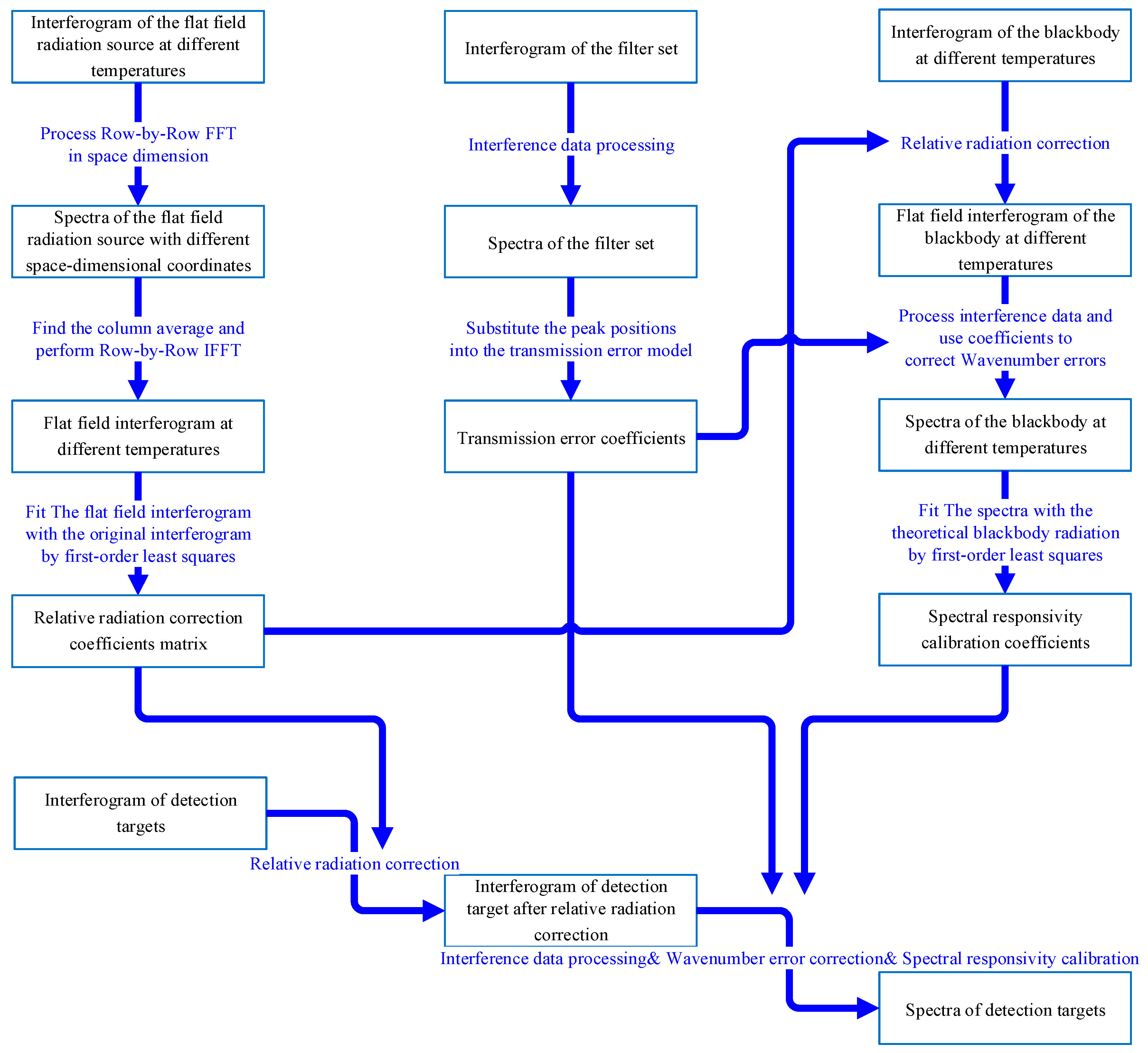
4. Calibration Method and Experimental Design

4.1. Calibration Method

The calibration process of the static Fourier transform spectrometer is as follows [32,33]. First, the relative radiation response between the pixels of the same interference order of the interferogram is calibrated in the spatial domain. Then, spectral calibration is performed, and finally, spectral responsivity is calibrated in the frequency domain. It can be seen in Section 3 that the systematic errors of the interference core mainly cause the fringe rotation of the interferogram and the wavenumber shift of the spectrum. The rotation of the interference fringes will cause the pixels in the same column in the longitudinal direction to no longer be in the same interference order, so the difficulty of calibrating the relative radiation response between the pixels of the same interference order is greatly increased. The wavenumber shift of the spectrum will increase the difficulty of spectral calibration, which in turn affects the spectral responsivity calibration in the frequency domain.

Aiming at the influence of the systematic error of the interference core, we propose a new calibration method, based on the transfer error model in Section 3 and combined with the least squares method and progressive FFT-IFFT to calibrate the interference data. The calibration flow chart is shown in Figure 6:

The calibration process can be mainly divided into three parts. The first part is the calibration of the relative radiation response of the pixels of the same interference order, the second part is the calibration of the spectral wavenumber, and the third part is the calibration of the spectral responsivity.

The first part is the calibration of the relative radiation response of the pixels of the same interference order. Aiming at the rotation of the interference fringes caused by the rotation error, we propose a row-by-row FFT-IFFT relative radiation response calibration method. First, measure the interferograms of flat-field radiation sources with different temperatures. Due to the possible rotation error of the interference core, the interference fringes will have a certain rotation, which causes the pixels of the same interference order to no longer be in the same column, which cannot be solved by averaging the columns. According to the analysis in Section 3.3, the rotation error will cause the overall translation of the interference sequence of each row, thereby introducing a phase shift in the frequency domain without introducing a wavenumber shift. Therefore, the interferogram can be subjected to row-by-row fast Fourier transform, and the column average can be obtained after transforming to the frequency domain, and then the inverse Fourier transform IFFT can be performed to obtain the interferogram corresponding to the calibration of the relative radiation, as shown in Figure 7. Finally, the interferograms of the corrected flat-field radiation sources with different temperatures and the original interferograms are fitted by the pixel-by-pixel first-order least squares method to obtain the relative radiation response calibration coefficient matrix.

In the second part of the spectral wavenumber calibration, according to the analysis in Section 3.1 and Section 3.2, the systematic error of the interference core will cause the spectral wavenumber to drift linearly. According to the specific form of the transfer error model, a group of standard narrowband radiation sources with different central wavenumbers is selected, their interferograms are obtained, and the relative radiation response calibration coefficient matrix obtained in the first part is used for calibration. Then the interference data are processed to obtain the measured central wavenumber, and finally, first-order least squares fitting is performed with the theoretical central wavenumber to obtain the spectral transfer error coefficients k and b.

The third part is the spectral responsivity calibration. In this part, a temperature range and sampling interval are set, the instrument is used to obtain the interferogram of the blackbody corresponding to the temperature, and the relative radiation response calibration coefficient matrix obtained in the first part is used for calibration. Then the interference data are processed to obtain the blackbody spectrum, and the spectral error transfer coefficients k and b obtained in the second part are used to perform spectral calibration. Finally, the first-order least squares fitting is performed between the measured blackbody spectrum and the theoretical blackbody spectrum corresponding to the temperature, and the spectral response calibration coefficient can be obtained.

After all three calibration coefficients are obtained, the spectral data of any detection target can be calibrated.

4.2. Experimental Design

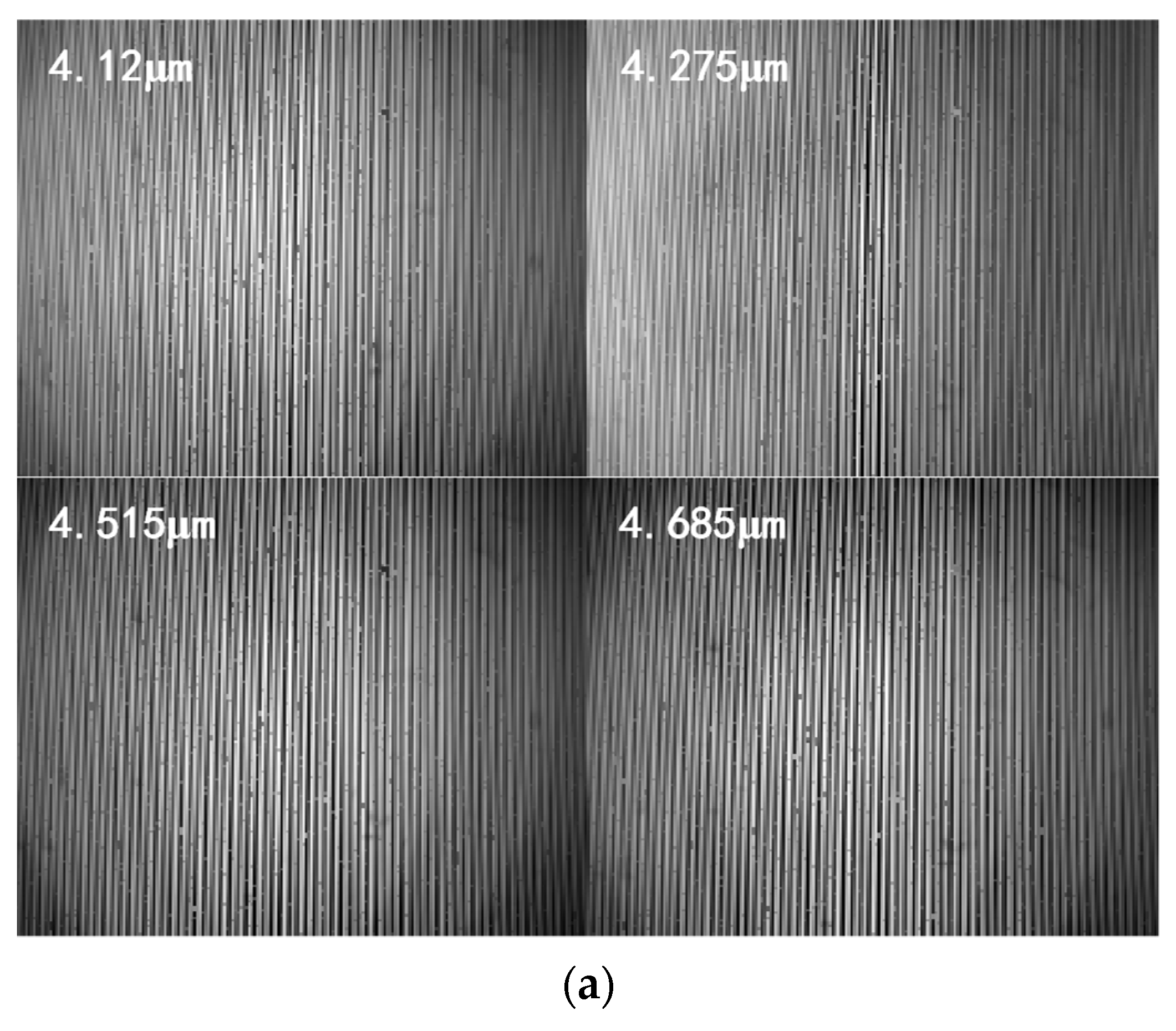
According to the calibration method in Section 4.1, during the calibration experiment, we needed to measure mainly flat-field radiation sources with different temperatures, standard narrow-band radiation sources with different central wavenumbers, and standard blackbodies with different temperatures. Figure 8 shows the schematic and photograph of the laboratory calibration system of the SIFTS. The flat-field radiation source consisted of a calibrated standard point source blackbody and a beam expander system. The end of the beam expander system can add and replace narrow-band filters, which can simulate standard narrow-band radiation sources with different center wavelengths.

Figure 9 shows the image plane intensity distribution of the effective area of the point light source imaged by the beam expander system simulated by the simulation software. After calculation, the flatness of the effective imaging area of the image plane was 99.98%, which can basically be regarded as a flat-field radiation source.

After the calibration was complete, further verification of the calibration results was required. Considering the response band of the SIFTS, we used a liquid sample glass slide made of acetonitrile with a strong absorption peak around 2273 cm⁻¹ to verify the effect of spectral wavenumber calibration, and the standard blackbody spectrum of the temperature point not used in the calibration was used to verify the effects of relative radiation response calibration and the spectral response calibration.

5. Experimental Results and Discussion

5.1. Relative Radiation Response Calibration

We set 10 temperature points in the temperature range of 338 K–373 K (the temperature range is a common range for SIFTS in applications), measured the flat-field radiation source corresponding to the temperature, selected the effective interference area, and obtained the interferograms as shown in Figure 10:

We took the interferogram of a 338 K radiation source as an example of the specific calibration process. In order to clearly show the characteristics of the interference data, the subsequent processing is displayed in pseudo-color. Figure 11 shows the two-dimensional interferogram of the 338 K radiation source and its three-dimensional curved surface.

It can be seen that the interference fringes had obvious rotation, the baseline is greatly distorted, and the response uniformity of the pixels of the same interference order is poor. The relative radiation response calibration was performed using the row-by-row FFT-IFFT method proposed in Section 4.1. Since there were two pixels on an interference order in the interferometric dimension, the interferogram was split into two parts and processed separately. The frequency domain distribution obtained by row-by-row FFT, the frequency domain distribution after column averaging, and the corrected interferogram obtained after row-by-row IFFT are shown in Figure 12.

Figure 12a,b shows the spatial distribution of the one-dimensional spectrum obtained after baseline correction and the row-by-row FFT of the interference data of the flat-field radiation source on two pixels in the same order (the left-right symmetry is due to the conjugate symmetry effect of the Fourier transform). Since the rotation of the interference fringes had no effect on the peak position of the frequency domain spectrum, the column average could be directly obtained. Figure 12c,d shows the distribution of the one-dimensional spectrum in the spatial dimension after the column average. We performed row-by-row IFFT on Figure 12c,d and rearranged the same-level pixels to obtain Figure 12e,f, that is, the interferogram after relative radiation calibration. It can be seen that the rotation of the interference fringes and the poor uniformity of the response of the same interference order pixel were greatly improved. Then, the above-mentioned processing was performed on the interferogram of the flat-field radiation source corresponding to each temperature point, and finally, the calibration coefficient of the relative radiation response of each pixel was obtained by first-order least squares fitting, as shown in Figure 13:

5.2. Spectral Wavenumber Calibration

In this part, we selected a set of narrow-band filters with center wavelengths of 4.12 μm, 4.275 μm, 4.515 μm, and 4.685 μm (the half-peak widths are all smaller than the theoretical spectral resolution of the SIFTS), which were installed in the beam expander system. Then we measured their interferograms (blackbody temperature of 500 K). Finally, the interference data of the interferograms of the filter set were processed to obtain the spectra. The interferograms and spectra of the filter settings are shown in Figure 14:

Due to the low theoretical spectral resolution of the SIFTS, in order to reduce the influence of the fence effect, the zero-padding method was used to increase the wavenumber accuracy of the spectrum in the process of the interference data processing, and the zero-padding multiple was selected to be 100 times. The measured spectral center wavenumbers of the filter set were 2350.7 cm⁻¹, 2562.7 cm⁻¹, 2862.2 cm⁻¹, and 3055.6 cm⁻¹, which have large errors with the theoretical values of 2427.2 cm⁻¹, 2339.2 cm⁻¹, 2214.8 cm⁻¹, and 2134.5 cm⁻¹. The central wavenumber of the filter set was substituted into the transfer error model, that is, Equation (20), and k was obtained as −0.4152 and b as 3403.3. Then, the transfer error model was obtained as:

$${\nu }^{\prime }=-0.4152\nu +3403.3431$$

(22)

The transfer error model was used to calibrate the filter set spectra, and the filter set spectra were obtained after the spectral wavenumber calibration, as shown in Figure 15:

The central wavenumbers of the calibrated spectrum were 2427.3 cm⁻¹, 2339.3 cm⁻¹, 2214.9 cm⁻¹, and 2134.7 cm⁻¹, and the average error from the theoretical value was only 0.0056%. Moreover, it can be seen that the systematic error of the interference core not only introduced a large wavenumber error but also caused a serious broadening of the spectrum, which greatly reduced the resolution. The wavenumber calibration can simultaneously calibrate the wavenumber error and spectral broadening.

5.3. Spectral Response Calibration

In this section, we continue to use the data measured in the relative radiation response calibration, performing a relative radiation calibration of the interferogram using the relative radiation response calibration coefficient matrix obtained in Section 5.1, and then perform the interference data processing, using the transfer error model obtained in Section 5.2 to perform the wavenumber calibration to obtain the spectral responses of blackbodies at different temperatures. The spectral response calibration coefficient can be obtained by fitting the measured blackbody spectral response with the theoretical blackbody radiation by the first-order least squares method. The measured spectral response of the blackbody at different temperatures, the theoretical blackbody radiation, the spectral response calibration coefficient, and the calibrated blackbody spectral response are shown in Figure 16:

Figure 16 shows that the relative error between the blackbody spectrum after the spectral response calibration and the theoretical value was 1.32%.

5.4. Verification of Calibration Methods

In this section, we verify the calibration method. According to the experimental design in Section 4.2, we used a liquid sample glass slide made of acetonitrile with a strong absorption peak around 2273 cm⁻¹ to verify the effect of the spectral wavenumber calibration, and used the standard blackbody spectrum of 333 K to verify the effects of the relative radiation response calibration and the spectral response calibration. The results obtained are shown in Figure 17:

Figure 17a shows that the measured central wavenumber of the acetonitrile was 2273.8 cm⁻¹, and the error from the theoretical value of 2273 cm⁻¹ was only 0.035%. Figure 17b shows that the relative error between the blackbody spectrum after the spectral response calibration and the theoretical value was 4.49%, and the relative error was further reduced to 2.01% after the relative radiation response calibration. It can be seen that the errors of the spectral peak positions and spectral response are higher than the results in Section 5.2 and Section 5.3. This is due to the fact that the original data in Section 5.2 and Section 5.3 were the actual measured values used to fit the calibration equation, and the errors between their calibration values and the ideal values are mainly fitting error. In contrast, the original data in Section 5.4 were not used to fit the calibration equation, and the error between its calibration value and the ideal value is mainly the prediction error, which is generally higher than the fitting error. Therefore, the spectral wavenumber calibration method, the relative radiation response calibration method, and the spectral response calibration method are effective.

In addition, to explore the effectiveness of the method in practical application, we conducted an outfield experiment at a plant, and the detection area was the emission area of a gas boiler, as shown in Figure 18a. The experimentally acquired original data were processed to obtain the infrared image of the detection region and the transmittance spectrum of the target region as shown in Figure 18b.

The target area selected in Figure 18b (in the red box) is the emission from the gas boiler, which typically consists of water vapor, carbon dioxide, oxygen and nitrogen. Among them, only carbon dioxide has a relatively strong absorption peak in the range of 3.7–4.8 μm, specifically in the range of 4.16–4.54 μm (2200–2400 cm⁻¹), which is consistent with the results in Figure 18b. Thus, the effectiveness of the method was further validated.

6. Conclusions

For the SIFTS, the systematic error in the interference core has a significant impact on the interferogram and the reconstructed spectrum. In this paper, we divided the systematic error into three types—tilt error, slope error, and rotation error—and established the transfer error model, showing that the systematic error in the interference core will cause a linear shift of the spectral wavenumber, and may also cause an interference fringe rotation of the interferogram. Combined with the transfer error model and instrument principle, we proposed an interferogram and spectrum calibration method combining least square fitting correction and row-by-row FFT-IFFT flat-field correction and built an experimental platform to verify the method.

The experimental results show that the relative radiation response calibration can eliminate the rotation of interference fringes caused by rotation error, and reduce the relative error of the spectral response. Spectral wavenumber calibration can calibrate the wave number linear shift and spectral broadening caused by tilt error and slope error. Spectral response calibration can calibrate the non-uniform spectral response of the detector in the response band. In general, the method proposed in this paper can improve the detection accuracy of the SIFTS in the data processing stage, and reduce the difficulty of the assembly and adjustment of the interference core to a certain extent. Due to the structural similarity of the interference imaging spectrometer, this method has certain universality.

References

1. Griffiths, P.R.; Haseth, J.A. Fourier Transform Infrared Spectrometry, 2nd ed.; Wiley: Hoboken, NJ, USA, 1983; pp. 312–314. [Google Scholar]
2. Yang, C.; Zhou, Z.Y.; Li, Y.; Liu, S.K.; Ge, Z.; Guo, G.C.; Shi, B.S. Angular-spectrum-dependent interference. Light Sci. Appl. 2021, 10, 217. [Google Scholar] [CrossRef]
3. Israelsen, N.M.; Petersen, C.R.; Barh, A.; Jain, D.; Jensen, M.; Hannesschläger, G.; Tidemand-Lichtenberg, P.; Pedersen, C.; Podoleanu, A.; Bang, O. Real-time high-resolution mid-infrared optical coherence tomography. Light Sci. Appl. 2019, 8, 11. [Google Scholar] [CrossRef]
4. Saptari, V. Fourier Transform Spectroscopy Instrumentation Engineering, 1st ed.; SPIE Optical Engineering Press: Bellingham, WA, USA, 2003; pp. 4–8. [Google Scholar]
5. Talghader, J.J.; Gawarikar, A.S.; Shea, R.P. Spectral selectivity in infrared thermal detection. Light Sci. Appl. 2012, 1, e24. [Google Scholar] [CrossRef]
6. Li, A.; Yao, C.; Xia, J.; Wang, H.; Cheng, Q.; Penty, R.; Fainman, Y.; Pan, S. Advances in cost-effective integrated spectrometers. Light Sci. Appl. 2022, 11, 174. [Google Scholar] [CrossRef]
7. Zhang, C.; Zhao, B.; Bin, X.; Li, Y. Interference image spectroscopy for upper atmospheric wind field measurement. Optik 2006, 117, 265–270. [Google Scholar] [CrossRef]
8. Girshovitz, P.; Shaked, N.T. Doubling the field of view in off-axis low-coherence interferometric imaging. Light Sci. Appl. 2014, 3, e151. [Google Scholar] [CrossRef]
9. Pope, A.; Rees, W.G. Impact of spatial, spectral, and radiometric properties of multispectral imagers on glacier surface classification. Remote Sens. Environ. 2014, 141, 1–13. [Google Scholar] [CrossRef]
10. Shang, S.; Lee, Z.; Lin, G.; Hu, C.; Shi, L.; Zhang, Y.; Li, X.; Wu, J.; Yan, J. Sensing an intense phytoplankton bloom in the western Taiwan Strait from radiometric measurements on a UAV. Remote Sens. Environ. 2017, 198, 85–94. [Google Scholar] [CrossRef]
11. Kaiser, F.; Vergyris, P.; Aktas, D.; Babin, C.; Labonté, L.; Tanzilli, S. Quantum enhancement of accuracy and precision in optical interferometry. Light Sci. Appl. 2018, 7, 17163. [Google Scholar] [CrossRef]
12. Zhang, C.; Liu, C.; Chan, K.L.; Hu, Q.; Liu, H.; Li, B.; Xing, C.; Tan, W.; Zhou, H.; Si, F.; et al. First observation of tropospheric nitrogen dioxide from the Environmental Trace Gases Monitoring Instrument onboard the GaoFen-5 satellite. Light Sci. Appl. 2020, 9, 66. [Google Scholar] [CrossRef] [Green Version]
13. Garoi, F.; Garoi, I.; Prepelita, P. Monochromatic light measurement via geometric phase and Fourier-transform spectroscopy method. Sci. Rep. 2022, 12, 12922. [Google Scholar] [CrossRef]
14. Wang, W.; Liang, J.; Liang, Z.; Lü, J.; Qin, Y.; Tian, C.; Wang, W. Design of spatio-temporally modulated static infrared imaging Fourier transform spectrometer. Opt. Lett. 2014, 39, 4911. [Google Scholar] [CrossRef]
15. Zhao, B.; Lv, J.; Ren, J.; Qin, Y.; Tao, J.; Liang, J.; Wang, W. Data processing and performance evaluation of a tempo-spatially mixed modulation imaging Fourier transform spectrometer based on stepped micro-mirror. Opt. Express 2020, 28, 6320–6335. [Google Scholar] [CrossRef]
16. Ren, J.; Lv, J.; Zhao, B.; Wang, Q.; Qin, Y.; Tao, J.; Liang, J.; Wang, W. Optical Design and Investigation of a Dual-Interference Channels and Bispectrum Static Fourier-Transform Imaging Spectrometer Based on Stepped Micro-Mirror. IEEE Access 2021, 9, 81871–81881. [Google Scholar] [CrossRef]
17. Xiang, L.B.; Yang, J.F.; Gao, Z.; Liu, G.X. On the tolerance of the mirror tilting in Fourier transform interferometer. Acta Photonica Sin. 1997, 26, 132–135. [Google Scholar]
18. Gao, X.F.; Cui, Y.; Xiang, L.B. The tolerance of the end mirror tilting in high speed rotary spectrometer. Acta Photonica Sin. 2006, 35, 614–617. [Google Scholar]
19. Zeng, L.B.; Yin, B.S.; He, B.; Gong, D. Error analysis of moving mirror in Fourier transform interferometer. Opt. Precis. Eng. 2006, 14, 191–196. [Google Scholar]
20. Liu, B.; Zhu, Y.; Chen, J.; Wei, W.; Zhang, J.; Wang, N. Analysis of Tolerance of Tilting Mirror and Experiment in Novel Fourier Transform Spectrometer. Acta Photonica Sin. 2013, 42, 315–319. [Google Scholar] [CrossRef]
21. Feng, M.C.; Xu, L.; Jin, L.; Liu, W.Q.; Gao, M.G.; Li, S.; Li, X.X.; Tong, J.J.; Liu, J.G. Tilt and dynamic alignment for the moving mirror in the Fourier transform infrared. Acta Photonica Sin. 2016, 45, 0412005. [Google Scholar] [CrossRef]
22. Barnett, P.D.; Strange, K.A.; Angel, S.M. Improving Spectral Results Using Row-by-Row Fourier Transform of Spatial Heterodyne Raman Spectrometer Interferogram. Appl. Spectrosc. 2017, 71, 1380–1386. [Google Scholar] [CrossRef]
23. Jin, W.; Chen, D.H.; Li, Z.W.; Luo, H.Y.; Hong, J. Alignment error analysis of detector array for spatial heterodyne spectrometer. Appl. Opt. 2017, 56, 9830–9836. [Google Scholar] [CrossRef] [PubMed]
24. Zou, Y.; Zhang, L.; Han, C.; Li, L. Study of high accuracy spectral calibration of Fourier transform spectrometer. Spectrosc. Spectr. Anal. 2018, 38, 1268–1275. [Google Scholar]
25. Feng, X.; Han, C.; Zou, Y.; Chen, B. On-Orbit Spectral Calibration Algorithm of Infrared Fourier Transform Spectrometer. Acta Opt. Sin. 2019, 39, 0630002. [Google Scholar] [CrossRef]
26. Cui, J.; Zhu, J.; Cui, H.; Ma, T. Research on the radiation calibration of micro spectrometer. Laser Infrared. 2019, 49, 881–885. [Google Scholar]
27. Lv, Y.; Cong, M.; Tang, Y.; Niu, K.; Zhao, Y. Application of on-orbit radiometric calibration technology for interferometric imaging spectrometer. J. Harbin Inst. Technol. 2022, 54, 17. [Google Scholar]
28. Smith, B.W.; Harlander, J.M. Imaging spatial heterodyne spectroscopy: Theory and practice. Infrared Technol. Appl. XXV SPIE 1999, 3698, 925–931. [Google Scholar]
29. Harlander, J.M.; Roesler, F.L.; Englert, C.R.; Cardon, J.G.; Wimperis, J. Spatial heterodyne spectroscopy for high spectral resolution space-based remote sensing. Opt. Photonics News 2004, 15, 46–51. [Google Scholar] [CrossRef]
30. McCormack, E.A.; Mortimer, A.H.; Ciaffoni, L. Compact spatially heterodyned static interferometer. Appl. Opt. 2020, 59, 4271–4278. [Google Scholar] [CrossRef]
31. Ersoy, O.K.; Haseth, J.A. Diffraction, Fourier Optics and Imaging, 1st ed.; Wiley: Hoboken, NJ, USA, 2006; pp. 12–14. [Google Scholar]
32. Li, Z.; Xiong, W.; Shi, H.; Wang, X.; Ye, H.; Wei, Q.; Qiao, Y. Study on laboratory calibration of spatial heterodyne spectrometer. Acta Opt. Sin. 2014, 34, 0430002. [Google Scholar]
33. Guo, Q.; Chen, F.; Li, X.; Chen, B.; Wang, X.; Chen, G.; Wei, C. High-accuracy source-independent radiometric calibration with low complexity for infrared photonic sensors. Light Sci. Appl. 2021, 10, 163. [Google Scholar] [CrossRef]
Figure 1. (a) Simplified configuration and mechanism for obtaining information about the SIFTS; (b) internal structure of the prototype.
Remotesensing 15 00985 g001
Figure 2. (a) Schematic diagram of interferogram measured by SIFTS. (b) Schematic diagram of the error classification in interference core.
Remotesensing 15 00985 g002
Figure 3. Tilt error structure.
Remotesensing 15 00985 g003
Figure 4. Slope error structure.
Remotesensing 15 00985 g004
Figure 5. Rotation error structure.
Remotesensing 15 00985 g005
Figure 6. Calibration flow chart.
Remotesensing 15 00985 g006
Figure 7. Row-by-row FFT-IFFT.
Remotesensing 15 00985 g007
Figure 8. (a) Schematic of the laboratory calibration system. (b) Photograph of the laboratory calibration system with a layout corresponding to (a).
Remotesensing 15 00985 g008
Figure 9. The intensity distribution of image plane of point light source imaging by the beam expander system.
Remotesensing 15 00985 g009
Figure 10. Interferograms of flat field radiation source in 338 K–373 K.
Remotesensing 15 00985 g010
Figure 11. (a) Two-dimensional interferogram of 338 K radiation source. (b) Three-dimensional surface of the interferogram.
Remotesensing 15 00985 g011
Figure 12. (a,b) Spectra of the flat field radiation source with different space-dimensional coordinates. (c,d) Column averaged spectra. (e) Two-dimensional interferogram after relative radiation correct. (f) Three-dimensional surface of the interferogram.
Remotesensing 15 00985 g012
Figure 13. The calibration coefficient of the relative radiation response of each pixel. (a) Gain coefficient matrix. (b) Offset coefficient matrix.
Remotesensing 15 00985 g013
Figure 14. (a) Interferograms of filter set. (b) Normalized spectra of filter set.
Remotesensing 15 00985 g014aRemotesensing 15 00985 g014b
Figure 15. Normalized spectra of filter set after wavenumber calibration.
Remotesensing 15 00985 g015
Figure 16. (a) Measured spectral response of blackbody at different temperatures. (b) Theoretical blackbody radiation. (c) Spectral response calibration coefficient. (d) Measured spectral response of blackbody after calibration.
Remotesensing 15 00985 g016
Figure 17. (a) Theoretical and measured spectra of acetonitrile. (b) The radiation intensity of blackbody at 333 K.
Remotesensing 15 00985 g017
Figure 18. (a) Field experiment site. (b) The infrared image of the detection region and the transmittance spectrum of the target region.
Remotesensing 15 00985 g018
Disclaimer/Publisher’s Note: The statements, opinions and data contained in all publications are solely those of the individual author(s) and contributor(s) and not of MDPI and/or the editor(s). MDPI and/or the editor(s) disclaim responsibility for any injury to people or property resulting from any ideas, methods, instructions or products referred to in the content.