Article

Monitoring of Drought Stress in Chinese Forests Based on Satellite Solar-Induced Chlorophyll Fluorescence and Multi-Source Remote Sensing Indices

Co-Innovation Center for Sustainable Forestry in Southern China, Nanjing Forestry University, Nanjing 210037, China
*
Author to whom correspondence should be addressed.
Remote Sens. 2023, 15(4), 879; https://doi.org/10.3390/rs15040879
Submission received: 23 November 2022 / Revised: 25 January 2023 / Accepted: 2 February 2023 / Published: 5 February 2023
(This article belongs to the Section Forest Remote Sensing)

Abstract

:
Greenhouse gas emissions have largely changed the global climate, leading to an increase in the frequency and extent of droughts. Forests are essential natural resources, and they play an important role in maintaining ecological security. Effectively monitoring drought stress in forests can help promote sustainable forestry development. Solar-induced chlorophyll fluorescence is a spectral signal released by vegetation photosynthesis after light absorption. In this study, we used solar-induced chlorophyll fluorescence data (SIF), canopy fluorescence yield (SIFyield) data, vegetation indices (NDVI, EVI), leaf area index (LAI), and fraction of absorbed photosynthetically active radiation (fPAR) to study forest drought stress in the Yunnan, Fujian, Shaanxi, and Heilongjiang provinces in China, respectively. The temporal and spatial ranges of drought stress indicated by the Standardized Precipitation-Evapotranspiration Index (SPEI) values were used as a reference (SPEI −0.5 indicates the occurrence of drought). Firstly, the standardized anomalous values of SIF, SIFyield, NDVI, EVI, LAI, and fPAR were calculated. The temporal and spatial response abilities of each variable to drought stress were analyzed. Secondly, the correlation between each variable and the drought indicator SPEI was quantified. Finally, the validity and variability of SIF and other variables for drought monitoring were analyzed and verified with a random forest classification model. The results showed that on a temporal scale, SIFyield showed an earlier response to drought stress than other variables and the abnormal change of SIFyield was higher than other variables by 10% or more. Spatially, the range of drought areas indicated by SIFyield and SPEI had more coincident areas than other variables. The overall correlation between SIFyield and SPEI was also higher during the drought period, especially during late drought periods when other variables showed negative correlations. For SIFyield, the correlation coefficients of the Yunnan, Fujian, Shaanxi, and Heilongjiang provinces were 0.57, 0.43, 0.32, and 0.49, respectively. Additionally, the variable importance assessment using a random forest model also indicated that SIFyield is more sensitive to forest droughts. We concluded that SIFyield is an effective tool for monitoring forest drought stress in various regions of China and that it can provide a scientific basis for forest drought monitoring.

1. Introduction

Since the beginning of the 20th century, greenhouse gases have increased, causing the rise of Earth’s temperature [1]. The rise of the global temperature directly or indirectly causes extreme weather events, such as heat waves, droughts, and abnormal rainfall [2]. This will not only destroy the global natural ecosystem but also threaten the survival of humans [3]. Drought, as one of the extreme climate disasters, is characterized by high frequency, wide coverage, and strong destructive power [4]. It causes serious economic losses [5]. Forests are important, not only for global ecosystem services and human economies but also for water and carbon cycles [6]. They are considered important for climate mitigation, storing nearly half of the terrestrial carbon and absorbing up to a third of the annual anthropogenic carbon emissions [7]. In addition, forests provide a range of ecosystem services that contribute to social well-being, such as water conservation, soil protection, and biodiversity conservation [8]. Drought harms forest growth by affecting plant photosynthesis and respiration [9]. If the drought is not relieved in time, the tree will become dehydrated and may die [10]. The mortality of a large area of trees will change the ecosystem structure and generate corresponding feedback in the surface energy balance. The ability of forests to regulate climate is therefore affected, which eventually aggravates drought conditions [11], forming a vicious cycle that further affects the carbon cycle of the ecosystem [12].
China is one of the countries with the highest frequency and it receives the most profound impact of drought disasters [13]. China is located in a typical monsoon climate zone. The instability of the monsoon climate and factors such as topography and mountain chains cause an uneven distribution of water and heat, which leads to frequent droughts [14]. There are significant regional differences in the spatial distribution of droughts in China. The northern region is generally drought-prone [15]. After entering the 21st century, while droughts still occur frequently in the north, the frequency and intensity of droughts in the south have significantly increased [13]. Most of China’s forest resources are concentrated in the northeast, southwest, and in other remote mountainous areas and southeastern hills. Areas of artificial forests in the south are huge [16]. Drought has been documented to have caused extensive forest mortality in China [17]; therefore, it is necessary to conduct research on the drought stress in Chinese forests.
Traditional drought stress monitoring is generally based on the observed data of meteorological stations, such as precipitation, air temperature, and evapotranspiration data, to establish various drought indices. The Palmer Drought Severity Index (PDSI) and Standardized Precipitation Index (SPI) are widely used internationally. The PDSI comprehensively considers the precipitation, soil water content, runoff, and potential evapotranspiration in the early stages of the surface [18]. However, many empirical parameters used in generating the PDSI are different in various regions. The SPI can effectively reflect water stress in different regions and at different time scales. However, in the context of global warming, it only considers the precipitation factor, ignoring the change of the potential evapotranspiration (PET). The SPI cannot reflect the impact of temperature changes on drought, which limits the applicability of the method to a certain extent. On the basis of the SPI, Vicente et al. [19] proposed the Standardized Precipitation-Evapotranspiration Index (SPEI), which is designed by considering both the precipitation and potential evapotranspiration for determining drought. By integrating the sensitivity of the PDSI to the air temperature and the multi-time scale characteristics of the SPI, the SPEI can effectively monitor regional meteorological drought events. Meteorological drought detection methods are relatively mature, with the advantages of flexible sampling and high observation accuracy. However, they cannot meet the needs of real-time drought monitoring in a large area, due to the limited number of stations and uneven spatial distribution [20], which limits their capacity to spatially monitor droughts.
With the development of remote sensing technology and the abundance of remote sensing data, many researchers have used remote sensing to monitor the effects of drought stress on vegetation. Drought monitoring can be divided into two aspects by using remotely sensed data. One is based on the inversion of the near-surface soil moisture to measure the severity and extent of droughts based on moisture changes. The other is based on the observation of vegetation health to define the severity and extent of droughts through the stress of a drought on the vegetation [21]. Soil moisture near the surface can be retrieved using surface reflection, surface temperature, brightness, and backscatter coefficients, with optical and thermal infrared remote sensing and passive and active microwave remote sensing techniques, respectively [22]. The health status of vegetation is characterized by vegetation indices (VIs), the leaf area index (LAI), and the fraction of absorbed photosynthetically active radiation (fPAR), etc. They are obtained using vegetation spectral data. Many researchers have also tried to combine multiple indicators to monitor drought, such as the Vegetation Health Index (VHI) and Temperature Vegetation Dryness Index (TVDI), which are proposed based on surface temperature and vegetation index. However, these indicators are limited as they cannot directly reflect the relationship between drought and the physiological state of plants [23]. This potentially results in limitations in monitoring the duration and area of the drought in a timely and efficient manner.
Solar-induced chlorophyll fluorescence (SIF) remote sensing has been a rapidly developing vegetation remote sensing technology. It offers a new perspective on terrestrial ecosystem carbon cycles and vegetation stress [24]. Chlorophyll fluorescence is a spectral signal released by vegetation photosynthesis after light absorption, and it is directly related to the vegetation photosynthesis rate [25]. In 2011, NASA achieved the first remote inversion of SIF on a global scale using the Japanese greenhouse gas satellite GOSAT [26], which triggered a research boom in the remote sensing inversion of SIF satellites. Although there are no satellite sensors currently operating in orbit that are designed specifically for fluorescence detection, research has found that [27,28] parts of the satellite sensors with a high spectral resolution for atmospheric composition detection and terrestrial ecological monitoring satellites can observe SIF signals at the surface. At present, a variety of global SIF satellite remote sensing products have been successfully retrieved. The remote sensing of vegetation, which is represented by vegetation indices based on “greenness” observations, has greatly contributed to the knowledge of the Earth’s biosphere at a macroscopic scale in the past 30 years, but it cannot detect the actual photosynthesis of plants. Chlorophyll fluorescence has unique technical advantages for vegetation photosynthetic physiological detection, which can reflect the rapid changes under water stress [29]. Under short-term and mild water stress, the chlorophyll content does not change, and so, the spectral characteristics of the vegetation will not change. However, fluorescence emitted by vegetation may decrease immediately, which can provide more effective information for monitoring occurrences of drought [30].
Studies on drought stress based on SIF data have been reported previously. Sun et al. [31] used GOME-2 SIF data to monitor the drought events of 2011 in Texas and 2012 over the central Great Plains. They found that SIF can reflect the occurrence of droughts and that it is significantly correlated with root zone soil moisture, showing the potential of satellite SIF for monitoring changes in drought dynamics. Yoshida et al. [32] deployed the GOME-2 SIF for detecting drought stress in 2010 over selected agricultural and forest areas in Russia. They found that SIF was more sensitive to drought than NDVI, as reflected in both its degree of decline and response time. Ni et al. [23] designed a maize drought stress experiment to measure chlorophyll fluorescence and the surface temperature data of maize leaves, and their results showed that chlorophyll fluorescence can be used to detect early plant water stress. Xu et al. [33] collected solar-induced fluorescence and photochemical reflectance index data of the maize canopy to study the daily response of maize under different water stresses. Chen et al. [30] studied the response of winter wheat to drought stress at both spatial and temporal scales in the Shandong province using SIF and two vegetation indices (NDVI and EVI) and found that SIF was able to capture the spatial and temporal dynamics of drought development promptly. Previous studies have generally focused on detecting drought stress on crop lands. Drought stress monitoring over different forest types in China has currently not been reported.
In this study, we used SIF remote sensing data and the optical remote sensing variables (NDVI, EVI, LAI, and fPAR) of forest areas in the Yunnan, Fujian, Shaanxi, and Heilongjiang provinces of China. The differences in the drought stress monitoring ability of each variable were investigated by referring to the temporal and spatial extent of drought indicated by the SPEI. The specific objectives of this study are as follows: (1) to compare the response rate and decline of each variable in detecting drought stress in time; (2) to compare the response range of each variable to drought stress by counting the percentage of detected drought areas that coincide with the SPEI drought regions; and (3) to compare the correlation between each variable and the SPEI and to assess the importance of the variables in detecting drought using a machine learning method.

2. Materials and Methods

2.1. Study Area

Due to the climatic conditions in arid and semi-arid zones that limit the maximum forest cover, forests identified by remote sensing products in large-scale studies are mostly located in wet zones [17]. The forests in China identified from MODIS data are sparsely distributed in most arid and semi-arid areas in northwest China and other regions. Droughts have become more severe in the past decades, especially in southwest China, central China, north China, and south China [34]. Forest types in China include five major vegetation types: cold-temperate coniferous forests; temperate coniferous and deciduous broad-leaved mixed forests; warm-temperate deciduous broad-leaved forests; subtropical evergreen broad-leaved forests; and tropical monsoon rainforests and rainforests [35]. Considering different vegetation types that present different spatial and temporal patterns in response to meteorological characteristics [36], we have focused on Yunnan, Fujian, Shaanxi, and Heilongjiang provinces, which are characterized by different vegetation zones. Remote sensing images of the four provinces are shown in Figure 1.
Yunnan is located on a low-latitude plateau, influenced by the southwest monsoon, and the complex geographical environment, which together contribute to its climatic characteristics [37]. Most areas of Yunnan have distinct wet and dry seasons, with precipitation in the dry season accounting for only 16% of the annual precipitation. The annual drought frequency is 50%–60%, making it the most severe drought province in southwest China. It is also one of the regions where droughts occur most frequently in China [38]. With a forest coverage rate of 65.95%, Fujian province is one of China’s priority forest areas in the south. It has a humid subtropical monsoon climate with annual precipitation ranging from 1400 mm to 2000 mm. However, the precipitation in Fujian shows inter-annual inhomogeneity, seasonal difference, and inter-seasonal distribution fluctuation, due to the complexity of geographical distribution, and so regional and seasonal droughts occur frequently [39]. Shaanxi is located in the inland hinterland of China. It straddles three climatic zones in the north and south and is a marginal zone under the influence of monsoon, with large climate variability [40]. Drought is one of the primary meteorological disasters, and “nine droughts in ten years” is characteristic of this province. Heilongjiang province, with 48.2% of the total forested area, located in the East Asian monsoon climate zone, has an average annual precipitation of 400 to 700 mm [41]. It is one of the severe climate vulnerability zones that straddles the middle and cold-temperate zones from north to south in China.

2.2. Data and Pre-Processing

The MODIS product for land cover types (MCD12C1) was used in this study. MCD12C1 is an annual dataset with a spatial resolution of 0.05° [42]. It provides three classification systems, including the International Geosphere-Biosphere Programme (IGBP) vegetation classification scheme, the University of Maryland (UMD format) classification scheme, and the MODIS leaf area index/fraction of absorbed photosynthetically active radiation scheme. In this paper, the forest extent provided in the IGBP classification system was used to extract forest pixels.
The meteorological data were obtained using SPEIbase V2.6, an SPEI monthly dataset developed based on CRU TS3.0 monthly rainfall and temperature data, with timescales ranging from 1 to 48 months at a spatial resolution of 0.5° [43,44]. The degrees of drought variability reflected by SPEI at different time scales are different. In general, increasing the time step will weaken the differences between monthly water balance and will highlight the characteristics of seasonal and annual scales [45]. Considering that seasonal droughts mostly occur in China, the SPEI-3 data were selected. To reduce the potential error caused by matching with the spatial resolution of other datasets, the data were resampled to 0.05° using the nearest neighbor method.
Photosynthetically active radiation (PAR) data were calculated from the SSRD variable (surface solar radiation downwards) of the ERA5-Land monthly average data [46]. PAR represents the fraction of solar radiation capacity used by green plants for photosynthesis. SSRD represents the total solar radiation reaching the Earth’s surface. On average, photosynthetically active radiation accounts for about 50% of the total solar radiation [47]. The original data, with a spatial resolution of 0.1°, were resampled to 0.05° using the nearest neighbor method.
The vegetation indices used in the study were the Normalized Difference Vegetation Index (NDVI) and the Enhanced Vegetation Index (EVI), which were calculated with the 16-day synthetic MODIS ground reflectance product MCD43C4 [48]. Compared to the vegetation index product of MOD13, the MCD43C4 product has eliminated the angular effects. The spatial resolution of the data is 0.05°. Firstly, near-red-, red-, and blue-band reflectance data were extracted from MCD43C4 data. Secondly, pixels that have poor quality of the extracted band layer or are affected by cloud interference were masked and removed using the quality control layer. We then apply a temporal interpolation to fill in the missing data. The monthly averaged vegetation index (i.e., NDVI and EVI) was calculated. The data were smoothed by the Savitzky–Golay (SG) filtering algorithm.
LAI and fPAR data were collected from the MODIS terrestrial level 3 standard data product MOD15A2H, with a spatial resolution of 500 m and a temporal resolution of 8 days [49]. We generated monthly averaged LAI and fPAR after filtering out bad retrievals by referring to the quality control layer. The 500 m LAI and fPAR were aggregated to 0.05° using the mean value in the 0.05° grid cells.
Solar-induced chlorophyll fluorescence data were collected from the global fluorescence dataset GOSIF. GOSIF is a spatial–temporal extension dataset generated based on the OCO-2 fluorescence data and the MODIS products. It provides 8-day or monthly SIF retrievals at 0.05° spatial resolution, spanning from 2000 to 2021 [50].
SIF contains information about the absorbed photosynthetically active radiation and is be expressed in Equation (1). At the canopy level, the sunlight absorbed by the canopy and the fluorescence escaping from the canopy affect the detected canopy fluorescence yield. Accordingly, the accurate estimation of fluorescence yield at the canopy level needs to eliminate the effects of solar radiation and canopy structure [32]. The actual fluorescence quantum yield at the top of the canopy can be expressed in terms of fluorescence utilization efficiency (SIFyield), which is related to the canopy SIF/PAR values and fPAR values. The normalization of SIF data using PAR (SIF/PAR) eliminates the effects caused by different solar radiation conditions. fPAR can eliminate the influence of different canopy structures. SIFyield was calculated according to Equation (2) [23].
S I F = P A R × f P A R × ε f × Ω c
where PAR is photosynthetically active radiation that reaches the canopy; fPAR is the fraction of the absorption of all the PAR received by the vegetation canopy; ε f is the actual fluorescence quantum yield at the leaf scale; and Ω c is the probability of the SIF photon escaping from the top of the canopy.
S I F y i e l d = S I F P A R × f P A R
By considering data availabilities, we focus on the period from 2006 to 2018, and the datasets used in this study are summarized in Table 1.

2.3. Study Methods

2.3.1. Time-Series Trend of SPEI

SPEI is an index that is calculated using precipitation and air temperature data to characterize wet and dry conditions, expressing moisture surpluses and deficits in terms of monthly moisture deficits, with larger values indicating wet conditions and small values indicating dry conditions [51]. It can be calculated for a variety of time scales, and the calculation method can be described as follows: (1) the monthly potential evapotranspiration was generated; (2) the difference between precipitation and evapotranspiration, month by month, was calculated; (3) the cumulative moisture deficit series at different time scales was constructed and its probability distribution was calculated; and (4) the probability distribution of the cumulative moisture deficit series for each month was standardized, and the SPEI index corresponding to each value was calculated [19]. According to the national standards for grades of meteorological drought [52], SPEI values can be divided into five classes to represent the degree of drought (Table 2).
For the drought analysis, the SPEI median value of forest pixels in the study area was calculated to obtain the changing trend of SPEI time-series, and the Mann–Kendall test was used to analyze the significance of the SPEI changes and to clarify both the year and extent of the drought.
Mann–Kendall is a non-parametric statistical test that predicts the long-term trend of time-series data of various meteorological elements [53]. In the Mann–Kendall test, the null hypothesis H 0 of deseasonalized data (x1, x2, , and xn) has n samples that are independent and have the identical distribution. The alternative two-sided test hypothesis H 1 states that xi and xj are not identical when i and jn (ij) [54]. The test statistic S is calculated as follows:
S = i = 1 n 1 j = i + 1 n s g n ( x j x i )
s g n ( x j x i ) = { + 1   i f   ( x j x i ) > 0 0   i f   ( x j x i ) = 0 1   i f   ( x j x i ) < 0
The statistic S is approximately normally distributed with a zero mean and variance n(n − 1)(2n + 5)/18. When n > 10, the standard normal variate Z is expressed as:
Z C = { S 1 V a r ( S )   i f   S > 0   0   i f   S = 0 S + 1 V a r ( S )   i f   S < 0
In the two-sided trend test, H 0 is rejected if Z C Z 1 α / 2 at α level of significance. Positive S indicates ‘upward trend’ while negative S indicates ‘downward trend’.
When the M–K test is applied to test for serial mutations, for time-series x1, x2,   , and xn with n sample sizes, an order column is constructed as follows:
S k = i = 1 k r i     ( k = 2 , 3 , , n )
E ( S k ) and V a r ( S k ) are the mean and variance of the cumulative quantity S k , respectively. They can be calculated with the following:
E ( S k ) = n ( n + 1 ) / 4
V a r ( S k ) = n ( n 1 ) ( 2 n + 5 ) / 72
The sequential values of the statistic U F ( k ) are calculated as
U F ( k ) = | S k E ( S k ) | V a r ( S k )   ( k = 1 , 2 , , n )   ,
which is the forward sequence, and the backward sequence U B ( k ) is calculated using the same equation but using the inverse series of data.
In two-sided trend tests, the null hypothesis is accepted at a significance level if U F ( k )   U F ( k ) 1 α / 2 , where U F ( k ) 1 α / 2 is the critical value of standard normal distribution with probability exceeding α / 2 . Positive U F ( k ) denotes positive trend and negative U F ( k ) denotes negative trend. In this study, α was set at 0.05. The sequential version test enables detection of the approximate time of occurrence of a trend by locating the intersection point of the forward and backward curves of the test statistic. If the intersection point is significant at α = 0.05, we infer that the critical point of the analyzed time-series occurs at that time. The temporal and spatial ranges of drought indicated by SPEI were used as the benchmark to compare the performance of each remote sensing index that deviates from the normal range value.

2.3.2. Standardized Anomalies of SIF/SIFyield/VIs/LAI/fPAR

Under drought stress, SIF, SIFyield, VIs, LAI, and fPAR values showed a decreasing trend. The time and extent of the occurrences of drought indicated by each variable were determined by quantifying its abnormally low value. To avoid the influence of seasonal cycles on the data results, multi-year monthly averages were calculated for each grid in the region. The anomalous values for all remote sensing variables were the values that deviated from the monthly averages from 2006 to 2018. To compare SIF, SIFyield, VIs, LAI, and fPAR, standardized anomalous values were also calculated with:
x ( i ,   j ,   t ) = x ( i ,   j ,   t ) x ¯ ( i ,   j )   s t d ( x ( i ,   j ) )
where x(i, j, t)′ is the normalized anomaly at the location of pixel (i, j) at time t, x(i, j, t) is the raw data at the location of pixel (i, j) at time t, x ¯ (i, j) is the multi-year monthly average at the location of pixel (i, j), and std(x(i, j)) is the multi-year data standard deviation at the location of pixel (i, j).
The standardized anomaly value below 0 indicates the deviation from the multi-year average, which can be used to represent drought. We analyzed the temporal and spatial patterns of drought using standardized anomalies. For the temporal response, the monthly regional median values of each variable from 2006 to 2018 were calculated and presented as variation curves. The drought temporal responsiveness of each variable was analyzed by comparison with the time of drought occurrence that was indicated by SPEI. The inter-annual variation curves of monthly values and multi-year monthly mean curves during drought for each variable were then analyzed to quantify the magnitude of the anomalous decline and to clarify the sensitivity of each variable to drought. The spatial patterns of the standardized anomalous values were generated. For our study, when SPEI is less than −0.5 (i.e., in drought situations) and the standardized anomalous value of the remote sensing variable is less than 0, it means that the variable can correctly capture drought. By contrast, the variable cannot properly detect drought when its standardized anomalous value is greater than 0. For non-drought situations when SPEI is greater than −0.5, the remote sensing variable can capture this non-drought when its standardized anomalous value is greater than 0, while it presents reverse trends when its standardized anomalous value is less than 0. The percentage of areas that showed coinciding droughts for SPEI and each variable was calculated to assess the performances of each variable for spatially detecting drought.

2.3.3. Correlation Analysis

In order to compare the spatial consistency between the standardized anomalies of each variable and the SPEI values, the correlation between the standardized anomalies of SIF, SIFyield, VIs, LAI, and fPAR with the SPEI values was analyzed using the Pearson correlation coefficient, which is described as the following:
r = i = 1 n ( X i X ¯ ) ( Y i Y ¯ ) i = 1 n ( X i X ¯ ) 2 i = 1 n ( Y i Y ¯ ) 2
where n is the number of study years, Xi is the SPEI value, Yi is the standardized anomalous value of SIF, SIFyield, VIs, LAI, and fPAR, and X ¯ and Y ¯ are the regional means of the standardized anomalous values of each variable.

2.3.4. Variable Importance Measurement Based on Random Forest

Random forest (RF) is a statistical learning theory method that was developed based on the combination of Breiman’s bagging sampling approach, random decision forests, and the random selection of features independently introduced in [55]. The final prediction voting of decision trees mitigates the overfitting in case of the classification problem, while the average is the solution for the regression problems. Currently, random forests provide two variable importance measures: mean reduction Gini (MDG), which is the average of the Gini impurity reduction predictor variables across the forest, and mean decrease accuracy (MDA), which is the average of the predictor variable accuracy across the forest minus the decrease in accuracy after the predictor variables are aligned [56,57]. The MDG index is biased to describe discrete features, and analysis results of variable importance measures are related to the order of selection of feature variables. The MDA variable can directly measure the influence of each feature variable on the accuracy of the model without bias and is widely used [58]. Therefore, our study used MDA to measure variable importance measures.
In this study, all gridded data from the drought period in four provinces were used to construct the classification model. The drought grade classified by the SPEI value was considered as the dependent variable. The standardized anomalies of SIF, SIFyield, VIs, LAI, and fPAR were treated as independent variables. The number of decision trees of the random forest algorithm was set at 500. By investigating the contribution of each variable in the random forest model, the capacities of the six variables in indicating drought were obtained.

3. Results

3.1. Temporal Variation Characteristics of Drought Obtained from SPEI

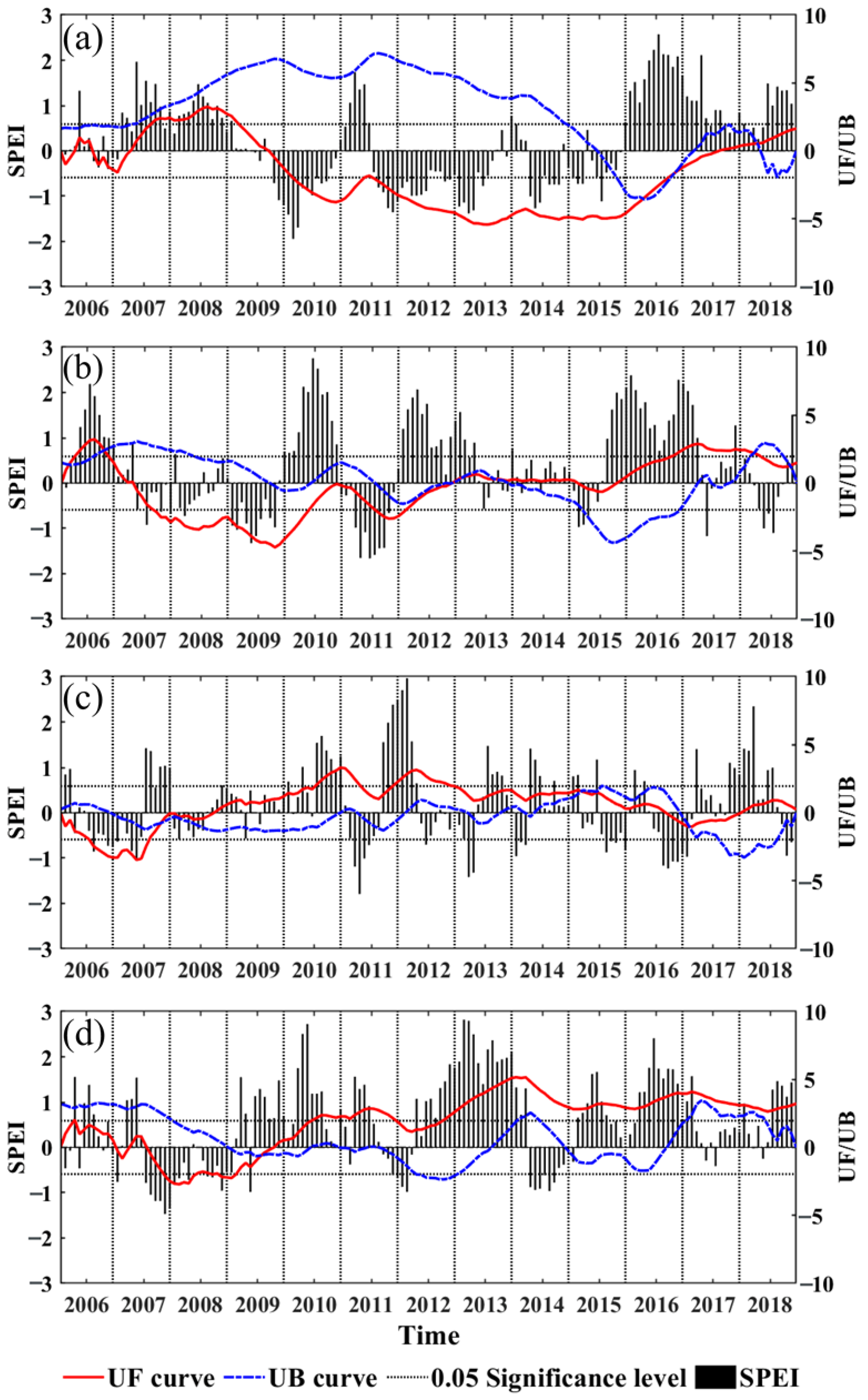
The Mann–Kendall test was performed on the SPEI values of the four provinces to analyze the time-series variation of SPEI in each province (Figure 2). In the years 2010, 2012, and 2014, the SPEI values of the Yunnan province were below the drought threshold. The trend test of the SPEI revealed (Figure 2a) that the UF curve of the SPEI was less than zero in the periods of early 2006, late 2016, early 2007, and 2009–2017, respectively. Additionally, the UF curve exceeded the 0.05 significance level line during 2010–2016, indicating that the SPEI in the Yunnan region had a significant decreasing trend and was prone to drought. Therefore, the drought stress from October 2009 to 2010 was studied in the Yunnan province to further analyze the performance characteristics of SIF, VIs, LAI, and fPAR during drought. The same analysis method determined the drought period from March to September 2018 for Fujian, February to August 2011 and May to December 2012 for the Shaanxi province, and July 2007 to December 2008 for the Heilongjiang province.

3.2. Response of SIF/SIFyield/VIs/LAI/fPAR to Drought Stress

3.2.1. Temporal Analysis

We analyzed the inter-annual variation of the standardized anomalies during drought for each of the variables (Figure 3). For the Yunnan province, the SIFyield responds promptly to drought, showing negative anomalies at the beginning of the drought in October 2009. From November 2009 to the end of 2010, the anomalies of SIF, NDVI, and EVI were all negative, which is consistent with the SPEIs indication of drought. LAI and fPAR showed negative anomalies in February 2010, indicating a more delayed response to drought. All the variables in the Shaanxi province showed the same result. For the Fujian province, only SIFyield showed negative anomalies. For the Heilongjiang province, all the variables synchronously reflected the negative anomalous changes, except for LAI and fPAR.
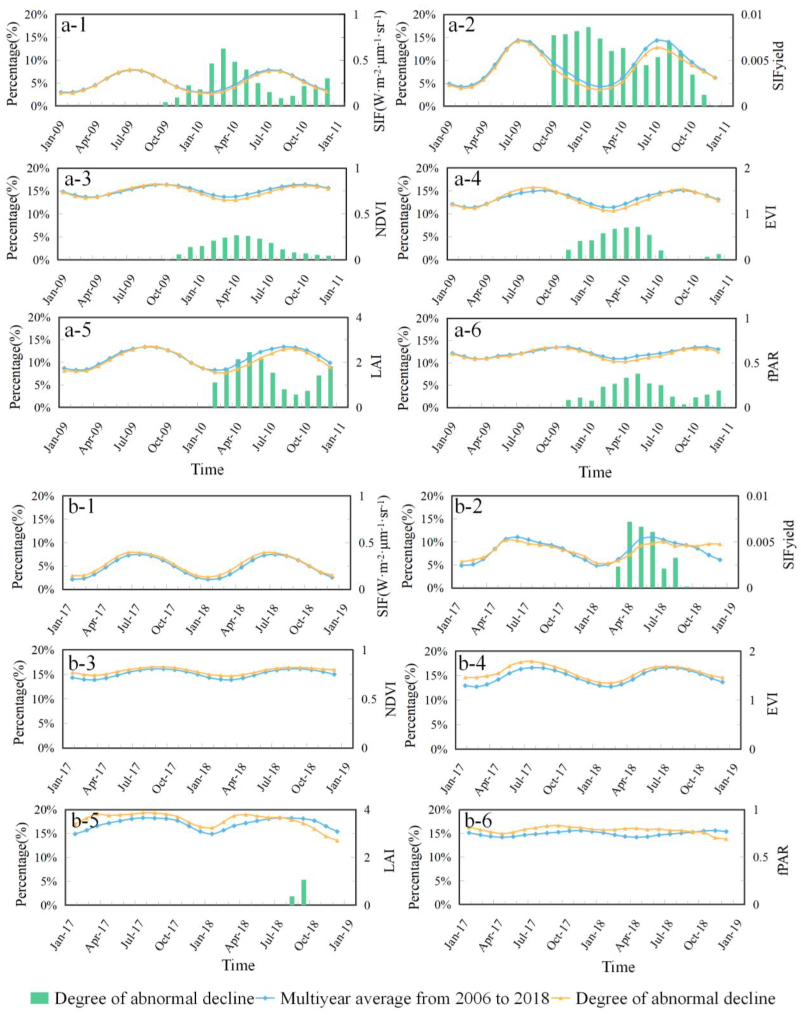
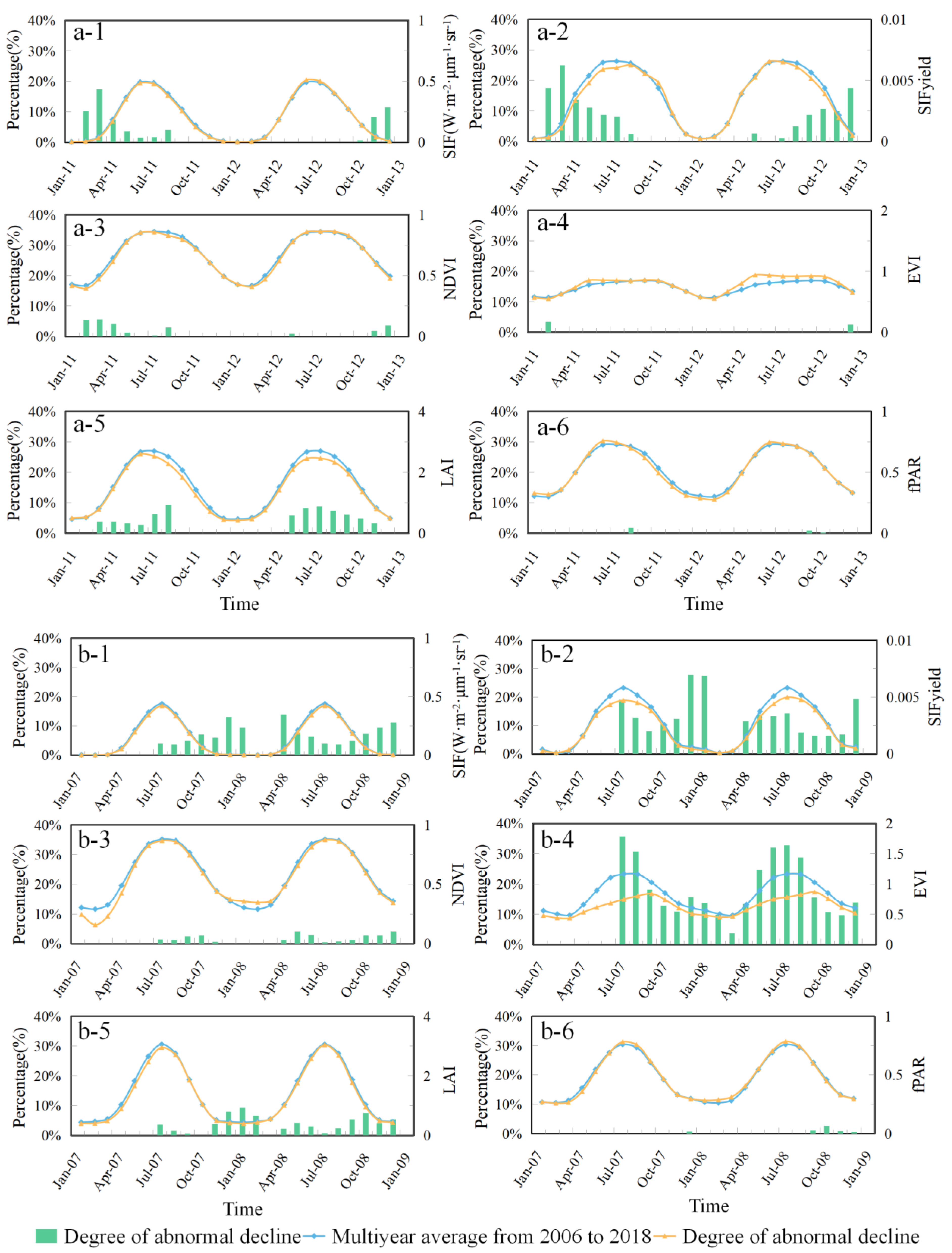
The seasonal cycle variation curves of SIF, SIFyield, VIs, LAI, and fPAR presented values and their multi-year averages are shown in Figure 4 and Figure 5. These variables exhibit a lower-than-average value during the drought, but the decline of several of them was different. The drought event in the Yunnan province showed that in October 2009, the regional SPEI value was −1.21, representing a moderate drought, and the decline in SIF, SIFyield, NDVI, EVI, LAI, and fPAR was 1.85%, 15.71%, 1.22%, 2.16%, 9.51%, and 1.88%, respectively. SIFyield had a larger descent range, suggesting that it was a better indicator of capturing early drought stress for forests. In June 2010, the SPEI value was −1.37, indicating that the drought condition was still severe. The declines in SIF, SIFyield, NDVI, EVI, LAI, and fPAR were 5.43%, 8.96%, 4.66%, 5.03%, 8.87%, and 5.39%, respectively. SIFyield showed the most significant decline. The degree of decline of the other variables was greater at this stage, indicating that the vegetation index responded more significantly in the middle and late stages of drought stress.
SIFyield also showed a more significant decline trend in the Shaanxi province, followed by SIF, LAI, and NDVI. Figure 4 also showed that only SIFyield responded to this drought event in Fujian, while the other variables failed to respond, highlighting the advantage of SIFyield for early drought stress monitoring. For the Heilongjiang province, the EVI value decreased by 35% in July 2007 compared to the multi-year average, being the indicator with the greatest decrease, followed by SIFyield with a 19% decrease.
To account for the impact of forest types, we compared the performances of the remote sensing variables (i.e., SIF, SIFyield, NDVI, EVI, LAI, and fPAR) in detecting drought over different forest types for each province. According to the vegetation regionalization map of China [35], Fujian is dominated by subtropical, evergreen broad-leaved forests. Yunnan is characterized by subtropical evergreen broad-leaved forests, tropical monsoon rainforests, and rainforests. Subtropical evergreen broad-leaved forests and warm-temperate deciduous broad-leaved forests are located in Shaanxi. Heilongjiang is distributed by cold-temperate coniferous forest and temperate coniferous and deciduous broad-leaved mixed forest. Thus, we performed comparisons over different forest types for Yunnan, Shaanxi, and Heilongjiang, respectively, and the resulting figures are shown in Appendix A.
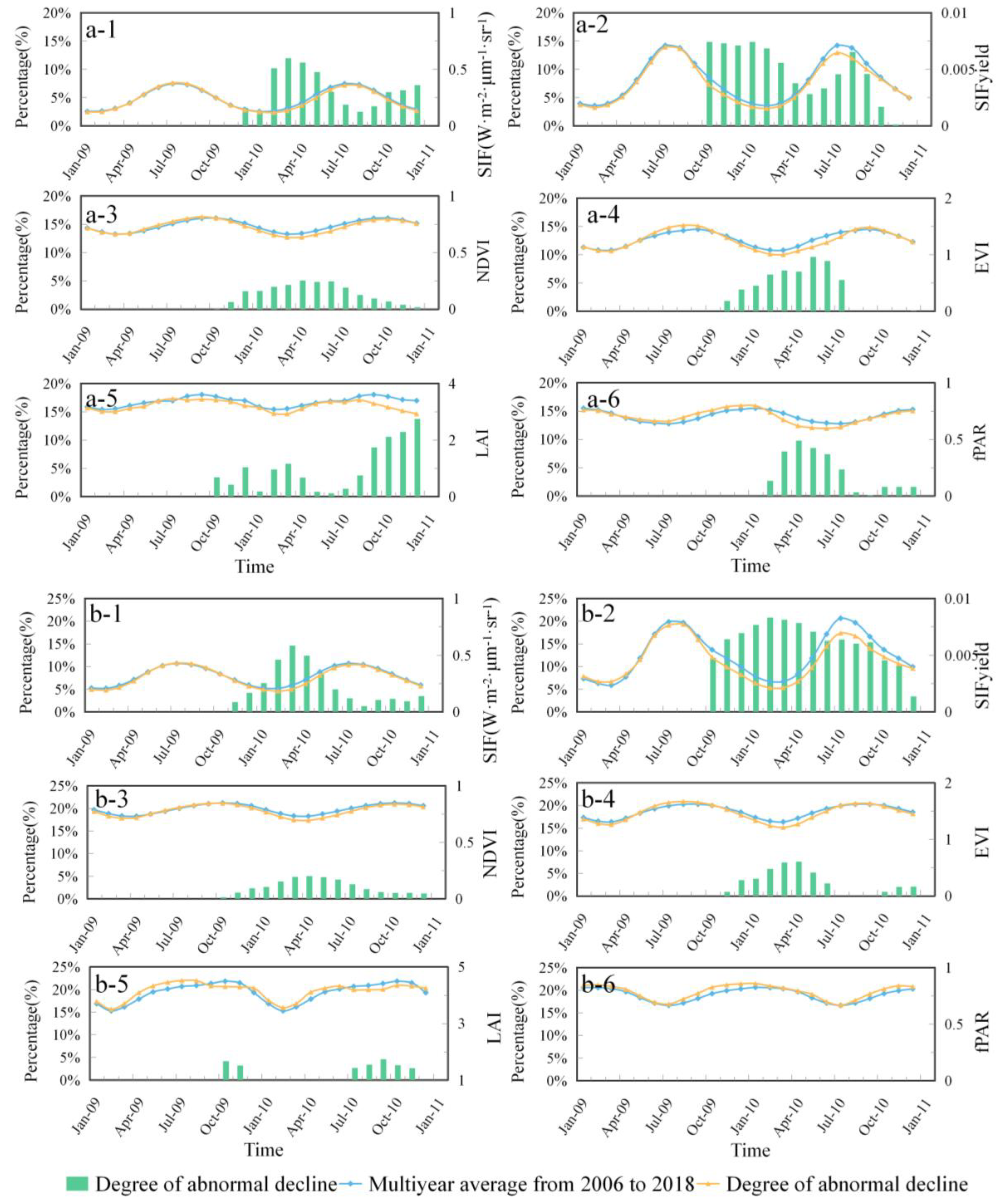
We found SIFyield showed significant decreases during the whole drought period for both subtropical evergreen broad-leaved forest and tropical monsoon rainforest, rainforest types of Yunnan province when compared with other variables, especially during the early drought period (Figure A1). In contrast, NDVI, EVI, and fPAR presented more decreases during the mid-drought period. Although SIF had a later decrease than SIFyield, its decrement was much earlier than other variables. Additionally, apart from SIFyield, SIF generally showed more decreases than other variables during the drought event, especially for the early drought period, indicating it is more sensitive to drought for both forest types over Yunnan province.
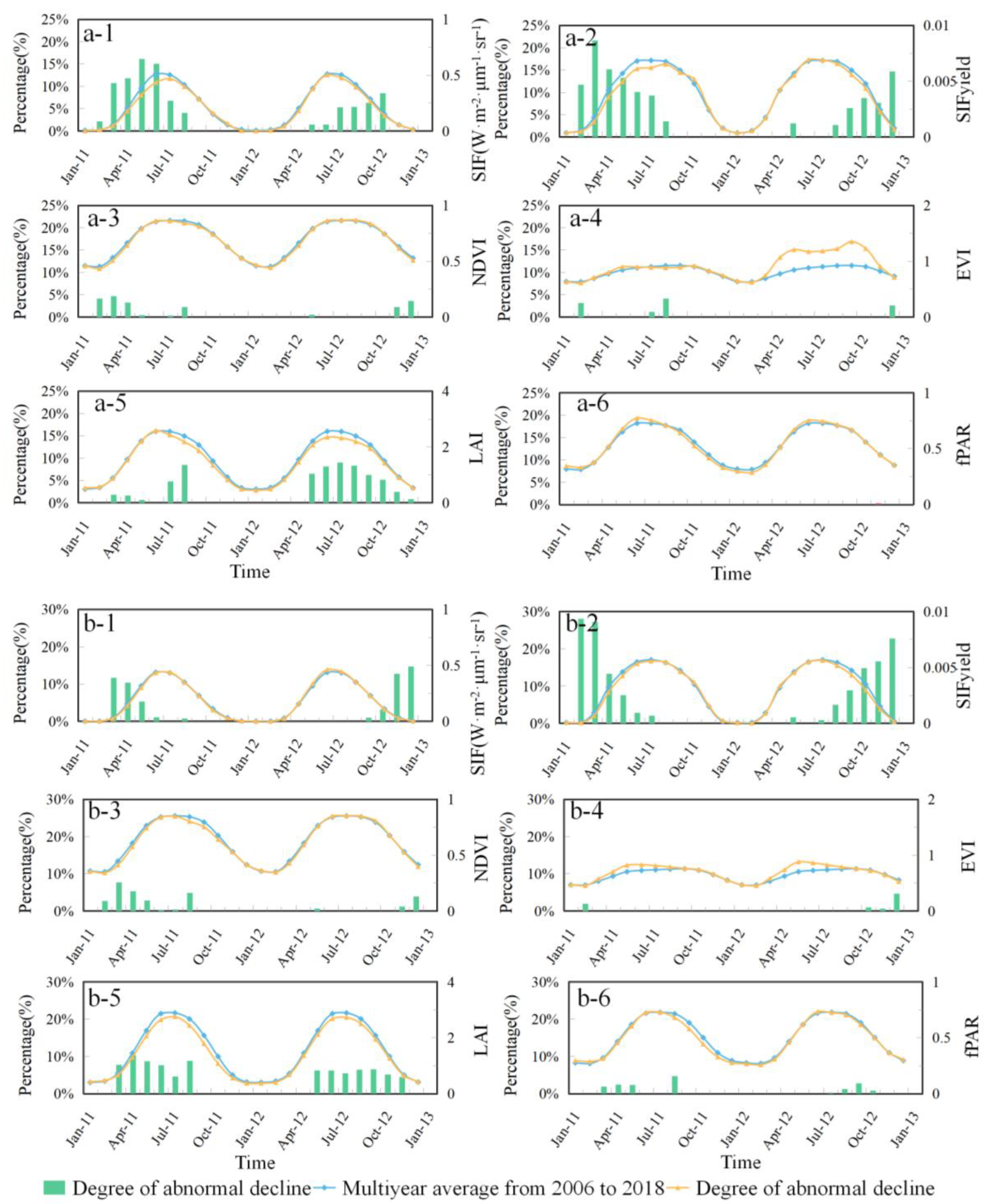
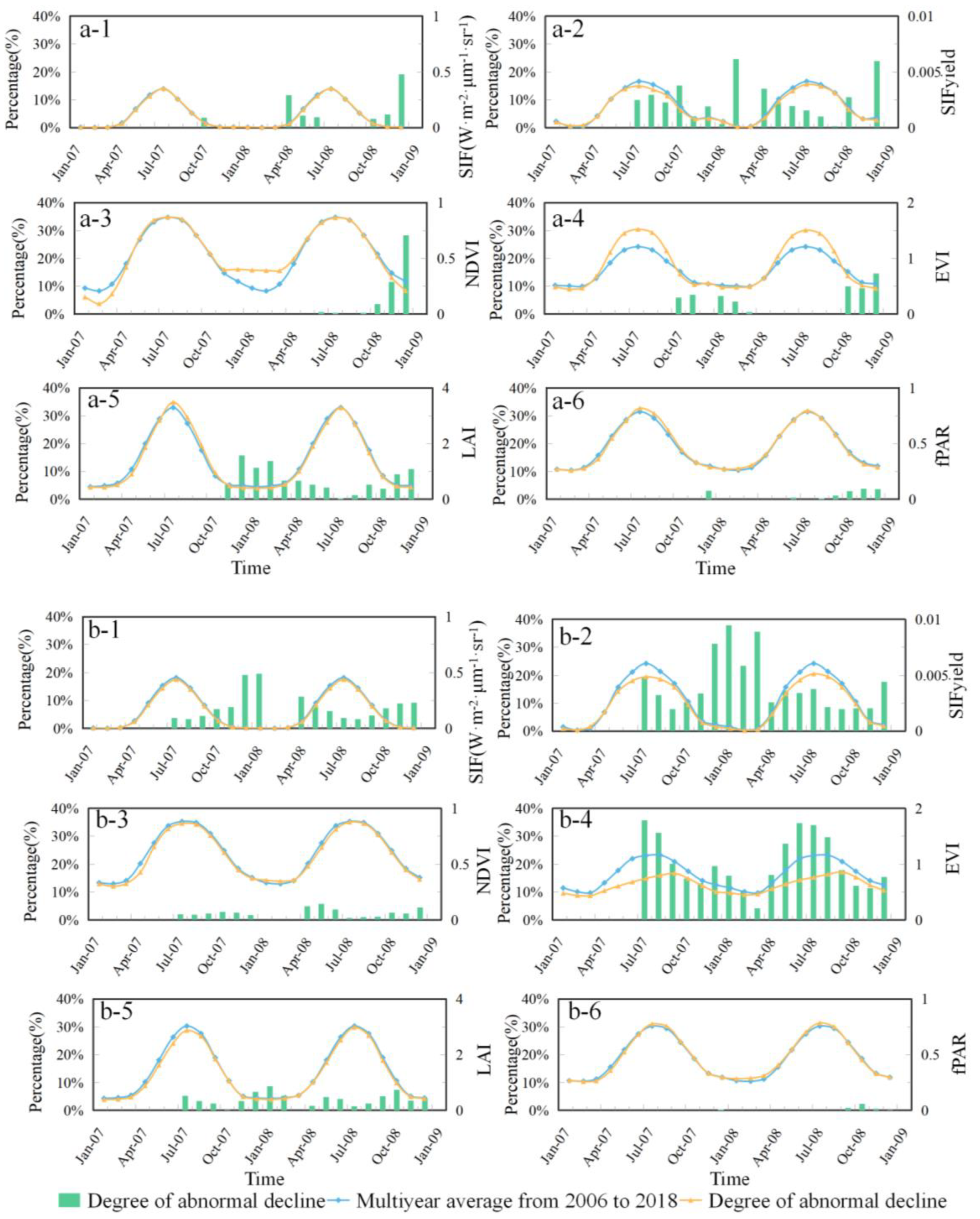
Figure A2 shows SIFyield decreased more for both subtropical evergreen broad-leaved forest and warm-temperate deciduous broad-leaved forests in Shaanxi during the drought event. SIF showed the next largest declines over the subtropical evergreen broad-leaved forest regions, while LAI presented more sensitivity to drought over the warm-temperate deciduous broad-leaved forest regions. For the Heilongjiang province, SIFyield outperformed other variables in capturing drought over the cold-temperate coniferous forest regions (Figure A3). By contrast, EVI showed more significant decreases over the temperate coniferous and deciduous broad-leaved mixed forest regions.

3.2.2. Spatial Analysis

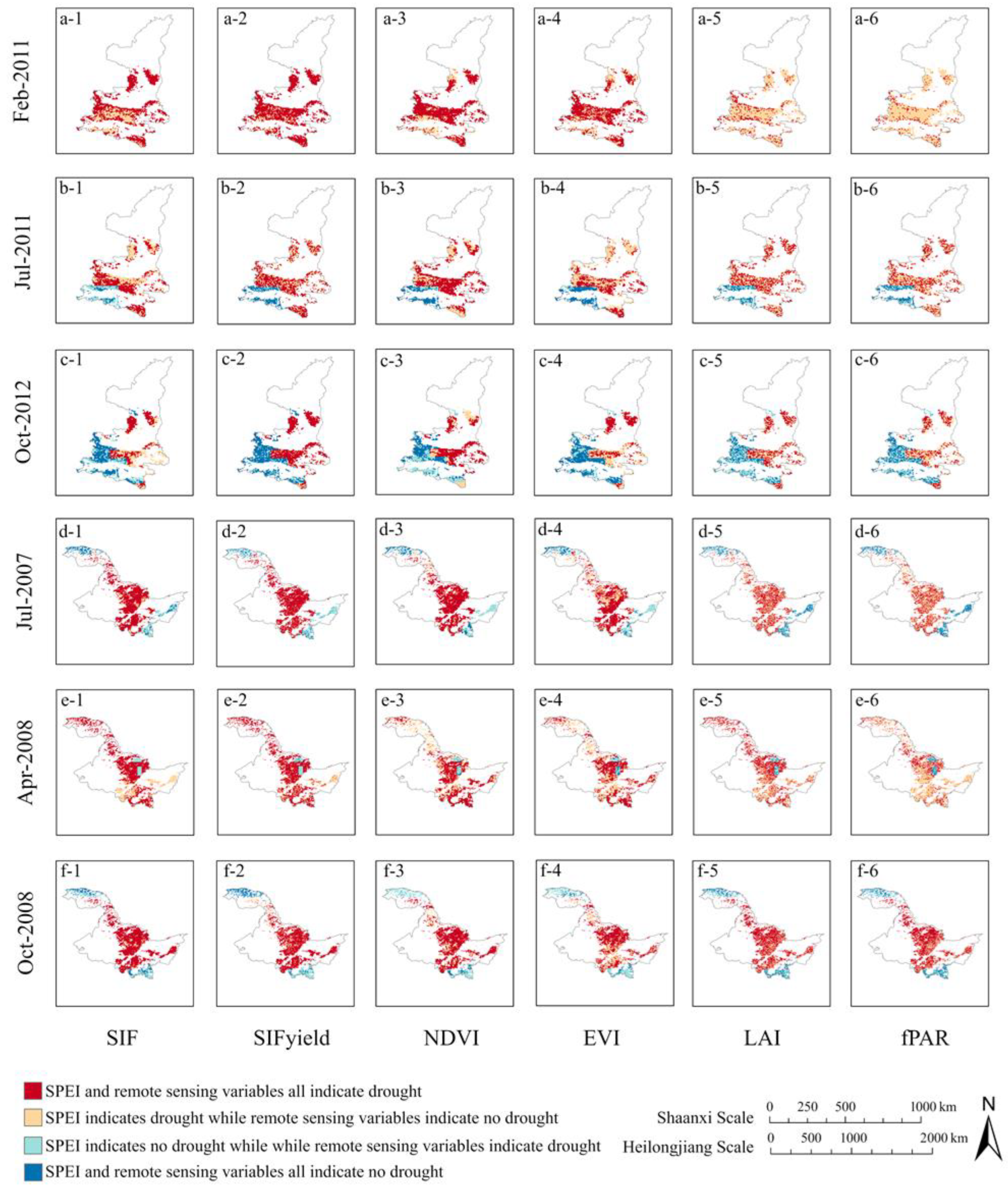
The spatial distribution of the standardized anomalies of SIF, SIFyield, VIs, LAI, and fPAR provides more information to study the dynamics of the forest’s response to drought stress. Figure 6 and Figure 7 depict the spatial distribution of each variable’s standardized anomalies in the four provinces at each stage of drought. Table 3 summarizes the percentage of drought areas indicated by SIF, SIFyield, VIs, LAI, and fPAR, respectively, which coincident with that indicated by the SPEI. For the Yunnan province, SIFyield showed a larger drought area that coincided with the drought regions detected by the SPEI at the early drought stage, followed by NDVI, EVI, LAI, and fPAR. At the middle and late stages of drought, NDVI showed a larger coincident region, which was consistent with the result that the vegetation indices responded more significantly in the middle and late stages of drought stress, as expressed in Section 3.2.1. Additionally, the drought conditions indicated by the SPEI were alleviated at the late drought stage in the northwestern part of Yunnan. Only SIFyield showed simultaneous easing near the central part of Yunnan, while the other variables still showed drought, suggesting the legacy effects of drought on forests.
For Shaanxi, the spatial extent of drought indicated by SIFyield also showed a larger coincident with that of the SPEI at the beginning of the drought. NDVI and SIFyield described a similar drought extent in the middle drought, but there were some differences in the spatial distribution. SIFyield showed drought relief in western and southern Shaanxi in the later period, while the other variables showed large drought legacy effects. For Fujian, only SIFyield showed coincident drought regions with the SPEI during the drought period. In contrast to the first two provinces, LAI and fPAR performed better than VIs in drought monitoring. For Heilongjiang, SIFyield showed the largest coincident drought regions during the drought period. Consequently, VIs, LAI, and fPAR behaved differently in different provinces, which may be related to the vegetation type and vegetation cover. Overall, SIFyield captured a greater spatial extent of drought for all four provinces, especially for the early detection of drought stress.

3.3. Correlation Analysis

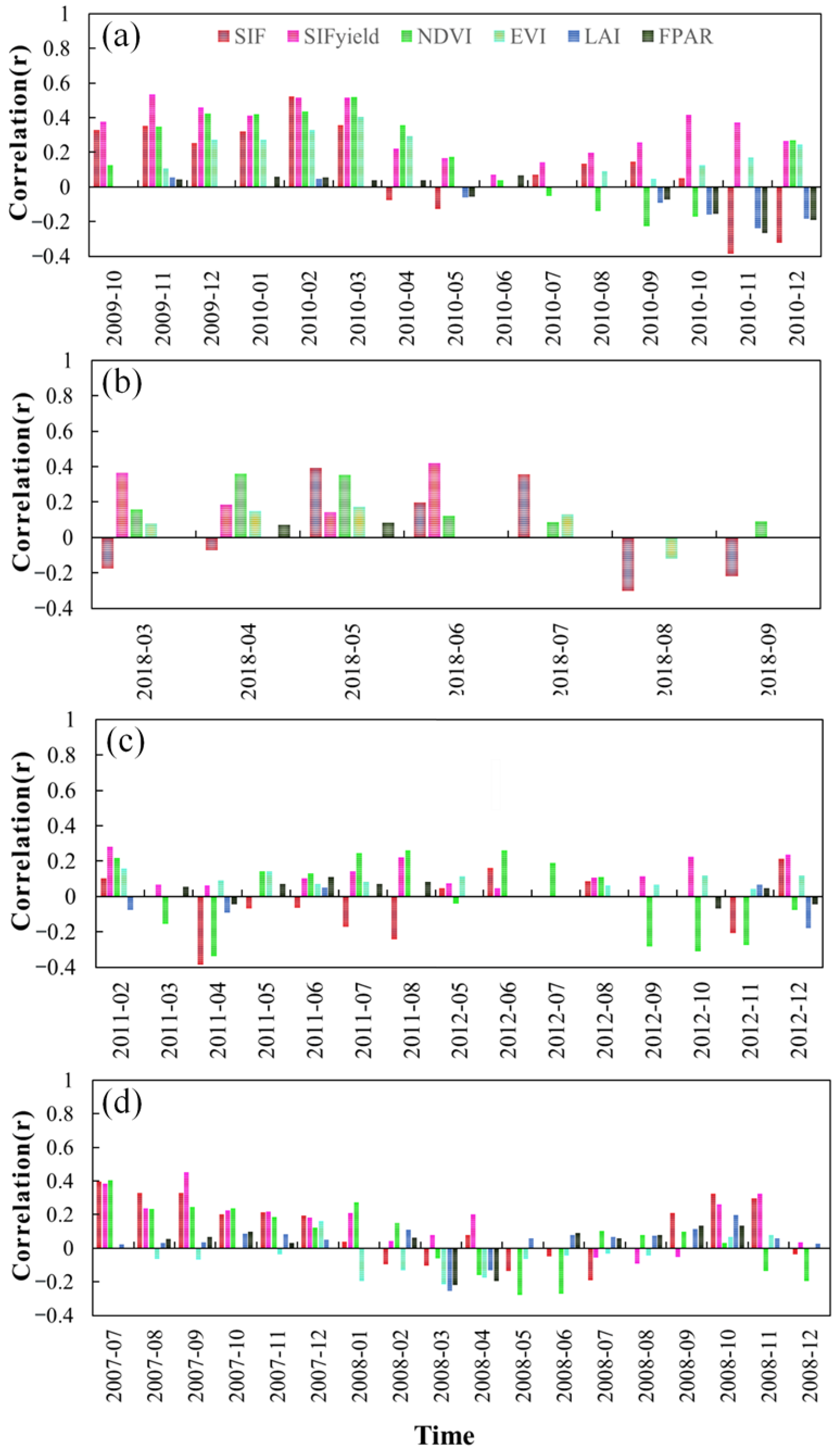
The correlations between SIF, SIFyield, NDVI, EVI, LAI, and fPAR with the SPEI for the four provinces were analyzed, and the correlation coefficients that passed the significance test (p < 0.05) are shown in Figure 8. In October 2009, the correlation coefficients of the standardized anomalies of the SIF, SIFyield, NDVI and SPEI in the Yunnan province were 0.33, 0.38, and 0.13, respectively; the correlation coefficients of SIF and SIFyield were higher than the vegetation indices. NDVI had the highest correlation with SPEI in March 2010 (r = 0.52), which was consistent with the spatial extent indicated in the Section 3.2.2 response results. When the drought eased, SIF and NDVI had varying degrees of delayed responses and a negative correlation with the SPEI, whereas SIFyield was always in a positive correlation. Moreover, the results showed that LAI and fPAR did not show an advantage throughout the drought period, and the correlations with the SPEI were either very low or negative.
For the Fujian province, more variables failed to pass the significance test, and SIFyield, NDVI, and SIF occupied the peak in March, April, and May, respectively. The correlation of variables in the Shaanxi province was generally lower, except SIFyield had the most amount of positively correlated months. The performance of variables in Heilongjiang was similar to that of Yunnan, and SIFyield showed the highest correlation.
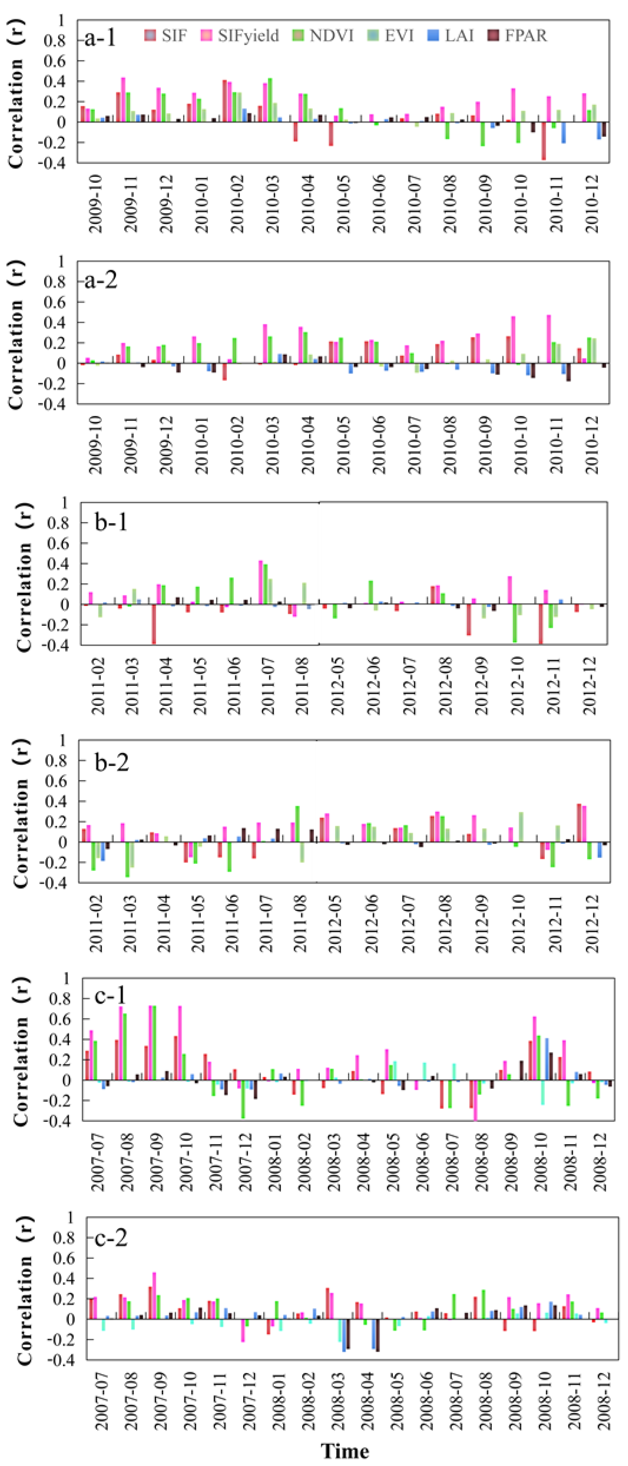
The correlations between the remote sensing variables and the SPEI over different forest types for each province were also assessed, as shown in Figure A4. Our results indicated that SIFyield had a significantly higher correlation with SPEI than the other variables in most cases (i.e., subtropical evergreen broad-leaved forests, tropical monsoon rainforests, and rainforests in Yunnan; subtropical evergreen broad-leaved forests and warm-temperate deciduous broad-leaved forests in Shaanxi; and cold-temperate coniferous forests in Heilongjiang). SIFyield was more correlated with SPEI during the whole drought period for both forest types in the Yunnan province and the cold-temperate coniferous forest region in the Heilongjiang province. Apart from SIFyield, SIF and NDVI generally showed higher correlations than the other variables. SIFyield, SIF, NDVI, and EVI in the cold-temperate coniferous forest regions showed higher correlations than under other forest types. Generally, the comparisons of the different forest types for each province highlighted the advantages of SIFyield in capturing drought in most cases.

3.4. Variable Importance Measurement Based on Random Forest

We deployed the pixels for the drought periods studied in four provinces to train the random forest model separately, with a total of 41,608 samples in Yunnan, 9114 samples in Fujian, 33,900 samples in Shaanxi, and 119,448 samples in Heilongjiang, respectively. The importance of each variable was identified by measuring its degree of influence on the accuracy of the model. It is the difference in the “Out of Bag” prediction error before and after permutation. A larger variable importance value indicates that mis-specification detracts from the predictive accuracy in the forests. A smaller variable importance value indicates that the variable contributes less to the predictive accuracy [59]. Figure 9 shows the importance in detecting drought for each remote sensing variable.
Our results showed that SIFyield was the most important variable in explaining the spatio-temporal distributions of SPEI value for all the provinces. This indicated that SIFyield was more closely related to the drought level indicated by the SPEI. SIF was the second most significant variable for the Yunnan, Fujian, and Heilongjiang provinces, followed by NDVI and EVI. We also found that LAI and fPAR were the least significant variables in detecting drought, indicating their limitations in drought monitoring. The assessment using the random forest algorithm confirmed that SIFyield outperformed the other variables in capturing drought, which was consistent with our findings in the spatio-temporal analysis.

4. Discussion

4.1. Temporal Analysis

The results of the four provincial studies suggest that SIFyield can effectively deliver more information about drought stress in the time scale. According to the Yearbook of Meteorological Disasters in China (2010), a global mega-drought occurred in southwest China, including Yunnan, from autumn 2009 to summer 2010 and 2011, which is consistent with the detection results based on the SPEI in this study. A region-wide drought occurred in Yunnan in October 2009, and the SIFyield response was one month earlier than the two vegetation indices and four months earlier than the LAI and fPAR. Moreover, SIFyield showed a more pronounced below-average phenomenon in the early stages of drought stress. Two rainfall processes occurred in Yunnan in late March and late April 2010, which reduced the extent of the drought, but the drought persisted in the severe drought areas until June [60]. As can be seen in Figure 3, only SIFyield reflected the drought mitigation in April, with a significant increase in the standardized anomaly. This indicates that SIFyield has an advantage in capturing both early drought and drought relief. In a study conducted by Liu et al. [61], the response of SIF to the drought events was also proved to be prompt, and the magnitude of decline was greater than that of NDVI, EVI, and NIRv.
For the Fujian province, only SIFyield responded to this drought stress. This may be attributed to the drought period in Fujian is shorter compared to the other three provinces. Li et al. [62] explained that the sensitivity of vegetation to short-term climate change in China has obvious spatial heterogeneity. Most of southwest China, parts of south-central China, and high-altitude mountainous areas in northwest and northeast China have high vegetation sensitivity. Among forest vegetation, high vegetation sensitivity occurs more often in mixed forests and alpine vegetation. Fujian belongs to the subtropical evergreen broad-leaved forest region, which is less sensitive to the climate. Lee et al. [63] used GOSAT SIF to monitor how seasonal water stress affects the Amazonian forest’s productivity. They concluded that plant photosynthesis was decreased by stomatal closure under short-term, mild drought events and returned to initial levels after the drought. SIF reflects vegetation photosynthesis, and VIs are based on surface information in estimating the drought degree of plants. Changes in vegetation conditions are triggered by the accumulation of weather conditions [64]. This may explain why VIs, LAI, and fPAR did not respond to this short-term drought event in Fujian province.
SIFyield, SIF, and NDVI responded to the stress onset synchronously during the 2011 drought period in the Shaanxi province, showing one month earlier than LAI and fPAR. In the 2012 drought period, SIFyield responded three months earlier than the other variables. SIFyield was also the most significant variable in terms of the magnitude of the decline in values during the drought. Moreover, only SIFyield did not show negative anomalies in the middle period of the two drought stresses, indicating its advantage in drought relief. SIFyield, SIF, and vegetation indices in the Heilongjiang province responded to drought stress synchronously and were three months earlier than LAI and fPAR. The value of EVI decreased most significantly during the drought. However, combined with the inter-annual trend of anomalies (Figure 3d), EVI was already in a negative anomaly before July 2007, i.e., when no drought stress occurred, and while SIFyield did not show a negative anomaly. Therefore, the dominance of EVI may not be scientifically valid.

4.2. Spatial Analysis

The spatial distribution of standardized anomalies enables us to obtain the differences in the spatial extent response of different variables and to analyze the differences in the response of each variable under drought stress in different periods. The range of the drought areas indicated by SIFyield synchronously with the SPEI in all four provinces was larger than that indicated by other variables, and it captured the spatial extent of drought more accurately. Pandiyan et al. [65] used data from 2007 to 2017 in the Heilongjiang and Jiangsu province of China to study drought events in 2015. Their results showed that SIF was more useful in spatially and temporally detecting droughts compared to LAI and NDVI. In our study, there were some areas, such as northern Yunnan, southern Shaanxi, and southern Heilongjiang, that did not respond to the drought in time, which can be attributed to the uncertainties of the SIF data. SIF obtained from satellite platforms is affected by various environmental factors, such as the atmospheric environment, observation angle, and solar altitude, making the relationship between SIFyield and water stress more complex [66]. The coarse spatial resolution of the SPEI dataset used in this study can also lead to uncertainties.
The monitoring ability of VIs differed significantly among the four provinces. For the Yunnan province, VIs described a larger area range than SIFyield when the drought was in the middle and late stages. This is consistent with the characterization results of Chen et al. [30], who found NDVI to be more sensitive to extreme drought in their drought monitoring of wheat in the Shandong province. Liu et al. [64] designed different drought intensity treatments on wheat plots with continuous ground observations of SIF and NDVI. Their results also indicated that NDVI was more feasible for longer drought durations. The Yunnan province showed the dominance of NDVI, probably because of the wide range of extreme drought events in Yunnan in 2009–2010, compared with the drought events in the other three provinces. The changes in plant characteristics (e.g., chlorophyll content and growth rate) under an extreme drought event can be reflected spectrally, leading to the responses of NDVI.
A vegetation water deficit can lead to a reduction in LAI and a corresponding reduction in fPAR, which is absorbed by the vegetation layer. Shekhar et al. [67] used OCO-2 solar-induced fluorescence to capture the effects of drought and high temperatures on different vegetation types in Europe in 2018. They found that compared to NDVI, SIF and fPAR had a faster response rate and possibly a higher sensitivity to drought. However, the LAI and fPAR data based on satellite remote sensing in our study performed differently in drought monitoring. The spatial distribution maps of the drought showed that only in the middle and late drought stages in Yunnan and Heilongjiang did LAI and fPAR reflect some negative regional anomalies. This is probably due to the higher vegetation sensitivity in Yunnan and Heilongjiang and the more severe drought in the Yunnan province. The satellite LAI and fPAR products are mainly based on vegetation reflectance information and are not the best variables to reflect vegetation physiological functions such as photosynthesis.

4.3. Correlation and Validation Analysis

In the correlation analysis with the drought indicator SPEI, the high correlation coefficient was not only related to the simultaneous indication of drought by SPEI and each variable, but it was also the simultaneous indication of wetness. The poor correlation detected in the forest areas may be explained by canopy complexity [68]. During the early drought period, the correlation of SIFyield was higher than that of other variables in all four provinces. During the late drought period, the drought area indicated by the SPEI became smaller. Although there was no severe meteorological drought in the study area, the cumulative effect of meteorological drought in the previous months caused the growth of regional vegetation to stagnate during the growing season. NDVI and EVI in most areas still showed negative anomalies. This is also in line with Anderegg et al. [69], who suggested that forests can exhibit the legacy effects of drought. They illustrated that the legacy effects of drought can last for 3 to 4 years, and slow growth and incomplete recovery of trees are common during this period. It also should be noted that the native spatial resolutions of the remote sensing variables are different in our study. For example, SPEI has a spatial resolution of 0.5°, which is much coarser than 0.05°. This coarse resolution and the nearest neighbor resampling performed can result in uncertainties in deriving drought and non-drought regions. Additionally, both LAI and fPAR have higher spatial resolutions than other datasets, which may lead to different drought detection results.
We deployed the random forest algorithm to assess remote sensing variables’ importance in monitoring drought. SIFyield ranks first in the variable importance of all provinces. It confirmed that SIFyield outperformed the other variables in capturing drought, which was consistent with our findings in the spatio-temporal analysis. It is worth noting that previous studies have shown that there is a linear correlation between SIF and vegetation indices (i.e., NDVI and EVI) [70]. Canopy SIF is also affected by LAI [71]. In addition, SIFyield is directly related to fPAR and SIF. These correlations may lead to uncertainties in the variable importance analysis with random forest. Further studies are still needed in evaluating the capacities of remote sensing variables in detecting drought using other machine learning algorithms.
Our study focused on the assessment of remote sensing variables (i.e., SIF, SIFyield, NDVI, EVI, LAI, and fPAR) for detecting drought. The results of our finding can support and provide references for further studies for detecting drought regions and/or drought durations using real-time remote sensing variables. We also found that the machine learning method presented potentials for capturing drought, which will provide a new perspective for accurately depicting drought events in the future.

5. Conclusions

In this paper, the different responses of SIF, SIFyield, VIs, LAI, and fPAR to drought conditions in the forest regions in the Yunnan, Fujian, Shaanxi, and Heilongjiang provinces in China were demonstrated. The application potential of these variables in drought stress monitoring was explored, and a random forest classification model was constructed to analyze the importance of SIF, SIFyield, VIs, LAI, and fPAR, which was validated against the analytical results. In general, SIFyield showed an earlier response to drought stress and had a larger descent range than other variables in all four provinces. On the spatial scale, SIFyield responded more significantly to mild drought stress and showed a greater spatial extent of drought. The correlation between SIFyield and the SPEI was higher in all four provinces during the drought period. In the late drought period, when other variables were mostly negatively related with SPEI, SIFyield still showed a higher correlation. The variable importance measurement based on the random forest classification algorithm also confirmed that SIFyield outperformed other variables (i.e., SIF, NDVI, EVI, LAI, and fPAR) in detecting drought. Therefore, it can be concluded that SIFyield is an effective tool for monitoring drought stress in different regions of China.

Author Contributions

Conceptualization, T.C. and L.C.; methodology, H.M. and T.C.; validation, H.M. and T.C.; formal analysis, H.M. and T.C.; resources, H.M. and T.C.; data curation, H.M. and T.C.; writing—original draft preparation, H.M.; writing—review and editing, H.M., T.C. and L.C.; visualization, H.M.; supervision, L.C.; funding acquisition, L.C. All authors have read and agreed to the published version of the manuscript.

Funding

This research was funded by the National Natural Science Foundation of China (31922055, 42201364) and the Priority Academic Program Development of Jiangsu Higher Education Institutions (PAPD), the natural Science Foundation of Jiangsu Province (BK20190764), and the Open Fund of State Key Laboratory of Remote Sensing Science (OFSLRSS202005).

Acknowledgments

The authors gratefully acknowledge the graduate students from the department of forest management at Nanjing Forestry University for providing suggestions for improving this study.

Conflicts of Interest

The authors declare no conflict of interest.

Appendix A

Figure A1. (a1a6) The seasonal cycle variation curves of present values and multi-year averages and the abnormal decrease amplitude of the present values from the average values of SIF, SIFyield, NDVI, EVI, LAI, and fPAR, respectively, of the subtropical evergreen broad-leaved forest region in Yunnan province (b1b6). The seasonal cycle variation curves of present values and multi-year averages and the abnormal decrease amplitude of the present values from the average values of SIF, SIFyield, NDVI, EVI, LAI, and fPAR, respectively, of the tropical monsoon rainforest and rainforest region in Yunnan province.
Remotesensing 15 00879 g0a1
Figure A2. (a1a6) The seasonal cycle variation curves of present values and multi-year averages and the abnormal decrease amplitude of the present values from the average values of SIF, SIFyield, NDVI, EVI, LAI, and fPAR, respectively, of the subtropical evergreen broad-leaved forest region in Shaanxi province (b1b6). The seasonal cycle variation curves of present values and multi-year averages and the abnormal decrease amplitude of the present values from the average values of SIF, SIFyield, NDVI, EVI, LAI, and fPAR, respectively, of the warm-temperate deciduous broad-leaved forest region in Shaanxi province.
Remotesensing 15 00879 g0a2
Figure A3. (a1a6) The seasonal cycle variation curves of present values and multi-year averages and the abnormal decrease amplitude of the present values from the average values of SIF, SIFyield, NDVI, EVI, LAI, and fPAR, respectively, of the cold-temperate coniferous forest region in Heilongjiang province (b1b6). The seasonal cycle variation curves of present values and multi-year averages and the abnormal decrease amplitude of the present values from the average values of SIF, SIFyield, NDVI, EVI, LAI, and fPAR, respectively, of the temperate coniferous and deciduous broad-leaved mixed forest region in Heilongjiang province.
Remotesensing 15 00879 g0a3
Figure A4. Correlation between standardized anomalies of SIF, SIFyield, NDVI, EVI, LAI, and fPAR with SPEI. (a-1) the subtropical evergreen broad-leaved forest region in Yunnan province; (a-2) the tropical monsoon rainforest and rainforest region in Yunnan province; (b-1) the subtropical evergreen broad-leaved forest region in Shaanxi province; (b-2) the warm-temperate deciduous broad-leaved forest region in Shaanxi province; (c-1) the cold-temperate coniferous forest region in Heilongjiang province; (c-2) and the temperate coniferous and deciduous broad-leaved mixed forest region in Heilongjiang province.
Remotesensing 15 00879 g0a4

References

  1. Latif, M.; Sun, J.; Visbeck, M.; Hadi Bordbar, M. Natural variability has dominated Atlantic Meridional Overturning Circulation since 1900. Nat. Clim. Change 2022, 12, 455–460. [Google Scholar] [CrossRef]
  2. Grant, P.R. Evolution, climate change, and extreme events. Science 2017, 357, 451–452. [Google Scholar] [CrossRef]
  3. Su, J.; Wen, M.; Ding, Y.; Gao, Y.; Song, Y. Hiatus of global warming: A review. Chin. J. Atmos. Sci. 2016, 40, 1143–1153. [Google Scholar] [CrossRef]
  4. Wang, J.; Li, Y.; Wang, Y.; Feng, J.; Zhao, Y. Preliminary Analysis on the Demand and Review of Progress in the Field of Meteorological Drought Research. J. Arid Meteorol. 2012, 30, 497–508. [Google Scholar]
  5. Wang, Z.; Duan, M. Research Progress of Economic Losses Assessment in Drought Disaster in China. J. Anhui Agric. Sci. 2015, 43, 115–117. [Google Scholar] [CrossRef]
  6. Hammond, W.M.; Williams, A.P.; Abatzoglou, J.T.; Adams, H.D.; Klein, T.; López, R.; Sáenz-Romero, C.; Hartmann, H.; Breshears, D.D.; Allen, C.D. Global field observations of tree die-off reveal hotter-drought fingerprint for Earth’s forests. Nat. Commun. 2022, 13, 1761. [Google Scholar] [CrossRef] [PubMed]
  7. Forzieri, G.; Dakos, V.; McDowell, N.G.; Ramdane, A.; Cescatti, A. Emerging signals of declining forest resilience under climate change. Nature 2022, 608, 534–539. [Google Scholar] [CrossRef]
  8. Hansen, M.; Potapov, P.; Moore, R.; Hancher, M. High-Resolution Global Maps of 21st-Century Forest Cover Change. Science 2013, 342, 850–853. [Google Scholar] [CrossRef]
  9. McDowell, N.; Pockman, W.T.; Allen, C.D.; Breshears, D.D. Mechanisms of plant survival and mortality during drought: Why do some plants survive while others succumb to drought? New Phytol. 2008, 178, 719–739. [Google Scholar] [CrossRef]
  10. Choat, B.; Jansen, S.; Brodribb, T.J.; Cochard, H.; Delzon, S.; Bhaskar, R.; Bucci, S.J.; Feild, T.S.; Gleason, S.M.; Hacke, U.G.; et al. Global convergence in the vulnerability of forests to drought. Nature 2012, 491, 752–755. [Google Scholar] [CrossRef]
  11. Stovall, A.E.L.; Shugart, H.; Yang, X. Tree height explains mortality risk during an intense drought. Nat. Commun. 2019, 10, 4385. [Google Scholar] [CrossRef] [Green Version]
  12. Qian, X. A Vegetation Drought Stress Index Based on Solar-induced Chlorophyll Fluorescence; Nanjing University: Nanjing, China, 2019; p. 88. [Google Scholar]
  13. Chen, H.; Sun, J. Changes in Drought Characteristics over China Using the Standardized Precipitation Evapotranspiration Index. J. Clim. 2015, 28, 5430–5447. [Google Scholar] [CrossRef]
  14. Yuan, W.; Zhou, G. Theoratical Study and Research Prospect on Drought Indices. Adv. Earth Sci. 2004, 19, 982–991. [Google Scholar]
  15. Zhang, Q.; Yao, Y.; Li, Y.; Huang, J.; Ma, Z.; Wang, Z.; Wang, S.; Wang, Y.; Zhang, Y. Progress and prospect on the study of causes and variation regularity of droughts in China. Acta Meteorol. Sin. 2020, 78, 500–521. [Google Scholar] [CrossRef]
  16. Li, Q.; Zhu, J.; Feng, Y.; Xiao, W. Carbon Stocks and Carbon Sequestration Capacity of the Main Plantations in China. J. Northwest For. Univ. 2016, 31, 1–6. [Google Scholar] [CrossRef]
  17. Hou, X.; Zhao, J.; Zhao, H.; Ta, Z.; Yue, C. Drought effects on forest greenness anomalies in China from 2003 to 2018. China Environ. Sci. 2022, 42, 336–344. [Google Scholar] [CrossRef]
  18. Li, Y.; Li, Y. Advances in Adaptability of Meteorological Drought Indices in China. J. Arid Meteorol. 2017, 35, 709–723. [Google Scholar]
  19. Vicente-Serrano, S.M.; Beguería, S.; López-Moreno, J.I. A Multiscalar Drought Index Sensitive to Global Warming: The Standardized Precipitation Evapotranspiration Index. J. Clim. 2010, 23, 1696–1718. [Google Scholar] [CrossRef]
  20. Li, Y. Spatiotemporal Characterisation of Drought in Jilin Province Based on Meteorological Data and LST-NDVI Feature Space; Northeast Normal University: Jilin, China, 2015; p. 65. [Google Scholar]
  21. Wang, X. Construction and Application of Standardized Vegetation Moisture Index in Northeast China; Northwest Normal University: Gansu, China, 2021; p. 98. [Google Scholar]
  22. Ni, Z.; Huo, H.; Tang, S.; Li, Z.; Liu, Z.; Xu, S.; Chen, B. Assessing the response of satellite sun-induced chlorophyll fluorescence and MODIS vegetation products to soil moisture from 2010 to 2017: A case in Yunnan Province of China. Int. J. Remote Sens. 2019, 40, 2278–2295. [Google Scholar] [CrossRef]
  23. Ni, Z.; Liu, Z.; Huo, H.; Li, Z.; Nerry, F.; Wang, Q.; Li, X. Early Water Stress Detection Using Leaf-Level Measurements of Chlorophyll Fluorescence and Temperature Data. Remote Sens. 2015, 7, 3232–3249. [Google Scholar] [CrossRef]
  24. Zhang, Z.; Wang, S.; Qiu, B.; Song, L.; Zhang, Y. Retrieval of sun-induced chlorophyll fluorescence and advancements in carbon cycle application. J. Remote Sens. 2019, 23, 37–52. [Google Scholar] [CrossRef]
  25. Mohammed, G.H.; Colombo, R.; Middleton, E.M.; Rascher, U.; van der Tol, C.; Nedbal, L.; Goulas, Y.; Pérez-Priego, O.; Damm, A.; Meroni, M.; et al. Remote sensing of Solar-induced chlorophyll fluorescence (SIF) in vegetation: 50 years of progress. Remote Sens. Environ. 2019, 231, 111177. [Google Scholar] [CrossRef]
  26. Frankenberg, C.; Fisher, J.B.; Worden, J.; Badgley, G.; Saatchi, S.S.; Lee, J.; Toon, G.C.; Butz, A.; Jung, M.; Kuze, A.; et al. New global observations of the terrestrial carbon cycle from GOSAT: Patterns of plant fluorescence with gross primary productivity. Geophys. Res. Lett. 2011, 38. [Google Scholar] [CrossRef] [Green Version]
  27. Joiner, J.; Yoshida, Y.; Vasilkov, A.P.; Middleton, E.M.; Campbell, P.K.E.; Kuze, A.; Corp, L.A. Filling-in of far-red and near-Infrared solar lines by terrestrial and atmospheric effects: Simulations and space-based observations from SCIAMACHY and GOSAT. Atmos. Meas. Tech. Discuss. 2012, 5, 163–210. [Google Scholar] [CrossRef]
  28. Kohler, P.; Guanter, L.; Frankenberg, C. Simplified physically based retrieval of sun-induced chlorophyll fluorescence from GOSAT data. IEEE Geosci. Remote Sens. Lett. 2015, 12, 1446–1450. [Google Scholar] [CrossRef]
  29. Wang, S.; Huang, C.; Zhang, L.; Lin, Y.; Cen, Y.; Wu, T. Monitoring and Assessing the 2012 Drought in the Great Plains: Analyzing Satellite-Retrieved Solar-Induced Chlorophyll Fluorescence, Drought Indices, and Gross Primary Production. Remote Sens. 2016, 8, 61. [Google Scholar] [CrossRef]
  30. Chen, X.; Ji, L.; Yu, K.; Zhao, Y. Monitoring of Drought in Shandong Province by Sun-induced Chlorophyll Fluorescence. China Sci. 2021, 16, 564–570. [Google Scholar]
  31. Sun, Y.; Fu, R.; Dickinson, R.; Joiner, J.; Frankenberg, C.; Gu, L.; Xia, Y.; Fernando, N. Drought onset mechanisms revealed by satellite solar-induced chlorophyll fluorescence: Insights from two contrasting extreme events. J. Geophys. Res. Biogeosci. 2015, 120, 2427–2440. [Google Scholar] [CrossRef]
  32. Yoshida, Y.; Joiner, J.; Tucker, C.; Berry, J.; Lee, J.E.; Walker, G.; Reichle, R.; Koster, R.; Lyapustin, A.; Wang, Y. The 2010 Russian drought impact on satellite measurements of solar-induced chlorophyll fluorescence: Insights from modeling and comparisons with parameters derived from satellite reflectances. Remote Sens. Environ. 2015, 166, 163–177. [Google Scholar] [CrossRef]
  33. Xu, S.; Liu, Z.; Zhao, L.; Zhao, H.; Ren, S. Diurnal Response of Sun-Induced Fluorescence and PRI to Water Stress in Maize Using a Near-Surface Remote Sensing Platform. Remote Sens. 2018, 10, 1510. [Google Scholar] [CrossRef]
  34. Ma, P.; Han, L.; Zhang, X.; Liu, W. Regional Characteristics of Drought in China under the Background of Climate Warming. J. Desert Res. 2019, 39, 209–215. [Google Scholar]
  35. Wu, Z. Chinese Vegetation; Science Press: Beijing, China, 1980; p. 1. [Google Scholar]
  36. Zhou, H.; Sun, H.; Shi, Z.; Peng, F.; Lin, Y. Solar-induced chlorophyll fluorescence data-based study on the spatial and temporal patterns of vegetation phenology in the Northern Hemisphere during the period of 2007–2018. J/OL. Remote Sens. 2021. [Google Scholar] [CrossRef]
  37. Pu, J.; Huang, Z.; Gao, M. Relationship between climatic characteristics and planting suitability of main cash crops in Yunnan. J. Meteorol. Res. 2021, 42, 53–57. [Google Scholar] [CrossRef]
  38. Zhang, W.; Zheng, J.; Ren, J. Climate Characteristics of Extreme Drought Events in Yunnan. J. Catastrophology 2013, 28, 59–64. [Google Scholar] [CrossRef]
  39. Zhang, R.; Zhuang, Y.; Xue, F.; Chen, S.; Lin, X.; Pan, H. Monitoring, Early-Warming and Assessment Techniques of Meteorological Drought Risk in Fujian Province. J. Catastrophology 2019, 34, 114–122. [Google Scholar] [CrossRef]
  40. Cai, X.; Wu, S.; He, H.; Jiang, C.; Sun, X.; Gao, H.; Zheng, G. Change of Extreme Climate Events in Shaanxi Province under Global Warming Background. J. Desert Res. 2012, 32, 1095–1101. [Google Scholar]
  41. Wang, Z.; Sun, C.; Liu, Y.; Jiang, Q.; Zhu, T. Spatiotemporal variation of vegetation index and its response to climate factors in Heilongjiang Province. South-North Water Transf. Water Sci. Technol. 2022, 20, 737–747. [Google Scholar] [CrossRef]
  42. Friedl, M.A.; Sulla-Menashe, D.; Tan, B.; Schneider, A.; Ramankutty, N.; Sibley, A.; Huang, X.M. MODIS Collection 5 global land cover: Algorithm refinements and characterization of new datasets. Remote Sens. Environ. Interdiscip. J. 2010, 114, 168–182. [Google Scholar] [CrossRef]
  43. Vicente-Serrano, S.M.; Beguería, S.; López-Moreno, J.I.; Angulo, M.; Kenawy, A.E. A New Global 0.5° Gridded Dataset (1901–2006) of a Multiscalar Drought Index: Comparison with Current Drought Index Datasets Based on the Palmer Drought Severity Index. J. Hydrometeorol. 2010, 11, 1033–1043. [Google Scholar] [CrossRef]
  44. Beguería, S.; Vicente-Serrano, S.M.; Angulo-Martínez, M. A Multiscalar Global Drought Dataset: The SPEIbase: A New Gridded Product for the Analysis of Drought Variability and Impacts. Bull. Am. Meteorol. Soc. 2010, 91, 1351–1356. [Google Scholar] [CrossRef]
  45. Yang, S.; Meng, D.; Li, X.; Wu, X. Multi-scale responses of vegetation changes relative to the SPEI meteorological drought index in North China in 2001–2014. Acta Ecol. Sin. 2018, 38, 1028–1039. [Google Scholar]
  46. Muñoz Sabater, J. ERA5-Land Monthly Averaged Data from 1981 to Present. Copernicus Climate Change Service (C3S) Climate Data Store (CDS). 2019. Available online: https://cds.climate.copernicus.eu/cdsapp#!/dataset/reanalysis-era5-land-monthly-means?tab=form (accessed on 28 December 2021).
  47. Papaioannou, G.; Papanikolaou, N.; Retalis, D. Relationships of photosynthetically active radiation and shortwave irradiance. Appl. Clim. 1993, 48, 23–27. [Google Scholar] [CrossRef]
  48. Schaaf, C.; Wang, Z. MCD43C4 MODIS/Terra+Aqua BRDF/Albedo Nadir BRDF-Adjusted Ref Daily L3 Global 0.05Deg CMG V061 2021, Distributed by NASA EOSDIS Land Processes DAAC. Available online: https://lpdaac.usgs.gov/products/mcd43c4v061 (accessed on 28 December 2021).
  49. Myneni, R.; Knyazikhin, Y.; Park, T. MOD15A2H MODIS/Terra Leaf Area Index/FPAR 8-Day L4 Global 500m SIN Grid V006 2015, distributed by NASA EOSDIS Land Processes DAAC. Available online: https://lpdaac.usgs.gov/products/mod15a2hv006 (accessed on 28 December 2021).
  50. Li, X.; Xiao, J. A Global, 0.05-Degree Product of Solar-Induced Chlorophyll Fluorescence Derived from OCO-2, MODIS, and Reanalysis Data. Remote Sens. 2019, 11, 517. [Google Scholar] [CrossRef]
  51. Luo, X.; Li, Y.; Yin, H.; Sui, M. Response of NDVl to SPEl at different temporal scales in Northeast China. Chin. J. Ecol. 2020, 39, 412–421. [Google Scholar] [CrossRef]
  52. GB/T 20481-2017; Grades of Meteorological Drought. China Meteorological Administration: Beijing, China, 2017.
  53. Tang, J. Analysis of precipitation characteristics of the last 55 years in the Tianshan Mountains based on MK test. Gansu Water Resour. Hydropower 2019, 55, 5–8. [Google Scholar] [CrossRef]
  54. Cao, J.; Chi, D.; Wu, L.; Liu, L.; Li, S.; Yu, M. Mann-Kendall Examination and Application in the Analysis of Precipitation Trend. Agric. Sci. Technol. Equip. 2008, 5, 35–37. [Google Scholar] [CrossRef]
  55. Breiman, L. Random forests—Random features. Mach. Learn. 2001, 45, 5–32. [Google Scholar] [CrossRef] [Green Version]
  56. Mitchell, M.W. Bias of the Random Forest Out-of-Bag (OOB) Error for Certain Input Parameters. Open J. Stat. 2011, 01, 205–211. [Google Scholar] [CrossRef]
  57. Nicodemus, K.K. Letter to the editor: On the stability and ranking of predictors from random forest variable importance measures. Brief. Bioinform. 2011, 12, 369–373. [Google Scholar] [CrossRef]
  58. Song, S.; He, R. lmportance measure index system based on random forest. J. Natl. Univ. Def. Technol. 2021, 43, 25–32. [Google Scholar] [CrossRef]
  59. Jiao, W.; Chang, Q.; Wang, L. The Sensitivity of Satellite Solar-Induced Chlorophyll Fluorescence to Meteorological Drought. Earth’s Future 2019, 7, 558–573. [Google Scholar] [CrossRef]
  60. Peng, G.; Liu, Y. A Dynamic Risk Analysis of 2009—2010 Yunnan Extra-Severe Drought. Adv. Meteorol. Sci. Technol. 2012, 2, 50–52. [Google Scholar] [CrossRef]
  61. Liu, Q.; Zhang, F.; Zhao, X. The superiority of solar-induced chlorophyll fluorescence sensitivity over other vegetation indices to drought. J Arid Environ. 2022, 204, 104787. [Google Scholar] [CrossRef]
  62. Li, X. Development and Application of a LAl-Based Global Vegetation Drought Index; Tsinghua University: Beijing, China, 2017; p. 81. [Google Scholar]
  63. Lee, J.; Frankenberg, C.; van der Tol, C.; Berry, J.A.; Guanter, L.; Boyce, C.K.; Fisher, J.B.; Morrow, E.; Worden, J.R.; Asefi, S.; et al. Forest productivity and water stress in Amazonia: Observations from GOSAT chlorophyll fluorescence. Proc. R. Soc. B Biol. Sci. 2013, 280, 20130171. [Google Scholar] [CrossRef]
  64. Liu, L.; Yang, X.; Zhou, H.; Liu, S.; Zhou, L.; Li, X.; Yang, J.; Han, X.; Wu, J. Evaluating the utility of solar-induced chlorophyll fluorescence for drought monitoring by comparison with NDVI derived from wheat canopy. Sci. Total Environ. 2018, 625, 1208–1217. [Google Scholar] [CrossRef]
  65. Pandiyan, S.; Govindjee, G.; Meenatchi, S.; Prasanna, S.; Gunasekaran, G.; Guo, Y. Evaluating the Impact of Summer Drought on Vegetation Growth Using Space-Based Solar-Induced Chlorophyll Fluorescence Across Extensive Spatial Measures. Big Data 2022, 10, 230–245. [Google Scholar] [CrossRef]
  66. Liu, Z.; Wu, J.; Zhou, H.; Li, X.; Wang, Q.; An, X.; Li, R. Chlorophyll Fluorescence and lts Progress in Detecting Water Stress. Spectrosc. Spect. Anal. 2017, 37, 2780–2787. [Google Scholar]
  67. Shekhar, A.; Chen, J.; Bhattacharjee, S.; Buras, A.; Castro, A.O.; Zang, C.S.; Rammig, A. Capturing the Impact of the 2018 European Drought and Heat across Different Vegetation Types Using OCO-2 Solar-Induced Fluorescence. Remote Sens. 2020, 12, 3249. [Google Scholar] [CrossRef]
  68. Guo, M.; Li, J.; Huang, S.; Wen, L. Feasibility of Using MODIS Products to Simulate Sun-Induced Chlorophyll Fluorescence (SIF) in Boreal Forests. Remote Sens. 2020, 12, 680. [Google Scholar] [CrossRef]
  69. Anderegg, W.R.; Schwalm, C.; Biondi, F.; Camarero, J.J.; Koch, G.; Litvak, M.; Ogle, K.; Shaw, J.D.; Shevliakova, E.; Williams, A.P.; et al. Pervasive drought legacies in forest ecosystems and their implications for carbon cycle models. Science 2015, 349, 528–532. [Google Scholar] [CrossRef]
  70. Turner, A.J.; Khler, P.; Magney, T.S.; Frankenberg, C.; Cohen, R.C. A double peak in the seasonality of California’s photosynthesis as observed from space. Biogeosciences 2020, 17, 405–422. [Google Scholar] [CrossRef] [Green Version]
  71. Li, X. Research on Drought Monitoring and Terrestrial Ecosystem Response Based on Multi-Source Remote Sensing Data; University of Electronic Science and Technology of China: Chengdu, China, 2018; p. 132. [Google Scholar]
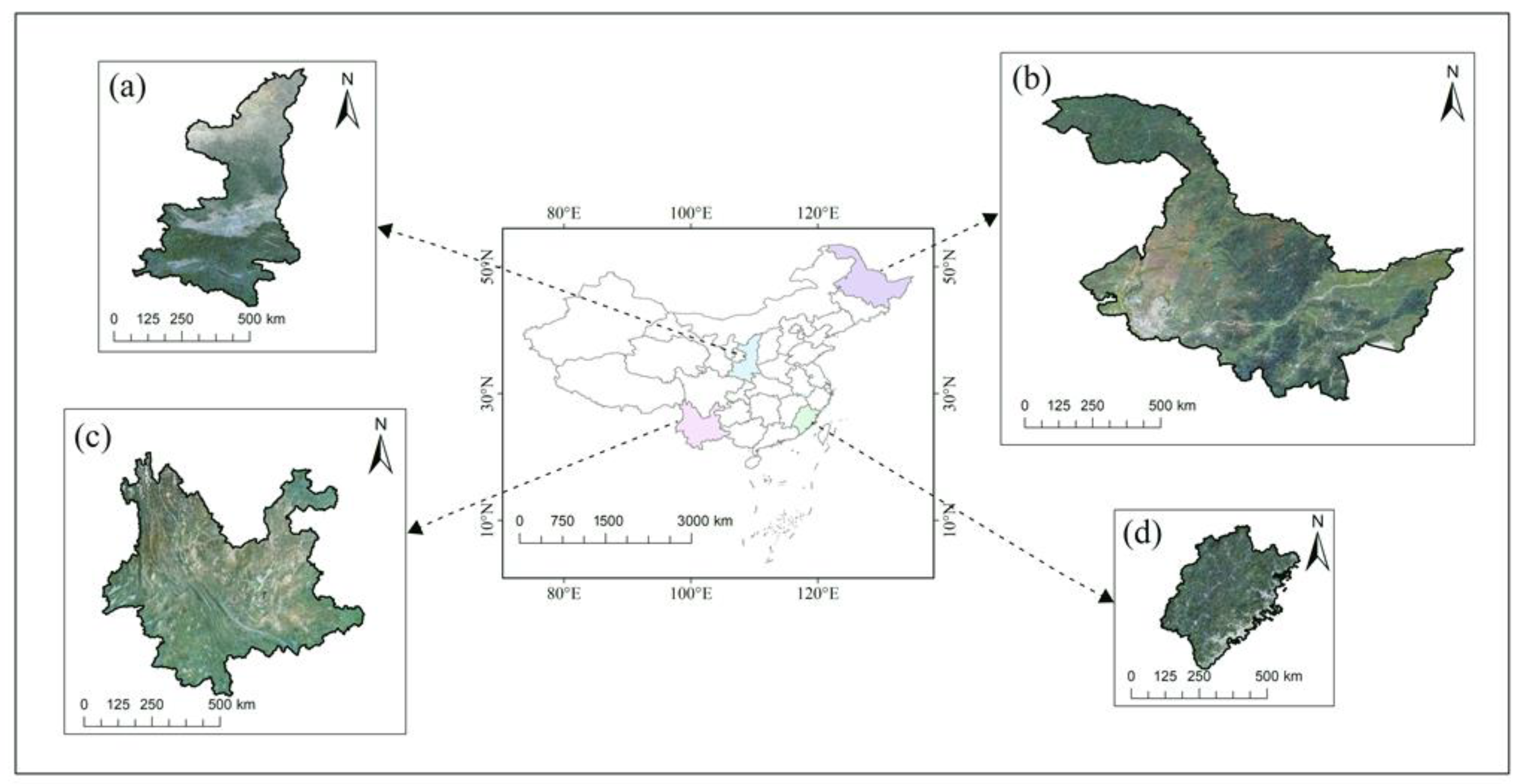
Figure 1. Spatial patterns of the study area. (a) Shaanxi province; (b) Heilongjiang province; (c) Yunnan province; and (d) Fujian province. Remote sensing images of the four provinces came from the Landsat 8 OLI data.
Remotesensing 15 00879 g001
Figure 2. Inter-annual variation and Mann–Kendall test curves of SPEI in four provinces from 2006 to 2018. UF was obtained from the forward sequence data of SPEI. UB was obtained from the inverse sequence data of SPEI. (a) Yunnan province; (b) Fujian province; (c) Shaanxi province; and (d) Heilongjiang province.
Remotesensing 15 00879 g002
Figure 3. Variation trends of SIF, SIFyield, NDVI, EVI, LAI, and fPAR standardized anomalies during drought periods in four provinces. (a) Yunnan province; (b) Fujian province; (c) Shaanxi province; and (d) Heilongjiang province.
Remotesensing 15 00879 g003
Figure 4. (a1a6) The seasonal cycle variation curves of present values and multi-year averages and the abnormal decrease amplitude of the present values from the average values of SIF, SIFyield, NDVI, EVI, LAI, and fPAR, respectively, in Yunnan province (b1b6). The seasonal cycle variation curves of present values and multi-year averages and the abnormal decrease amplitude of the present values from the average values of SIF, SIFyield, NDVI, EVI, LAI, and fPAR, respectively, in Fujian province.
Remotesensing 15 00879 g004
Figure 5. (a1a6) The seasonal cycle variation curves of present values and multi-year averages and the abnormal decrease amplitude of the present values from the average values of SIF, SIFyield, NDVI, EVI, LAI, and fPAR, respectively, in Shaanxi province (b1b6). The seasonal cycle variation curves of present values and multi-year averages and the abnormal decrease amplitude of the present values from the average values of SIF, SIFyield, NDVI, EVI, LAI, and fPAR, respectively, in Heilongjiang province.
Remotesensing 15 00879 g005
Figure 6. (a1a6) The spatial distribution of standardized anomalies of SIF, SIFyield, NDVI, EVI, LAI, and fPAR in the early drought period in Yunnan province, respectively; (b1b6) The spatial distribution of standardized anomalies of SIF, SIFyield, NDVI, EVI, LAI, fPAR in the middle drought period in Yunnan province, respectively; (c1c6) The spatial distribution of standardized anomalies of SIF, SIFyield, NDVI, EVI, LAI, fPAR in the late drought period in Yunnan province, respectively; (d1d6) The spatial distribution of standardized anomalies of SIF, SIFyield, NDVI, EVI, LAI, fPAR in the early drought period in Fujian province, respectively; (e1e6) The spatial distribution of standardized anomalies of SIF, SIFyield, NDVI, EVI, LAI, fPAR in the middle drought period in Fujian province, respectively; (f1f6) The spatial distribution of standardized anomalies of SIF, SIFyield, NDVI, EVI, LAI, fPAR in the late drought period in Fujian province, respectively.
Remotesensing 15 00879 g006
Figure 7. (a1a6) The spatial distribution of standardized anomalies of SIF, SIFyield, NDVI, EVI, LAI, fPAR in the early drought period in Shaanxi province, respectively (b1b6). The spatial distribution of standardized anomalies of SIF, SIFyield, NDVI, EVI, LAI, and fPAR in the middle drought period in Shaanxi province, respectively (c1c6). The spatial distribution of standardized anomalies of SIF, SIFyield, NDVI, EVI, LAI, and fPAR in the late drought period in Shaanxi province, respectively (d1d6). The spatial distribution of standardized anomalies of SIF, SIFyield, NDVI, EVI, LAI, and fPAR in the early drought period in Heilongjiang province, respectively (e1e6). The spatial distribution of standardized anomalies of SIF, SIFyield, NDVI, EVI, LAI, and fPAR in the middle drought period in Heilongjiang province, respectively (f1f6). The spatial distribution of standardized anomalies of SIF, SIFyield, NDVI, EVI, LAI, and fPAR in the late drought period in Heilongjiang province, respectively.
Remotesensing 15 00879 g007
Figure 8. Correlation between standardized anomalies of SIF, SIFyield, NDVI, EVI, LAI, and fPAR with SPEI. (a) Yunnan province; (b) Fujian province; (c) Shaanxi province; and (d) Heilongjiang province.
Remotesensing 15 00879 g008
Figure 9. Variable importance (x axis value) of remote sensing variables for explaining the performances of each variable in detecting drought event. (a) Yunnan province; (b) Fujian province; (c) Shaanxi province; and (d) Heilongjiang province.
Remotesensing 15 00879 g009
Table 1. Datasets used in the study.
The Data TypeProductsTimeNative Spatial ResolutionFinal Spatial ResolutionTemporal Resolution
SPEISPEIbase V2.62006–20180.5°0.05°1 month
SIFGOSIF2006–20180.05°0.05°1 month
VIsMCD43C42006–20180.05°0.05°16 d
LAIMOD15A2H2006–2018500 m0.05°8 d
fPARMOD15A2H2006–2018500 m0.05°8 d
SSRDERA5-Land2006–20180.1°0.05°1 month
Landcover dataMCD12C120120.05°0.05°year
Table 2. SPEI drought grade classification table.
GradeThe Degree of DroughtSPEI
1Non-drought−0.5 < SPEI
2Light drought−1.0 < SPEI ≤ −0.5
3Medium drought−1.5 < SPEI ≤ −1.0
4Severe drought−2.0 < SPEI ≤ −1.5
5Extreme droughtSPEI ≤ −2.0
Table 3. SIF, SIFyield, NDVI, EVI, LAI, and fPAR correctly indicated the proportion of drought area in the early/middle/late drought period in four provinces.
ProvincesDrought PeriodPercentage of Detected Drought Areas That Coincident with SPEI Drought Regions (%)
SIFSIFyieldNDVIEVILAIfPAR
Yunnanearly68.7882.3054.1453.2745.6433.96
middle73.4684.2197.2598.0451.9956.14
late38.6421.8836.1236.0523.5318.78
Fujianearly051.331.746.2211.6010.84
middle5.6171.4910.0825.1740.7129.57
late16.9127.524.7714.4025.4324.11
Shaanxiearly70.9986.0774.8366.1622.6014.81
middle46.9755.8149.7134.9841.1336.44
late44.6747.2345.0440.3817.5115.83
Heilongjiangearly73.9674.9573.6262.0943.0736.21
middle70.7974.0760.1657.3363.0130.68
late79.4780.3970.1073.2169.2258.73
Disclaimer/Publisher’s Note: The statements, opinions and data contained in all publications are solely those of the individual author(s) and contributor(s) and not of MDPI and/or the editor(s). MDPI and/or the editor(s) disclaim responsibility for any injury to people or property resulting from any ideas, methods, instructions or products referred to in the content.