Article

Automatic Modulation Recognition of Radiation Source Signals Based on Data Rearrangement and the 2D FFT

1
Science and Technology on Electromechanical Dynamic Control Laboratory, Beijing Institute of Technology, Beijing 100081, China
2
Tangshan Research Institute, Beijing Institute of Technology, Beijing 100081, China
*
Author to whom correspondence should be addressed.
Remote Sens. 2023, 15(2), 518; https://doi.org/10.3390/rs15020518
Submission received: 13 December 2022 / Revised: 9 January 2023 / Accepted: 10 January 2023 / Published: 15 January 2023

Abstract

:
It is a challenge for automatic modulation recognition (AMR) methods for radiation source signals to work in environments with low signal-to-noise ratios (SNRs). This paper proposes a modulation feature extraction method based on data rearrangement and the 2D fast Fourier transform (FFT) (DR2D), and a DenseNet feature extraction network with early fusion is constructed to recognize the extracted modulation features. First, the input signal is preprocessed by DR2D to obtain three types of joint frequency feature bins with multiple time scales. Second, the feature fusion operation is performed on the inputs of the different layers of the proposed network. Finally, feature recognition is completed in the subsequent layers. The theoretical analysis and simulation results show that DR2D is a fast and robust preprocessing method for extracting the features of modulated radiation source signals with less computational complexity. The proposed DenseNet feature extraction network with early fusion can identify the extracted modulation features with less spatial complexity than other types of convolutional neural networks (CNNs) and performs well in low-SNR environments.

1. Introduction

Automatic modulation recognition (AMR) is a process for automatically identifying the modulation type of a received signal without prior knowledge of the radiation source system [1,2]. AMR is widely used in civil and military applications and plays an important role in cognitive radio techniques that work in various cooperative and non-cooperative contexts, such as signal confirmation, interference identification, and spectrum sensing [3,4,5]. In fact, the modulation types of radiation source signals are complex and variable, and they have gradually changed from a single continuous wave type to complex modulation types such as multi-waveform frequency, pulse amplitude, and binary-code phase modulations. Moreover, the radiation source signals are often in electromagnetic environments with low signal-to-noise ratios (SNRs), reducing the identification and analysis capabilities of cognitive radio systems. It is important to correctly recognize radiation source signals with low SNRs in a short period to make appropriate decisions [6,7].
AMR can be broadly classified into three categories: likelihood-based AMR (LB-AMR) [8], distribution test-based AMR (DB-AMR) [9], and feature-based AMR (FB-AMR) [10]. FB-AMR extracts feature from modulated signals and then completes the recognition process by using a certain classifier. Many studies have been carried out on FB-AMR in recent years, most of which have employed time-frequency analysis and machine-learning methods. Reference [11] proposed a method for radar emitter recognition based on a scale-invariant feature transform (SIFT) position and scale features by performing a short-time Fourier transform (STFT) on the radar emitter signal, extracting SIFT scale and position features from the time-frequency image, and using a support vector machine (SVM) for automatic recognition. Reference [12] proposed a low intercept probability (LPI) radar waveform recognition method based on a dual-channel convolutional neural network (CNN) and feature fusion by converting LPI radar waveforms into two-dimensional time-frequency images through the Choi–Williams distribution (CWD), extracting a directional histogram of oriented gradient (HOG) features, and depth features from the time-frequency images through the dual-channel CNN and using a multilayer perceptron (MLP) network to fuse these features and distinguish the types of LPI radar signals. Reference [13] used the Fourier-based synchrosqueezing transform (FSST) as a means of data augmentation and transformation, demonstrating that a CNN can better learn time-frequency image features from the FSST than from the STFT. Reference [14] demonstrated that in radar-communication coexistence and shared-spectrum scenarios, a CNN model with the FSST time-frequency analysis method has good waveform classification performance. Reference [15] addressed the problem of automatic waveform recognition in coexistence radar-communication systems by using a smooth pseudo-Wigner–Ville distribution (SPWVD) for time-frequency analysis, and proposed an efficient CNN with several processing blocks that integrate residual connections and attention connections. The average recognition accuracy was approximately 17.6% higher than that of a fuzzy SVM recognition model.
The AMR methods described above obtain modulation characteristics mainly by generating time-frequency images. Time-frequency energy aggregation methods can retain clear and sufficient features for recognition in low-SNR environments but have large computational complexity levels. A feature recognition model using a machine learning method cannot be effectively adapted to the time-frequency image feature analysis situation, resulting in unnecessary floating-point computations and model parameters. Aiming at the above problems, this paper proposes a feature extraction method based on data rearrangement and the 2D fast Fourier transform (FFT) (DR2D) to obtain the joint frequency features of the input modulated signal at multiple time scales and constructs a DenseNet feature extraction network with early fusion to recognize the joint frequency features of the rearranged signal. The theoretical analysis and simulation results show that the proposed network combined with the DR2D preprocessing method can quickly recognize the modulation types of radiation source signals and achieve good recognition accuracy in low-SNR environments.

2. Feature Extraction Method Based on Data Rearrangement and the 2D FFT

2.1. Data Rearrangement

In linear frequency modulation continuous wave (LFMCW) radar, the echo pulses of different distance units are rearranged into a two-dimensional matrix, while the distance and velocity of the target are determined by the 2D FFT operation [16]. Synthetic aperture radar (SAR) achieves dual localization of the target in terms of distance and orientation by segmenting and storing the echoes of different pulse intervals in the form of a two-dimensional array and also performing a 2D FFT operation [17]. All these methods essentially segment one-dimensional signals at slow and fast time scales, rearrange them into corresponding two-dimensional data and realize the dual confirmation of frequency features at the two time scales via the 2D FFT operation. Theoretically, the joint frequency characteristics of an unknown radiation source signal can be obtained by rearranging one-dimensional data into multidimensional arrays with multiple time scales and using a multidimensional FFT algorithm.
The process of the modulation feature extraction method based on DR2D is shown in Figure 1. First, the received signal is segmented at the slow time scale, and then the fragments with the slow time scales are further segmented at two different time scales: inferior-fast and fast time scales. Second, the signal segments with the inferior-fast and fast time scales are rearranged into two-dimensional matrices, called data slices, and stacked at a slow time scale into a rearranged data bin. Finally, the joint frequency feature slices are obtained by performing 2D FFT operations on the different data slices and are further rearranged into a joint frequency feature bin by performing stacking on the slow time scale.

2.2. Two-Dimensional FFT

We assume that the i th data slice of the input signal is an M × M matrix X i , on which a 2D FFT operation is performed to obtain the i th spectral matrix and the corresponding joint frequency feature slice as follows:
Y i ( m , n ) = k = 0 M 1 l = 0 M 1 X i ( k , l ) e j 2 π M k m e j 2 π M l n
Y i ( m , n ) = Y i ( m , n ) y min y max y min
where the modulo numbers of the spectral matrix, Y i , are normalized as the joint frequency feature slice Y i , y max and y min are the maximum and minimum values in Y i , and m , n = 0 , 1 , · · · , M 1 , which means that X i and Y i will have the same sizes and dimensions.
Y i can be seen either as a magnitude spectrum of two-dimensional data in the frequency domain or a grayscale image reflecting the changing patterns of the signal. In contrast to performing a 1D FFT on the real signal, which gives a spectrum that is symmetrically distributed about the zero frequency point, implementing a 2D FFT on the data slices gives a joint frequency feature slice that is centrosymmetrically distributed about the center point.
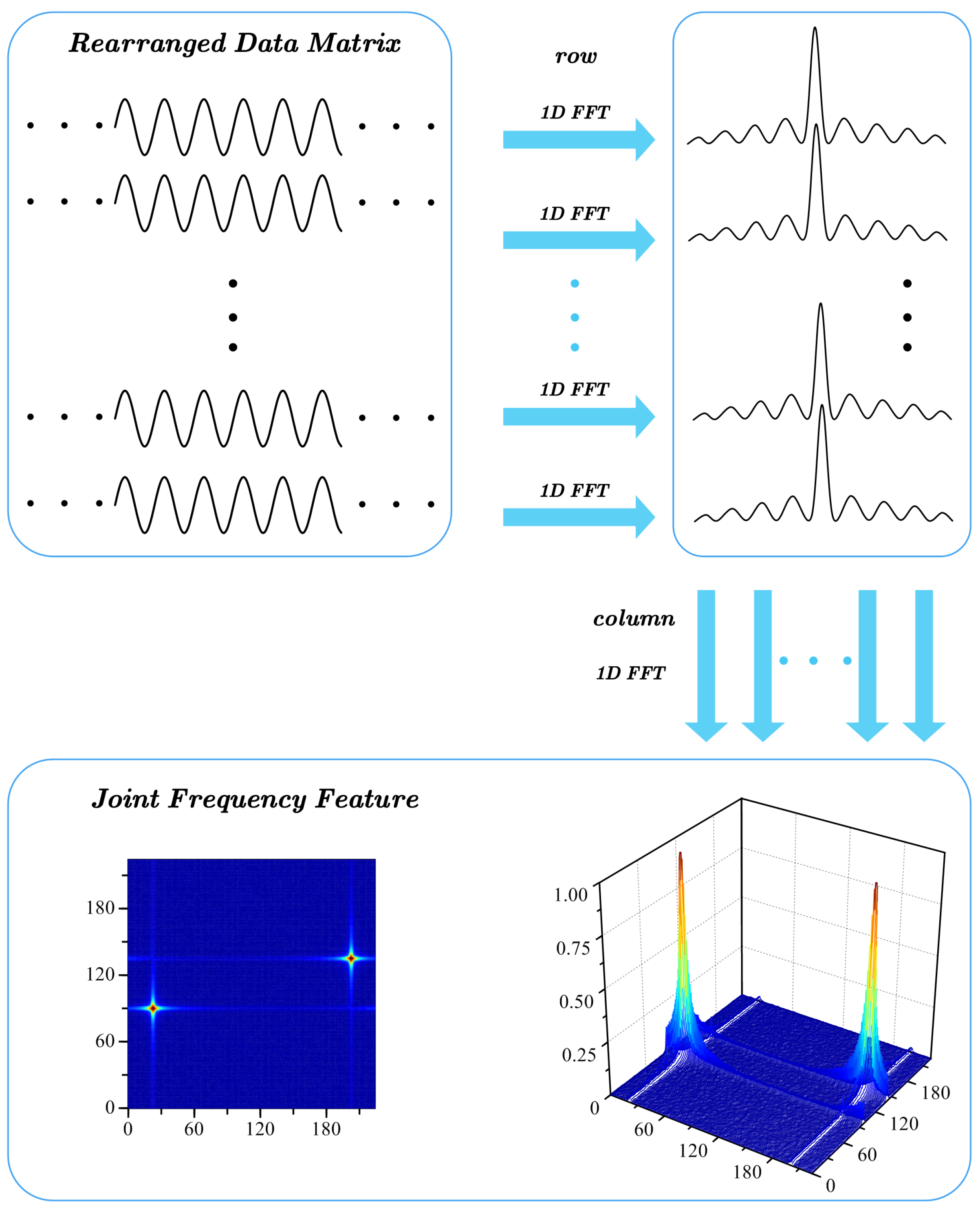
From the perspective of signal analysis, performing a 2D FFT operation on the data slice is equivalent to performing a 1D FFT operation on each row of the data matrix (i.e., data points on the fast time scale), and then performing a 1D FFT operation on each column of the data matrix (i.e., data points on the inferior-fast time scale), as shown in Figure 2. The former can effectively reflect the carrier frequency characteristic of the signal, while the latter can better reflect the frequency bias characteristic of the signal, and the variation exhibited by the feature slices at a slow time scale can reflect the modulation pattern of the signal. The smaller the data slices are, the denser the segmentation at the slow time scale, while the frequency variation of the signal will be reflected in more detail. If N data slices are segmented at a slow time scale with no overlap, the result is called an N-level dense rearrangement pattern (DRP). If the number of overlap points is 1/K for each data slice, this result is called an N/K-level DRP. The different joint frequency feature slices represent the local features of the signal at different periods.
From the perspective of image processing, the normalized data slice can be regarded as an image with a certain texture feature, as shown in Figure 3. The 2D FFT operation implemented on the image reflects the composition of the plane wave of each frequency component in the original image. The center point of the feature image corresponds to the zero frequency, the part near the center point corresponds to the low-frequency components, and the part far from the center corresponds to the high-frequency component. The frequency level reflects the change pattern of the original grayscale image. The larger the data slice is, the more the data points will be aggregated, and the more distinct the texture features are. If the slow time scale overlaps with the inferior-fast time scale, the signal is rearranged into one data slice as a whole, and the 2D FFT reflects the global feature, which is called the overall rearrangement pattern (ORP) of the signal.

2.3. Feature Feasibility Analysis

Time-frequency analysis is often used to extract the joint time-frequency characteristics of modulated radiation source signals in AMR, such as STFT and a Wigner–Ville distribution (WVD). The longer the time window of the STFT is, the worse the time resolution and the better the frequency resolution that can be shown. At the same time, this also makes the frequency energy scattered throughout the window length, which is not conducive to feature discrimination. The synchrosqueezing transform (SST) can effectively concentrate the original dispersion of the time-frequency distribution in the time-frequency component where the useful features are located [18,19]. The WVD algorithm has better time-frequency resolution, but due to the bilinear nature of the transform, there are cross terms in the distribution of the sum of different signal components. The SPWVD algorithm retains the good time-frequency aggregation characteristic of the WVD, while greatly suppressing the generation of cross terms, allowing for better discrimination of time-frequency characteristics in low-SNR environments [20,21].
The 2D FFT is linearly weighted like the 1D FFT, and there are no cross terms between different signal components. The frequency features extracted by DR2D are more aggregated in terms of energy because of the intersection of the smearing of energy distribution at horizontal and vertical frequency components, resulting in a strong fixed frequency characteristic. Thus, even with a small-sized data slice, the frequency resolution is still good in low-SNR environments, and the signal components that overlap in the frequency domain can also be effectively separated.
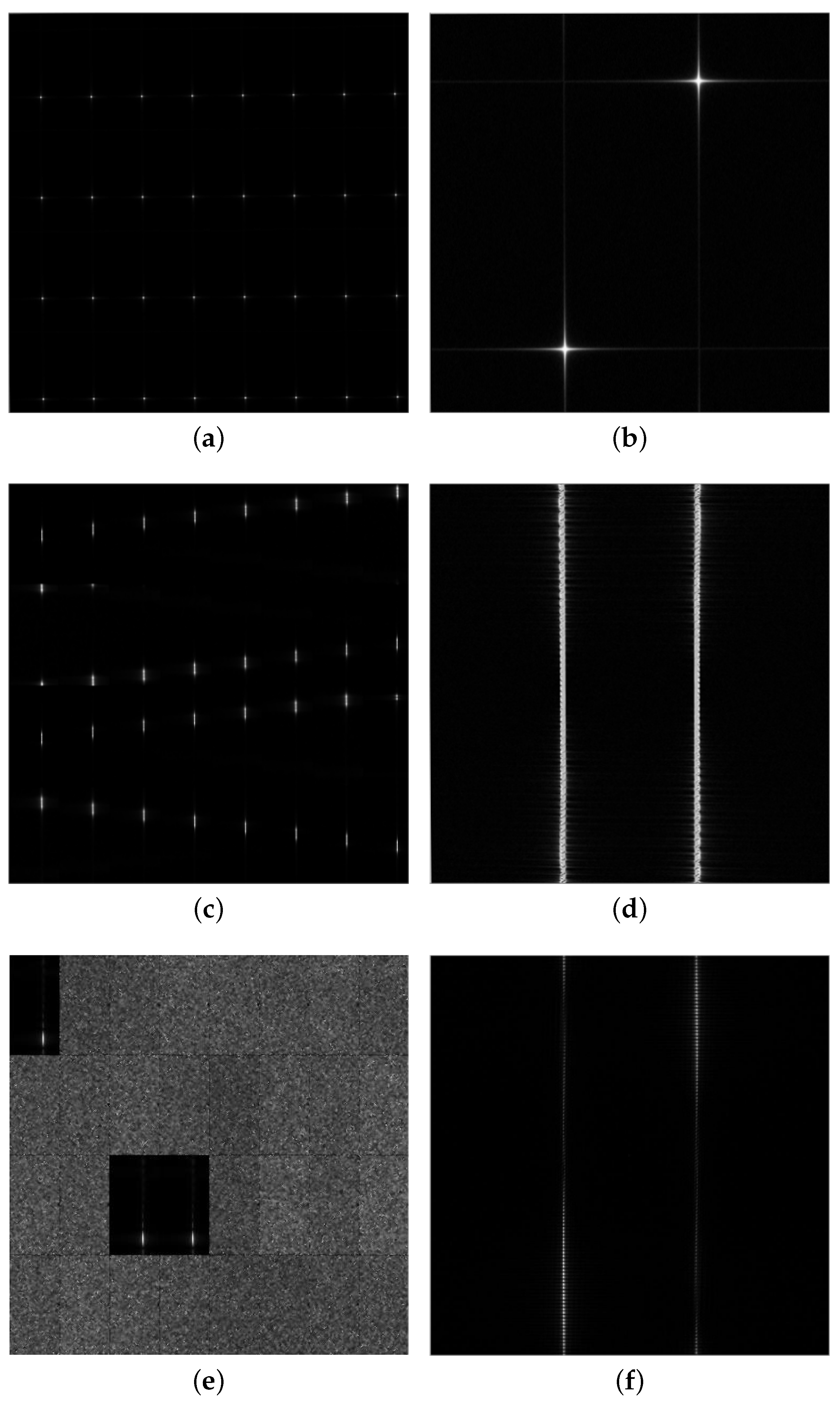
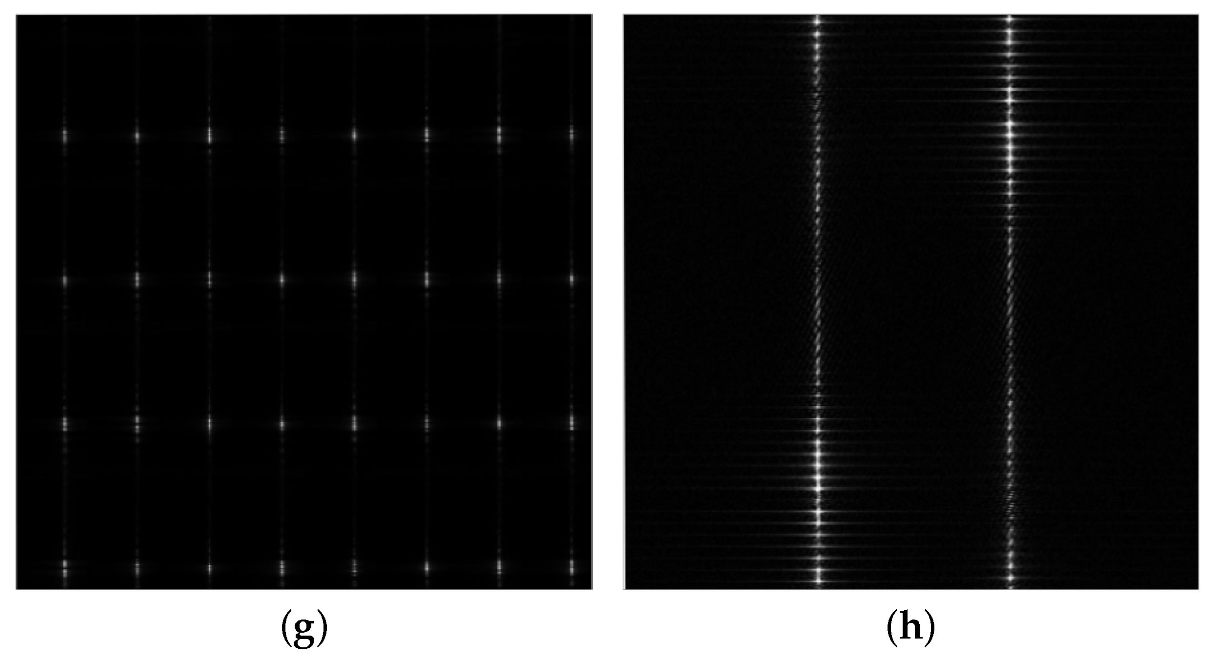
Due to the centrosymmetry of the spectrum obtained by the 2D FFT, the joint frequency feature slices obtained by DR2D can be cut in half and concatenated to easily observe the local features of the signal. Four typical modulation types of radiation source signals are selected for the analysis: the carrier frequency of the continuous wave signal and the other three types of radiation source signals, all at 5 GHz; a triangle wave frequency modulation signal modulated at a frequency of 100 kHz with a bandwidth of 400 MHz; a pulse amplitude modulation signal with a pulse width of 50 ns and a duty cycle of 1%; and a binary phase shift keying signal with a code element width of 50 ns. Please see Appendix A for the models of the modulation signals. The four radiation source signals are under 32/2-level DRPs and ORPs in the SNR environment of 20 dB, with the joint frequency features shown in Figure 4. It can be seen that the continuous wave signal shows a cross-shape joint frequency feature in both patterns, with the frequency components concentrated at the center of the cross; it has a strong fixed frequency characteristic. The triangle wave frequency modulation signal produces a linear shift in the joint frequency feature, with the frequency components broadening on the inferior-fast time scale under the DRP; it exhibits a regular pinstripe with the frequency components extending to the entire inferior-fast time scale under the ORP, reflecting the modulation pattern and bandwidth characteristic of the signal. The pulse amplitude modulation signal only shows the specific frequency characteristics in the data slices where the pulse exists under the DRP, while it shows a regular dotted line under the ORP. The binary phase shift keying signal shows an irregularly spreading shape in both patterns.
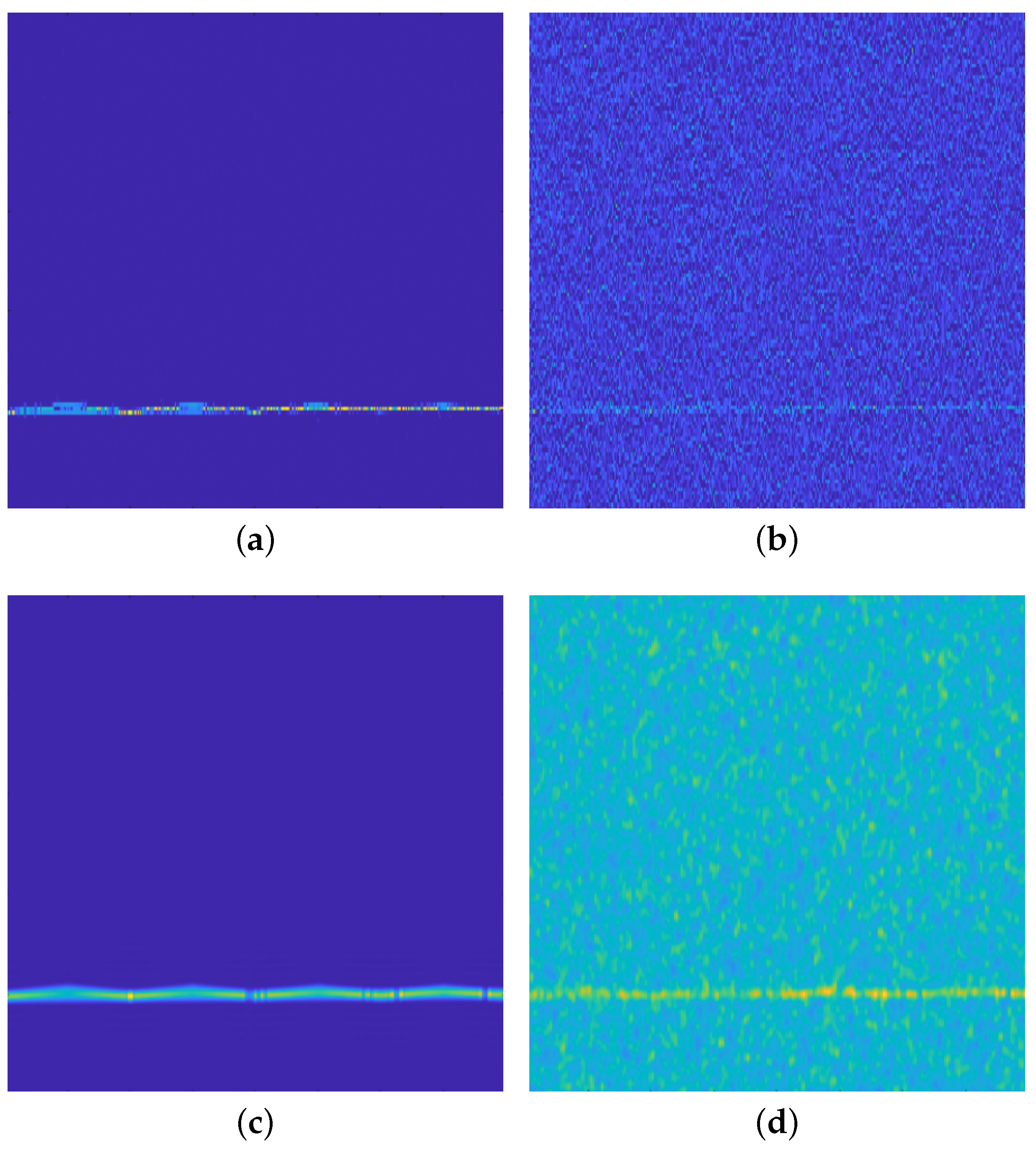
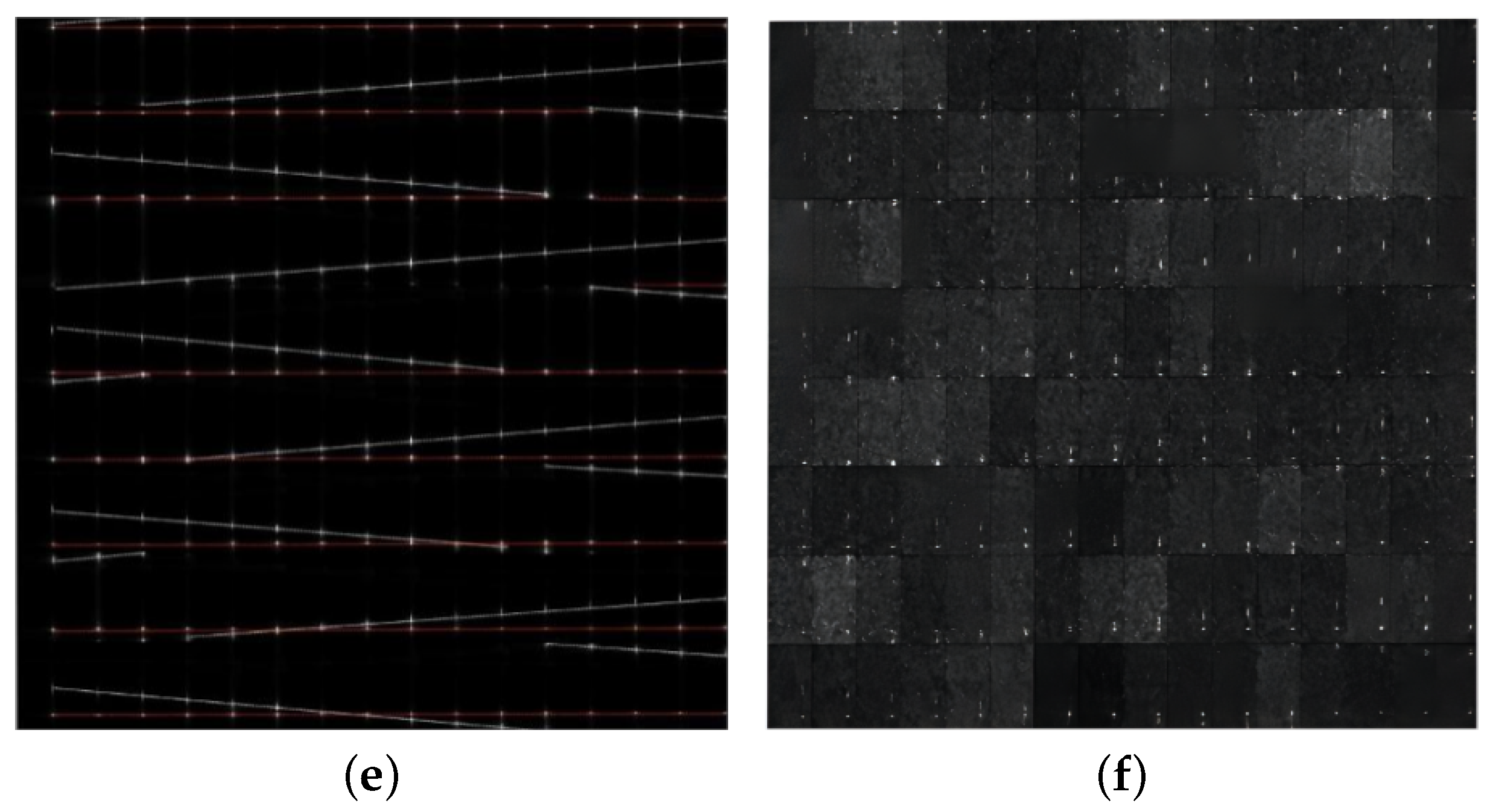
For two different triangle wave frequency modulation signals with overlap in the frequency domain, the carrier frequencies are 5 GHz and 5.1 GHz, the modulation frequencies are 100 kHz and 1 MHz, and the modulation bandwidths are 400 MHz and 600 MHz. In SNR environments of 20 dB and −15 dB, the joint frequency features under a 128/2-level DRP and the time-frequency images obtained by the FSST and SPWVD are shown in Figure 5 (the red line and the white line represent the modulation patterns of the two signals, respectively). It can be seen that neither the FSST nor the SPWVD is able to discriminate the multicomponent signals with overlap in the frequency domain, while the feature extraction method based on DR2D can better reflect the details of the modulation pattern under the DRP with good noise immunity and high resolution for signals with different parameters that overlap in the frequency domain, even in a low-SNR environment.
The relative bandwidth of the signal affects the visualization range of the useful frequency components on the feature image. The greater the relative bandwidth, the larger the visualization range. The modulation bandwidth of the radiation source signal is f B W , and the carrier frequency is f c ; thus, the relative bandwidth can be expressed as follows:
f f o c = f B W f c
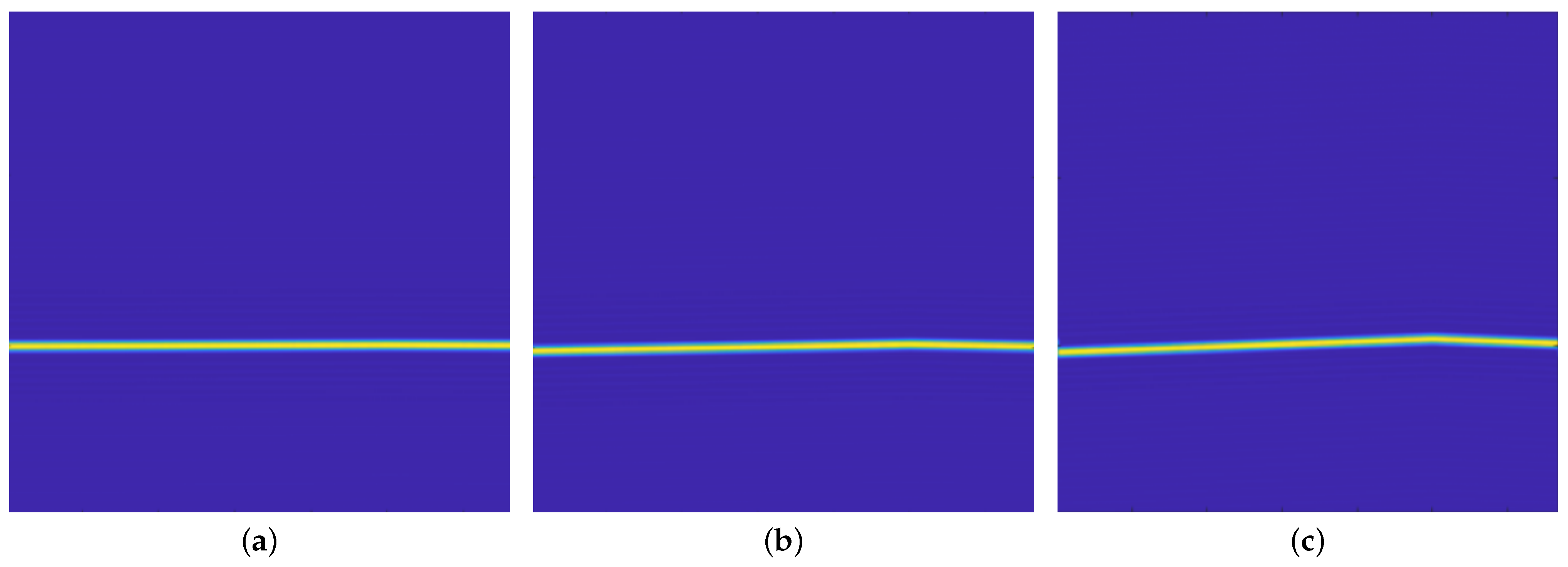
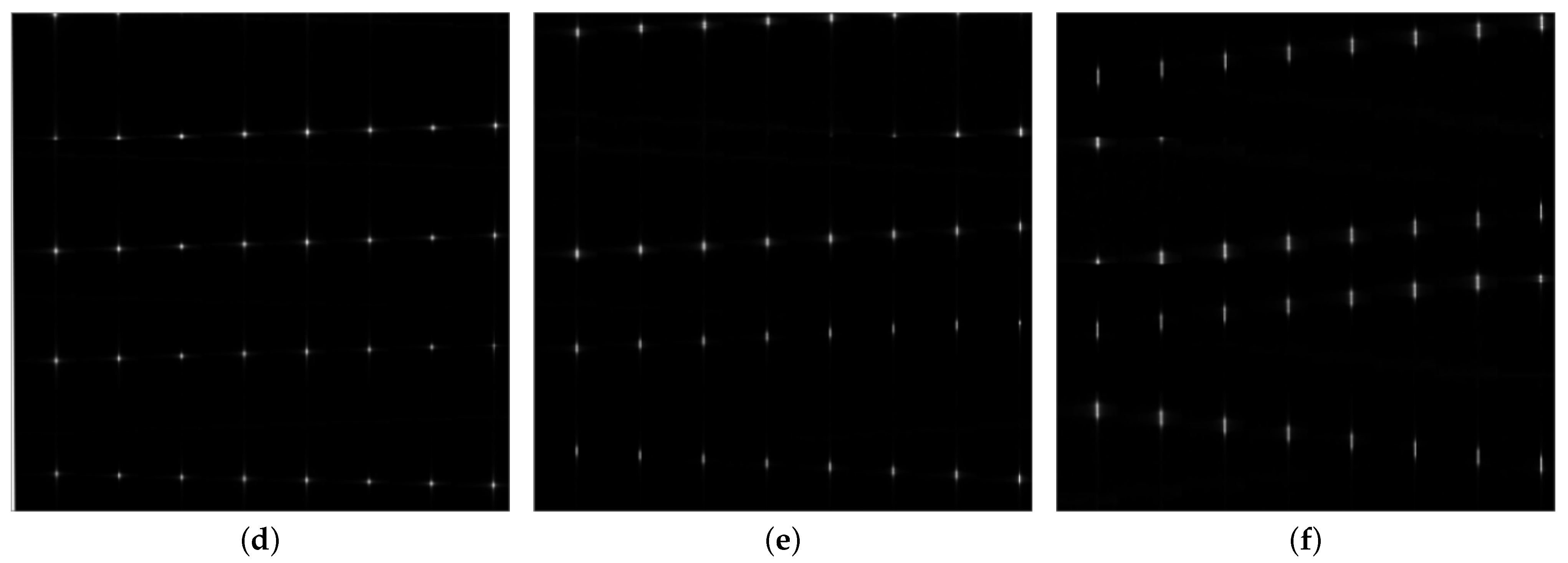
For triangle wave frequency modulation signals with the same frequency modulation slope and different relative bandwidths, the feature images obtained by DR2D and the SPWVD are shown in Figure 6. It can be seen that the discernibility of frequency changes in the time-frequency image is very much limited by the relative bandwidth, and the joint frequency feature of DR2D shows a cyclic pattern of changes in the vertical direction, with the changes being displayed from the opposite end when they exceed the size of the slice. On the one hand, the DR2D feature images are disconnected at a certain point under continuously varying frequencies. On the other hand, this cyclic pattern results in better discernibility and a better visualization range for the useful frequency components, which is advantageous for modulation recognition with a low relative bandwidth.

3. Feature Recognition Via the DenseNet Feature Extraction Network with Early Fusion

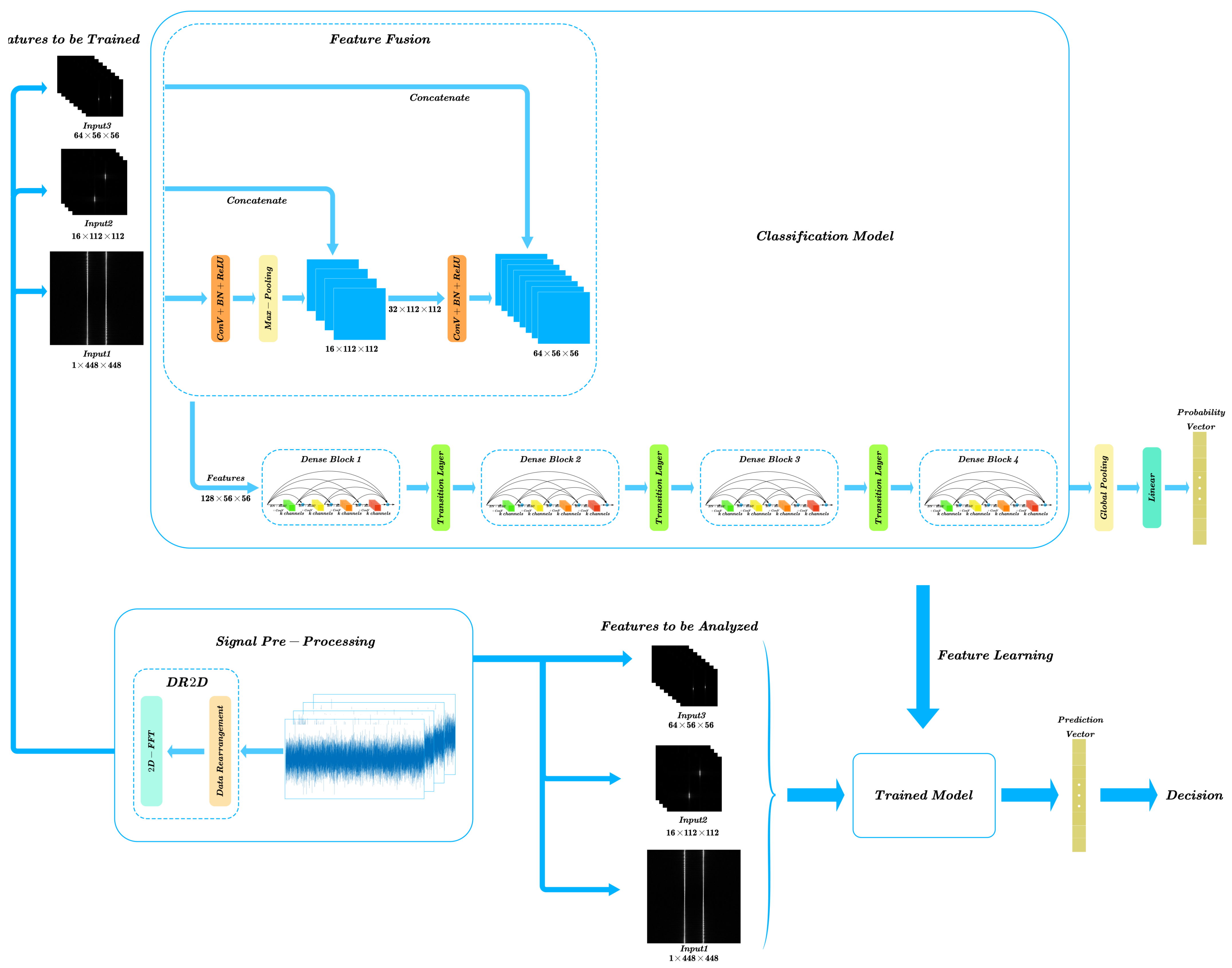
A schematic diagram of the feature recognition process using the DenseNet feature extraction network with early fusion is shown in Figure 7. The radiation source signal was segmented and rearranged under three different rearrangement patterns, and the feature slices obtained by 2D FFT processing were fed into different layers of the network as input grayscale feature maps and concatenated for model training and classification. Consequently, the modulation type of the radiation source signal was recognized by the trained model.

3.1. Signal Preprocessing

The data slices were considered texture images for analysis and needed to be normalized; i.e., the original signal values were mapped to pixel values in the range of 0∼1, which is equivalent to the superimposition of a DC component after imposing an overall enlargement or reduction on the original signal. Therefore, the zero-frequency maxima in the center of the feature slice image should first be removed after the 2D FFT operation and before normalization.
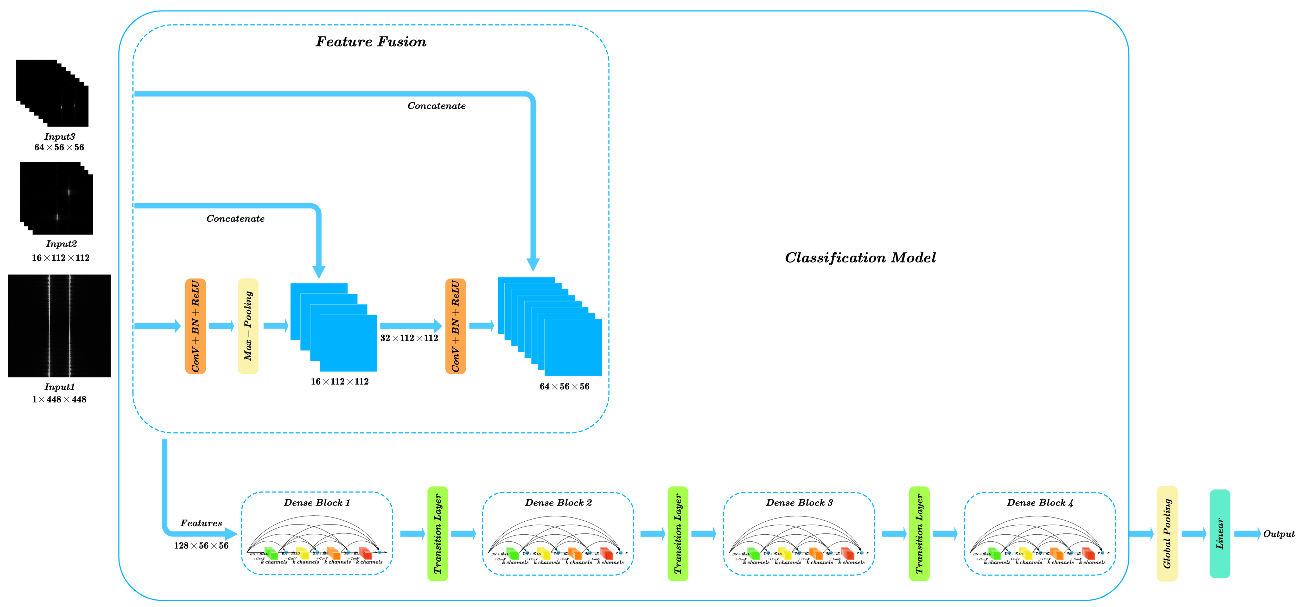
To fully extract the modulation features, the DR2D preprocessing method was performed on the radiation source signal under three rearrangement patterns, which are shown in Figure 8. With 448 × 448 points in length, a 64 × 56 × 56 joint frequency feature bin was obtained by a 64-level DRP, reflecting the frequency variation features in detail; a 16 × 112 × 112 joint frequency feature bin was obtained by a 32-level DRP, which also reflects changes of the joint frequency features with more aggregation in case of overly dense segmentation by the 64-level DRP; and a 1 × 448 × 448 joint frequency feature bin was obtained under the ORP to reflect the texture feature of the signal as a whole. Three joint frequency feature bins needed 64 × 2 × 56 56-point FFTs, 16 × 2 × 112 112-point FFTs and 1 × 2 × 448 448-point FFTs, respectively. The obtained feature bins were used as the grayscale input feature maps of different layers of the network, and the feature fusion operation was completed in those layers as well. On the one hand, we choose 448 × 448 points to fully reflect the modulation feature of the radiation source signal with high frequency. On the other hand, the feature maps obtained from the three rearrangement patterns can be concatenated at the same size after performing convolution and pooling operations.

3.2. DenseNet Feature Extraction Network with Early Fusion

ResNet allows a deeper network to be easily trained and optimized by introducing a residual learning framework, which can effectively alleviate the problems of vanishing gradients, exploding gradients, and network degradation caused by network deepening [22]. DenseNet directly reuses features by establishing dense connections between all previous layers and the current layer, which naturally integrates the properties of identity mappings and deeply strengthens the informational flow, resulting in higher performance with substantially fewer parameters and computations than those required by ResNet [23,24].
The basic modules of DenseNet include dense blocks and transition layers.

3.2.1. Dense Block

In the dense block, the feature maps output from all previous layers are concatenated and used as inputs of the current layer to achieve dense connections between the layers. Assuming that a nonlinear transformation function can be fitted between the input and the output of a layer, the th-layer nonlinear transformation functions H · of the conventional CNN, ResNet, and DenseNet are:
x = H x 1
x = H x 1 + x 1
x = H [ x 0 , x 1 , . . . , x 1 ]
where x and x 0 , x 1 , . . . , x 1 represent the outputs of the th layer and all previous layers, respectively.
Unlike the post-activation architecture in the conventional CNN and ResNet, DenseNet utilizes pre-activation architecture by applying batch normalization (BN) and a rectified linear unit (ReLU) activation function, before performing convolution (Conv) rather than after. This minor change yields better performance.
Assuming that k 0 input feature maps are placed into a dense block and each layer has k output channels, then the th layer has k 0 + k · ( l 1 ) input feature maps, where k is called the growth rate of the network. A 4-layer dense block is shown in Figure 9.

3.2.2. Transition Layer

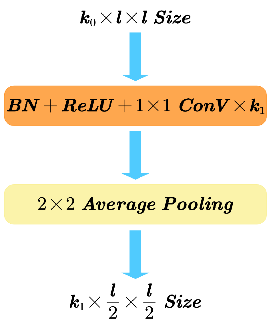
The purpose of the transition layer was to connect adjacent dense blocks by adjusting the number and sizes of feature maps. The transition layer shown in Figure 10 consists of two main parts, convolution and average pooling. The 1 × 1 convolutional layer after the BN operation and the ReLU function was used to adjust the number of feature maps and prevent the network depth from drastically increasing due to the concatenation processes in the dense blocks. The 2 × 2 average pooling layer compressed the feature map size to 1/4 of the original size by downsampling. The convolution layer and the average pooling layer together served to reduce the dimensionality of the network.

3.2.3. Network Architecture

A DenseNet feature extraction network with early fusion was denoted as DenseNet-F. DenseNet-F22 was constructed as shown in Figure 11. The feature fusion module was used for multi-feature inputs by adjusting the input feature maps of different patterns to the same size. First, a 7 × 7 convolutional layer (stride 2) and a 3 × 3 max pooling layer (stride 2) adjusted the size of input joint frequency feature bin 1 ( 1 × 448 × 448 ) to feature maps with the same size as input joint frequency feature bin 2 ( 16 × 112 × 112 ), so that joint frequency feature bin 1 and joint frequency feature bin 2 had the same feature information weight, and 32 × 112 × 112 fused feature maps were obtained by concatenating the adjusted feature maps with joint frequency feature bin 2. Second, a 3 × 3 convolutional layer (stride 2) followed by BN and the ReLU function, adjusted the 32 × 112 × 112 fused feature maps to the same size as input joint frequency feature bin 3 ( 64 × 56 × 56 ), at which time joint frequency feature bin 3 had the largest feature information weight to reflect more detail. Finally, the same concatenation process was performed to complete the feature fusion procedure for the three joint frequency feature bins. The feature extraction module of the network consisted of four 4-layer dense blocks and three transition layers. Each dense block had a growth rate of k = 32 (which was proven to be effective in [23,24]), so that the number of feature maps output by a 4-layer dense block was still the same as the number of input feature maps, which was 128. The size of 7 × 7 output feature maps could be obtained after the adjustment performed by three transition layers for the global pooling operation. The DenseNet-F22 structure described above allowed for a stable depth and a small number of network parameters.

4. Simulation Analysis

4.1. The Simulation Environment

In this paper, the operating computer system was Windows 10, the CPU was an Intel(R) Core(TM) i7-10875H @ 2.30 GHz, the GPU was an NVIDIA GeForce RTX 2060 with Max-Q Design (6 GB), the radiation source signals were preprocessed in the MATLAB environment, and the feature recognition networks were trained and tested in the PyTorch environment.

4.2. Computational Complexity of the Preprocessing Methods

The DR2D, FSST, and SPWVD preprocessing methods were implemented separately on the received radiation source signal. The three rearrangement patterns of DR2D can be considered the 56-point, 112-point, and 448-point time windows, so a window length in the range of 56 to 448 is appropriate for conducting a time-frequency analysis. The FSST used a 256-point Hamming window in the time domain, and the SPWVD used 255-point Hamming windows in the time and the frequency domains. Considering the resolution of the time-frequency analysis, the smaller the hop size of the time domain window, the better was the time resolution, but more computations were also needed. We set the hop size to be 1/8 of the window length, which means the time domain windows all utilized 32-point hop steps in this paper, for good time resolutions and acceptable computations. We assumed that the radiation source signals had N = n × n points, and n a points were calculated in one FFT after performing zero padding. Considering the number of multiplications, the computational complexity of an n a -point FFT was O ( n a log 2 n a ) [25]. As regards to DR2D preprocessing method, 64 × n 8 × n 8 , 16 × n 4 × n 4 and 1 × n × n sizes of joint frequency feature bins could be obtained under three rearrangement patterns, needing 64 × 2 × n 8 n 8 -point FFTs, 16 × 2 × n 4 n 4 -point FFTs, and 1 × 2 × n n-point FFTs, respectively, due to the 1D FFT operations performed on each row and column. As regards to the FSST preprocessing method, there were n 2 32 n a -point FFTs, n 2 32 times of time domain windowing, and n a times of multiplications for each windowing operation. As regards to SPWVD preprocessing method, there were n 2 32 times of correlation calculations for the points in time domain windows, n 2 32 2 n a -point FFTs due to the correlation calculation, n 2 32 times of both time domain windowing and frequency domain windowing, n a times of multiplications for each windowing operation, and n a 2 times of multiplications for each correlation calculation. Please see Appendix B for the FSST and SPWVD equations. The computational complexities of the three preprocessing methods are shown in Table 1. It can be seen that the computational complexity of the DR2D preprocessing method was much lower than that of FSST and SPWVD.
We recorded each signal preprocessing time and took the average value. The average processing times were 18.30 ms for DR2D, 128.75 ms for the FSST, and 207.13 ms for the SPWVD, showing that the DR2D preprocessing method can significantly reduce the time spent on modulation feature extraction compared to that required for the time-frequency analysis process.

4.3. Network Architectures for Feature Recognition

The architectures of the 22-layer DenseNet feature extraction network with early fusion, the conventional 22-layer DenseNet, and an 18-layer ResNet [22] are shown in Table 2. It can be seen that DenseNet-F22 and DenseNet-22 have significantly fewer parameters and floating-point operations (FLOPs) than ResNet-18. DenseNet-F22 had the smallest numbers of parameters and FLOPs compared to DenseNet-22 and ResNet-18, which means that DenseNet-F22 required less spatial complexity and fewer computations.
As a GPU is limited by the memory access costs and the optimization degrees of different modules, the CPU performance could more accurately reflect the inference times achieved with the same hardware resources. We recorded each signal feature inference time and took the average value. Average inference times were 32.12 ms for DenseNet-F22, 34.32 ms for DenseNet-22, and 35.69 ms for ResNet-18 (the inference times produced by the same network for the FSST and SPWVD time-frequency images were comparable, so the average value was taken here as well). The simulation showed that the average inference time of DenseNet-F22 was shorter than those of DenseNet-22 and ResNet-18.
Taking the preprocessing and inference times into account, the DenseNet feature extraction network with early fusion combined with the DR2D preprocessing method had a faster modulation type recognition process with less resource consumption than other common CNNs combined with time-frequency analysis methods.

4.4. Recognition Accuracy

Six typical radiation source signal modulation types were selected for recognition, including continuous wave (CW) modulation, triangle wave frequency modulation (TRIFM), sine wave frequency modulation (SINFM), pulse amplitude modulation (PAM), binary phase shift keying (BPSK), and linear frequency modulation pulsing (LFM_PULSE). The DR2D, FSST, and SPWVD preprocessing methods were used to produce the corresponding datasets. In environments in the SNR range of 5 dB to −10 dB, 1000 samples were produced for each radiation source signal modulation type with the three preprocessing methods. We divided 80% of the samples into training sets and 20% into testing sets. The parameters of typical radiation source signals are listed in Table 3, where CF is the carrier frequency, MF is the modulation frequency, FD is the frequency deviation, PW is the pulse width, DC is the duty cycle, and EW is the code element width.
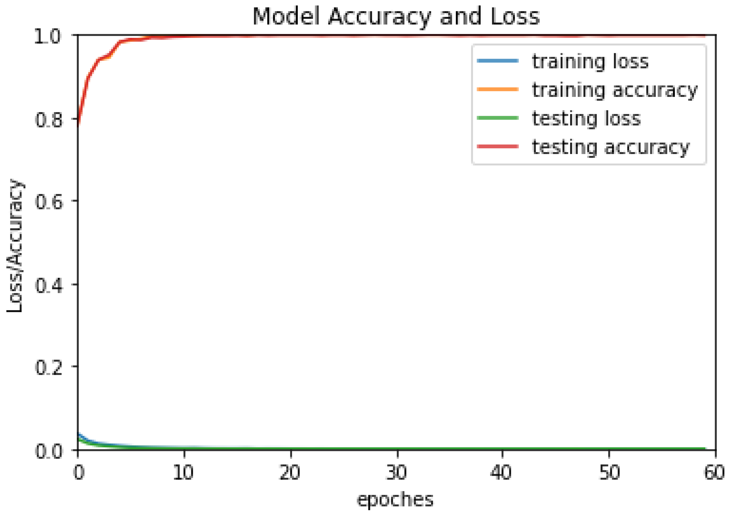
DenseNet-F22 combined with the DR2D preprocessing method was trained and tested on the dataset. The number of training epochs was set to 60, and the learning rate was set to 0.00001. The training and testing loss curves and the corresponding accuracy curves versus the number of epochs are shown in Figure 12. It can be seen that both the training set and testing set loss functions converged quickly and gradually stabilized, which means that the parameters of DenseNet-F22 were rational and that the model was effective for AMR tasks.
DenseNet-F22, DenseNet-22, and ResNet-18 combined with different preprocessing methods were trained and tested on the different datasets, and the trained models were used to recognize the six different radiation source signal modulation types in environments with SNRs ranging from 0 dB to −20 dB. Consequently, the average recognition accuracy curves obtained from the simulation are shown in Figure 13. It can be seen that both DenseNet-F22 and DenseNet-22 were able to achieve comparable or even higher accuracy than ResNet-18 with fewer model parameters under a similar number of network layers. DenseNet-22 and ResNet-18 combined with the SPWVD preprocessing method had relatively lower average recognition accuracy with SNRs lower than −12dB. DenseNet-F22 combined with the DR2D preprocessing method maintained an average recognition accuracy of more than 90% in environments with SNRs higher than −14 dB, which is comparable to that of DenseNet-22 combined with the FSST preprocessing method.
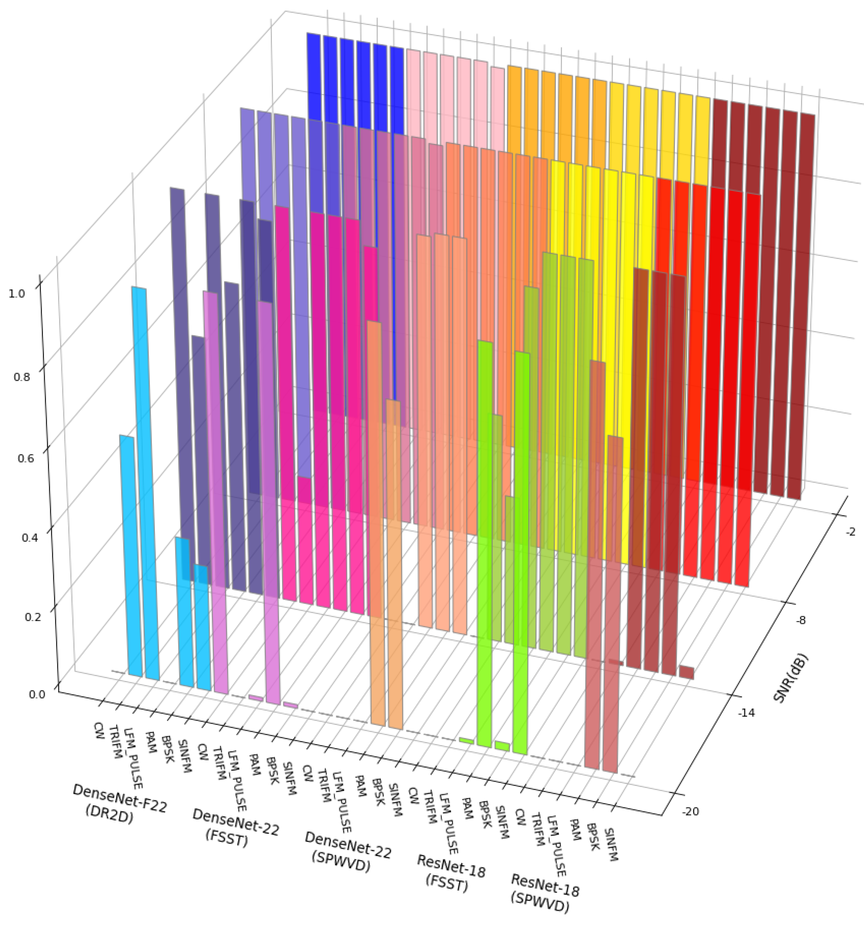
The recognition accuracy of each modulation type in environments with different SNRs is shown in Figure 14. DenseNet-22, combined with FSST was better at the recognition of CW and PAM, ResNet-18 combined with FSST was better at the recognition of PAM and SINFM, while DenseNet-22 and ResNet-18 combined with SPWVD were better at the recognition of PAM and BPSK. It can be seen that DenseNet-22 and ResNet-18 combined with FSST and SPWVD preprocessing methods had better recognition performance of certain modulation types, but worse for others, which means DenseNet-22 and ResNet-18 feature recognition networks had difficulty in avoiding the overfitting of certain modulation types, and were not conducive to the overall recognition. DenseNet-F22 combined with the DR2D preprocessing method maintained a recognition accuracy of more than 60% for each modulation type in environments with SNRs higher than −14 dB, providing the most robust recognition performance.
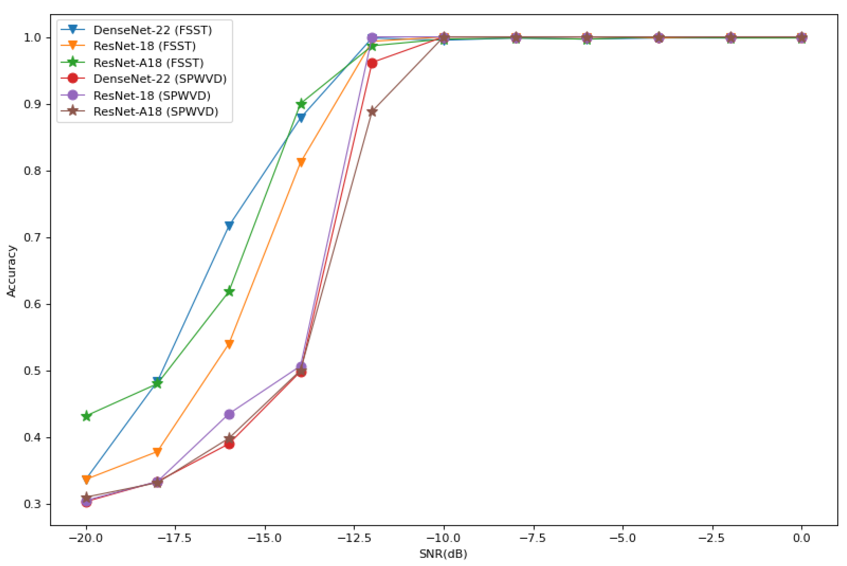
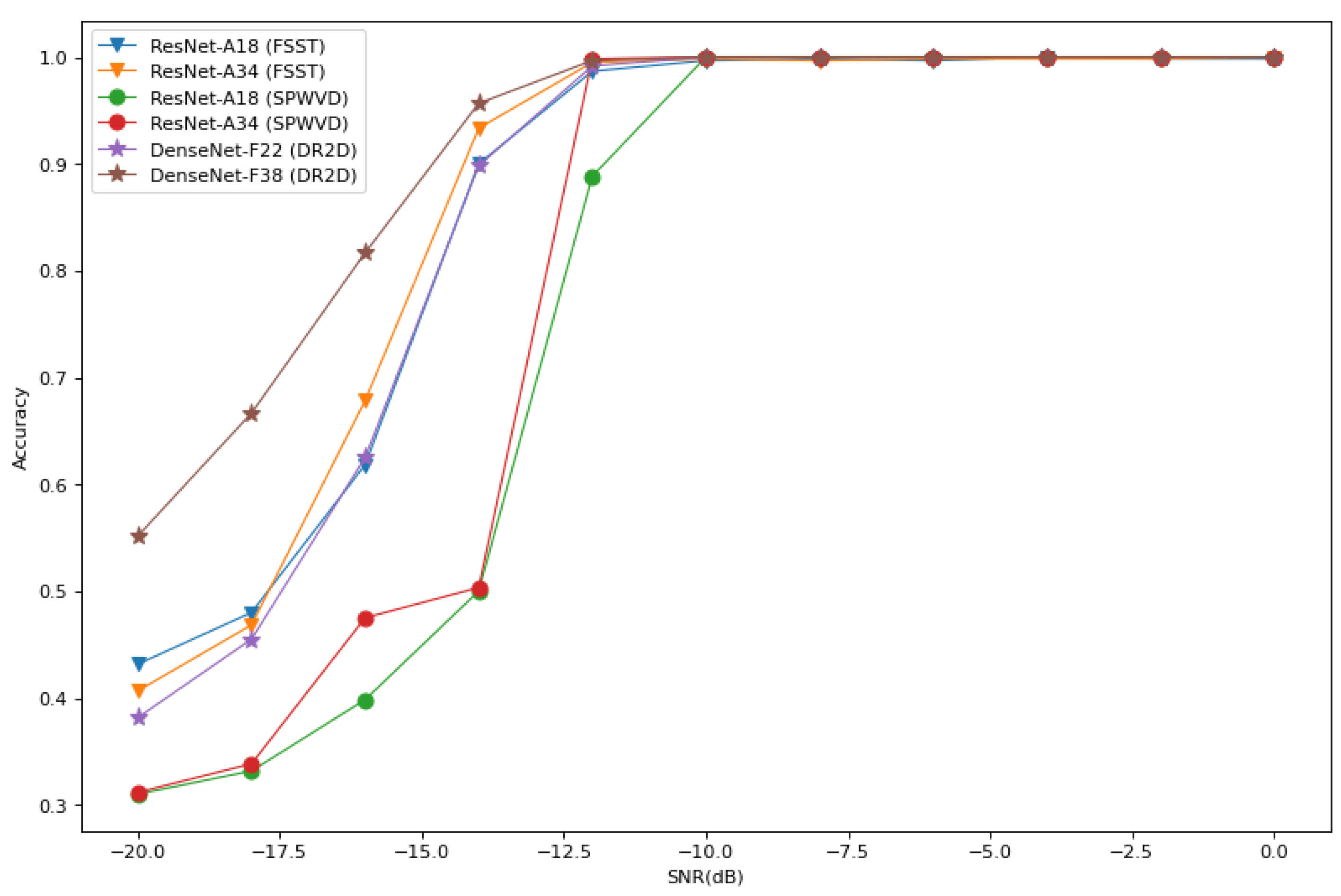
We constructed 18-layer and 34-layer CNNs integrating residual and attention connections as described in reference [15], denoted ResNet-A18 and ResNet-A34, respectively. In addition, we combined them with the FSST and SPWVD preprocessing methods for modulation recognition. We compared ResNet-A18 with DenseNet-22 and ResNet-18 combined with the FSST and SPWVD preprocessing methods, and the simulation results are shown in Figure 15. We also compared ResNet-A models combined with the FSST and SPWVD preprocessing methods with DenseNet-F models combined with the DR2D preprocessing method, and the simulation results are shown in Figure 16. Figure 15 shows that the recognition accuracy can be improved by changing the network architecture of the FSST preprocessing method. ResNet-A18, which adds attention connections to the ResNet-18 network architecture, had a higher average recognition accuracy than ResNet-18 and was comparable to DenseNet-22; however, it also had the largest numbers of parameters and FLOPs (12.6 M and 13.7274 × 10 9 , respectively), which greatly affected the recognition efficiency of the network. Moreover, changing the network architecture did not improve the recognition accuracy of the SPWVD preprocessing method. Figure 16 shows that the average recognition accuracy of DenseNet-F22 combined with the DR2D preprocessing method was comparable to that of ResNet-A18 with the FSST preprocessing method; for the network architecture proposed in reference [15], increasing the number of network layers did not significantly improve its accuracy. In contrast, increasing the number of network layers could significantly improve the accuracy of the DenseNet feature extraction network with early fusion proposed in this paper with the same growth rate. In summary, the preprocessing method utilized determined the upper recognition accuracy limit, while changing the network architecture had a limited effect on the attained recognition accuracy improvement. For AMR tasks, the priority was to choose an appropriate preprocessing method, and then a suitable feature recognition network could be selected according to the actual needs, such as the required inference time.

5. Conclusions

For the quick and accurate AMR of radiation source signals in cognitive radio systems, this paper proposes a DR2D preprocessing method for modulation feature extraction and constructs a DenseNet feature extraction network with early fusion to recognize the extracted features. The DR2D method has less computational complexity than time-frequency analysis methods and can produce three types of joint frequency feature bins for one radiation source signal in less time. The DenseNet feature extraction network with early fusion has fewer model parameters and FLOPs than other CNNs and is able to complete the recognition process in a short time. The simulation results show that DenseNet-F22 combined with the DR2D preprocessing method maintains an average recognition accuracy of more than 90% and a recognition accuracy of more than 60% for each modulation type in environments, with SNRs exceeding −14 dB. The model has good recognition performance in low-SNR environments. Furthermore, by comparing the recognition accuracies of multiple recognition networks with different preprocessing methods, we find that the upper recognition accuracy limit is determined by the selected preprocessing method rather than the network architecture; thus, it is very important to choose an appropriate preprocessing method before selecting a suitable feature recognition network for AMR tasks.

Author Contributions

Conceptualization, Y.L. and X.Y.; methodology, Y.L. and X.H.; software, Y.L.; validation, Y.L., G.Y. and D.H.; formal analysis, Y.L. and X.Y.; investigation, Y.L.; resources, X.Y. and X.H.; data curation, X.H.; writing—original draft preparation, Y.L. and X.Y.; writing—review and editing, Y.L. and X.Y.; visualization, G.Y. and D.H.; supervision, X.Y.; project administration, X.Y.; funding acquisition, X.Y. All authors have read and agreed to the published version of the manuscript.

Funding

This project was funded by the National Natural Science Foundation of China, grant numbers 61973037 and 61871414.

Data Availability Statement

The data are available from the corresponding author upon reasonable request.

Conflicts of Interest

The authors declare no conflict of interest.

Appendix A

Appendix A.1

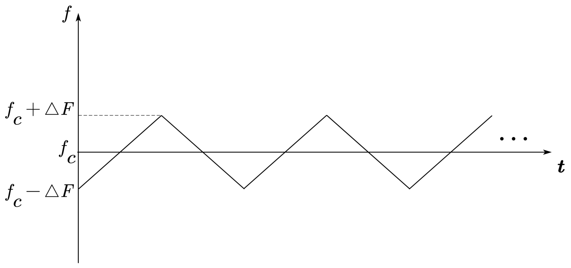
The model of a triangle wave frequency modulation signal can be expressed as follows:
s F M t = A F M cos { 2 π [ f c + ( 4 n + 1 ) Δ F ] t π β t 2 + φ 0 } , n T t n T + T 2 A F M cos { 2 π [ f c ( 4 n + 3 ) Δ F ] t + π β t 2 + φ 0 } , n T + T 2 t ( n + 1 ) T
where A F M is the carrier signal amplitude, f c is the carrier frequency, φ 0 is the initial phase angle, T is the modulation period, n = 0 , 1 , 2 , · · · is the number of the modulation period, and the frequency modulation slope can be defined as β = 4 Δ F / T . The frequency variation of the triangle wave frequency modulation signal is shown in Figure A1.
Figure A1. The frequency variation of the triangle wave frequency modulation signal.
Remotesensing 15 00518 g0a1

Appendix A.2

The model of a pulse amplitude modulation signal can be expressed as follows:
s P U L S E t = A P U L S E R [ t τ 0 ] cos ( 2 π f c t + φ 0 )
R t τ 0 = 1 , n T t n T + τ 0 0 , o t h e r s
where A P U L S E is the carrier signal amplitude, f c is the carrier frequency, φ 0 is the initial phase angle, T is the modulation period, n = 0 , 1 , 2 , · · · is the number of the modulation period, τ 0 is the pulse width, and R [ · ] is the periodic rectangular function.

Appendix A.3

The baseband signal of a binary phase shift keying signal can be expressed as follows:
p ( t ) = n = 0 i = 0 P 1 C i R t i T c n T T c
r e c t t T c = 1 , 0 t T c 0 , o t h e r s
where C i 0 , 1 is the binary code, T c is the code element width, n = 0 , 1 , 2 , · · · , P 1 is the number of the binary code in a modulation period, P is the total number of the binary code in a modulation period, T is the modulation period, n = 0 , 1 , 2 , · · · is the number of the modulation period, and r e c t [ · ] is the single rectangular function.
Then the model of a binary phase shift keying signal can be expressed as follows:
s B P S K t = A B P S K p ( t ) cos ( 2 π f c t + φ 0 )
where A B P S K is the carrier signal amplitude, f c is the carrier frequency, and φ 0 is the initial phase angle.

Appendix B

Appendix B.1

For a discrete signal s ( n ) , n = 0 , 1 , · · · , N 1 , the STFT is:
S T F T s g ( m , k ) = n = 0 M 1 s ( n ) g * ( n m N ) W M n k , k = 0 , 1 , · · · , M 1
where g ( n ) is a M-point time window, N is the step of the time window, and the exponent factor W M n k = e j 2 π M n k .
The local instantaneous frequency can be defined as follows:
Ω s g ( m , k ) = 1 2 π j Δ S T F T s g ( m , k ) S T F T s g ( m , k ) = k 1 2 π j S T F T s Δ m g ( m , k ) S T F T s g ( m , k )
where S T F T s Δ m g ( m , k ) denotes g (which is in S T F T s g ( m , k ) ), differentiate of the m.
The SST frequency redistribution operator is used to collect the dispersive time-frequency coefficients of the STFT:
T g , s ( m , l ) = k = 0 M 1 S T F T s g ( m , k ) W M m k δ i j ( l Ω s g ( m , k ) )
where δ i j ( · ) is the Kronecker function and the exponent factor W M m k = e j 2 π M m k can be integrated into (A7) for calculation.
The STFT processed by SST is referred to as the FSST.

Appendix B.2

For a discrete signal s ( n ) , n = 0 , 1 , · · · , N 1 , the WVD is:
W V D s ( m , k ) = n = N N s ( m + n / 2 ) s * ( m n / 2 ) W N n k
The SPWVD integrates two real-even windows into the WVD to smooth the time-frequency distribution for the time and frequency domains, respectively, which can be expressed as follows:
S P W V D s ( m , k ) = n = N N g ( m ) h ( k ) s ( m + n / 2 ) s * ( m n / 2 ) W N n k
where g ( m ) is the time window and h ( k ) is the frequency window.

References

  1. Azza, M.A.; Moussati, A.E.; Barrak, R. Implementation of Cognitive Radio applications on a Software Defined Radio plateform. In Proceedings of the 2014 International Conference on Multimedia Computing and Systems (ICMCS), Marrakech, Morocco, 14–16 April 2014; pp. 1037–1041. [Google Scholar] [CrossRef]
  2. Zhang, F.X.; Luo, C.B.; Xu, J.L.; Luo, Y.; Zheng, F.C. Deep learning based automatic modulation recognition: Models, datasets, and challenges. Digit. Signal Process. 2022, 129, 103650. [Google Scholar] [CrossRef]
  3. Benedetto, F.; Tedeschi, A.; Giunta, G. Automatic Blind Modulation Recognition of Analog and Digital Signals in Cognitive Radios. In Proceedings of the 2016 IEEE 84th Vehicular Technology Conference (VTC-Fall), Montréal, QC, Canada, 18–21 September 2016; pp. 1–5. [Google Scholar] [CrossRef]
  4. Zhu, M.T.; Li, Y.J.; Pan, Z.S.; Yang, J. Automatic modulation recognition of compound signals using a deep multi-label classifier: A case study with radar jamming signals. Signal Process. 2020, 169, 107393. [Google Scholar] [CrossRef]
  5. Lim, C.W.; Wakin, M.B. Automatic modulation recognition for spectrum sensing using nonuniform compressive samples. In Proceedings of the 2012 IEEE International Conference on Communications (ICC), Ottawa, ON, Canada, 10–15 June 2012; pp. 3505–3510. [Google Scholar] [CrossRef] [Green Version]
  6. Nasrallah, A.; Hamza, A.; Baudoin, G.; Toufik, B.; Zoubir, A.M. Simple improved mean energy detection in spectrum sensing for cognitive radio. In Proceedings of the 2017 5th International Conference on Electrical Engineering - Boumerdes (ICEE-B), Boumerdes, Algeria, 29–31 October 2017; pp. 1–4. [Google Scholar] [CrossRef]
  7. Kozal, A.S.B.; Merabti, M.; Bouhafs, F. An improved energy detection scheme for cognitive radio networks in low SNR region. In Proceedings of the 2012 IEEE Symposium on Computers and Communications (ISCC), Cappadocia, Turkey, 1–4 July 2012; pp. 000684–000689. [Google Scholar] [CrossRef]
  8. Xu, J.L.; Su, W.; Zhou, M. Likelihood-Ratio Approaches to Automatic Modulation Classification. IEEE Trans. Syst. Man Cybern. Part C (Appl. Rev.) 2011, 41, 455–469. [Google Scholar] [CrossRef]
  9. Wang, F.; Wang, X. Fast and Robust Modulation Classification via Kolmogorov-Smirnov Test. IEEE Trans. Commun. 2010, 58, 2324–2332. [Google Scholar] [CrossRef]
  10. Hazza, A.; Shoaib, M.; Alshebeili, S.A.; Fahad, A. An overview of feature-based methods for digital modulation classification. In Proceedings of the 2013 1st International Conference on Communications, Signal Processing, and Their Applications (ICCSPA), Sharjah, United Arab Emirates, 12–14 February 2013; pp. 1–6. [Google Scholar] [CrossRef]
  11. Liu, S.K.; Yan, X.P.; Li, P.; Hao, X.H.; Wang, K. Radar Emitter Recognition Based on SIFT Position and Scale Features. IEEE Trans. Circuits Syst. II Express Briefs 2018, 65, 2062–2066. [Google Scholar] [CrossRef]
  12. Quan, D.Y.; Tang, Z.Y.; Wang, X.F.; Zhai, W.C.; Qu, C.X. LPI Radar Signal Recognition Based on Dual-Channel CNN and Feature Fusion. Symmetry 2022, 14, 570. [Google Scholar] [CrossRef]
  13. Rueda, A.; Krishnan, S. Augmenting Dysphonia Voice Using Fourier-based Synchrosqueezing Transform for a CNN Classifier. In Proceedings of the ICASSP 2019-2019 IEEE International Conference on Acoustics, Speech and Signal Processing (ICASSP), Brighton, UK, 12–17 May 2019; pp. 6415–6419. [Google Scholar] [CrossRef]
  14. Kong, G.; Jung, M.; Koivunen, V. Waveform Classification in Radar-Communications Coexistence Scenarios. In Proceedings of the GLOBECOM 2020 - 2020 IEEE Global Communications Conference, Taipei, Taiwan, 7–11 December 2020; pp. 1–6. [Google Scholar] [CrossRef]
  15. Huynh-The, T.; Pham, Q.V.; Nguyen, T.V.; Kim, D.S. Deep Learning for Coexistence Radar-Communication Waveform Recognition. In Proceedings of the 2021 International Conference on Information and Communication Technology Convergence (ICTC), Jeju Island, Republic of Korea, 20–22 October 2021; pp. 1725–1727. [Google Scholar] [CrossRef]
  16. Su, L.; Wu, H.S.; Tzuang, C.K.C. 2-D FFT and time-frequency analysis techniques for multi-target recognition of FMCW radar signal. In Proceedings of the Asia-Pacific Microwave Conference 2011, Melbourne, VIC, Australia, 5–8 December 2011; pp. 1390–1393. [Google Scholar]
  17. Chin, H.Y.; Tsai, P.Y.; Lee, S.Y. Implementation of a Two-Dimensional FFT/IFFT Processor for Real-Time High-Resolution Synthetic Aperture Radar Imaging. In Proceedings of the 2021 IEEE Workshop on Signal Processing Systems (SiPS), Coimbra, Portugal, 19–21 October 2021; pp. 211–216. [Google Scholar] [CrossRef]
  18. Auger, F.; Flandrin, P.; Lin, Y.T.; McLaughlin, S.; Meignen, S.; Oberlin, T.; Wu, H.T. Time-Frequency Reassignment and Synchrosqueezing: An Overview. IEEE Signal Process. Mag. 2013, 30, 32–41. [Google Scholar] [CrossRef] [Green Version]
  19. Oberlin, T.; Meignen, S.; Perrier, V. The fourier-based synchrosqueezing transform. In Proceedings of the 2014 IEEE International Conference on Acoustics, Speech and Signal Processing (ICASSP), Florence, Italy, 4–9 May 2014; pp. 315–319. [Google Scholar] [CrossRef] [Green Version]
  20. Kalra, M.; Kumar, S.; Das, B. Target Detection Using Smooth Pseudo Wigner-Ville Distribution. In Proceedings of the 2018 IEEE Recent Advances in Intelligent Computational Systems (RAICS), Thiruvananthapuram, India, 6–8 December 2018; pp. 6–10. [Google Scholar] [CrossRef]
  21. Ting, Z.; Lin, Y.; Jishen, L.; Chengxiang, Z. A High Quality Time-Frequency Analysis Method. In Proceedings of the 2022 7th International Conference on Computer and Communication Systems (ICCCS), Wuhan, China, 22–25 April 2022; pp. 344–348. [Google Scholar] [CrossRef]
  22. He, K.; Zhang, X.; Ren, S.; Sun, J. Deep Residual Learning for Image Recognition. In Proceedings of the 2016 IEEE Conference on Computer Vision and Pattern Recognition (CVPR), Las Vegas, NV, USA, 27–30 June 2016; pp. 770–778. [Google Scholar] [CrossRef] [Green Version]
  23. Huang, G.; Liu, Z.; Maaten, L.V.D.; Weinberger, K.Q. Densely Connected Convolutional Networks. In Proceedings of the 2017 IEEE Conference on Computer Vision and Pattern Recognition (CVPR), Honolulu, HI, USA, 21–26 July 2017; pp. 2261–2269. [Google Scholar] [CrossRef] [Green Version]
  24. Huang, G.; Liu, Z.; Pleiss, G.; Maaten, L.v.d.; Weinberger, K.Q. Convolutional Networks with Dense Connectivity. IEEE Trans. Pattern Anal. Mach. Intell. 2022, 44, 8704–8716. [Google Scholar] [CrossRef] [PubMed] [Green Version]
  25. Duhamel, P.; Vetterli, M. Fast Fourier transforms: A tutorial review and a state of the art. Signal Process. 1990, 19, 259–299. [Google Scholar] [CrossRef]
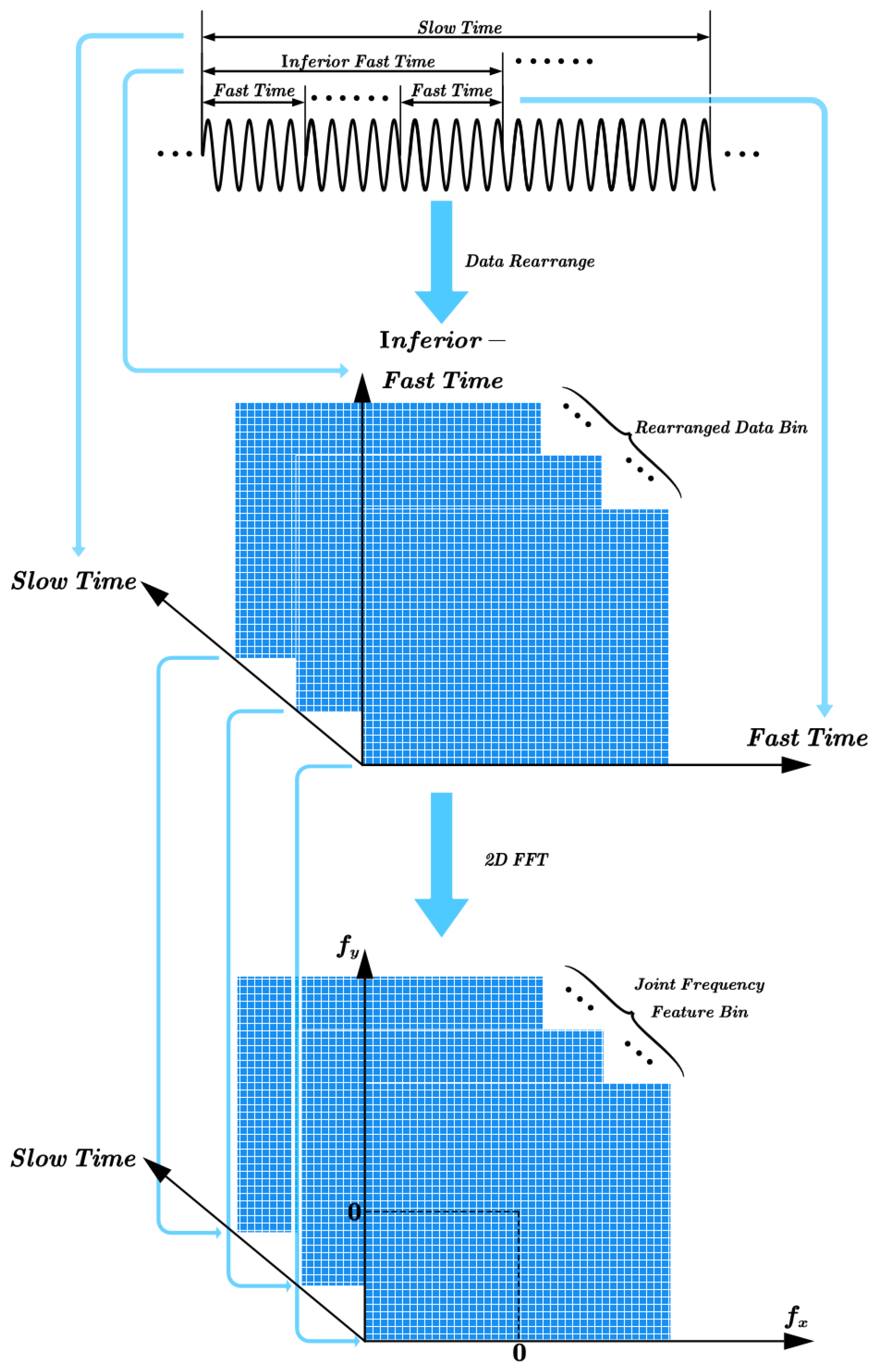
Figure 1. Modulation feature extraction based on DR2D.
Remotesensing 15 00518 g001
Figure 2. Two-Dimensional FFT of the data slice.
Remotesensing 15 00518 g002
Figure 3. Image of texture features of the data slice.
Remotesensing 15 00518 g003
Figure 4. DR2D features of typical radiation source signals. (a) DRP of a continuous wave signal; (b) ORP of a continuous wave signal; (c) DRP of a triangle wave frequency modulation signal; (d) ORP of a triangle wave frequency modulation signal; (e) DRP of a pulse amplitude modulation signal; (f) ORP of a pulse amplitude modulation signal; (g) DRP of a binary phase shift keying signal; (h) ORP of a binary phase shift keying signal.
Remotesensing 15 00518 g004aRemotesensing 15 00518 g004b
Figure 5. Feature analysis of the signals overlapping in the frequency domain. (a) FSST (20 dB); (b) FSST (−15 dB); (c) SPWVD (20 dB); (d) SPWVD (−15 dB); (e) DR2D (20 dB); (f) DR2D (−15 dB).
Remotesensing 15 00518 g005aRemotesensing 15 00518 g005b
Figure 6. Feature images of triangle wave frequency modulation signals with different relative bandwidths. (a) SPWVD ( f f o c = 0.02 ); (b) SPWVD ( f f o c = 0.04 ); (c) SPWVD ( f f o c = 0.08 ); (d) DR2D ( f f o c = 0.02 ); (e) DR2D ( f f o c = 0.04 ); (f) DR2D ( f f o c = 0.08 ).
Remotesensing 15 00518 g006aRemotesensing 15 00518 g006b
Figure 7. Feature recognition process of the DenseNet feature extraction network with early fusion.
Remotesensing 15 00518 g007
Figure 8. DR2D preprocessing of the radiation source signal.
Remotesensing 15 00518 g008
Figure 9. 4-layer dense block.
Remotesensing 15 00518 g009
Figure 10. Transition layer.
Remotesensing 15 00518 g010
Figure 11. The structure of DenseNet-F22.
Remotesensing 15 00518 g011
Figure 12. The training and testing loss curves and the corresponding accuracy curves versus the number of epochs.
Remotesensing 15 00518 g012
Figure 13. The average recognition accuracy curves of DenseNet-F22, DenseNet-22, and ResNet-18 feature recognition networks in environments with different SNRs.
Remotesensing 15 00518 g013
Figure 14. The recognition accuracy achievements for each modulation type in environments with different SNRs.
Remotesensing 15 00518 g014
Figure 15. The average recognition accuracy curves of ResNet-A18, DenseNet-22, and ResNet-18 combined with the FSST and SPWVD preprocessing methods in environments with different SNRs.
Remotesensing 15 00518 g015
Figure 16. The average recognition accuracy curves produced with different numbers of layers for the DenseNet-F models and ResNet-A models proposed in reference [15] in environments with different SNRs.
Remotesensing 15 00518 g016
Table 1. Computational complexities of the DR2D, FSST and SPWVD preprocessing methods.
Preprocessing MethodDR2DFSSTSPWVD
Computational complexity O [ 2 n × 2 n a log 2 ( 2 n a ) + 16 × 2 × n 4 × n a 2 log 2 n a 2 + 64 × 2 × n 8 × n a 4 log 2 n a 4 ] = O [ 4 n n a ( 3 log 2 n a 2 ) ] O ( n 2 32 × n a log 2 n a + n 2 32 × n a ) = O [ n 2 n a 32 ( l o g 2 n a + l ) ] O [ n 2 32 × 2 n a log 2 ( 2 n a ) + n 2 32 × ( n a 2 + n a + n a ) ] = O [ n 2 n a 32 ( 2 log 2 n a + n a + 4 ) ]
Table 2. Network architectures of DenseNet-F22, DenseNet-22 and ResNet-18.
Layers
(DenseNet)
DenseNet-F22DenseNet-22ResNet-18Layers
(ResNet)
-Input Size (1):Input Size (1):Input Size (1):-
1 × 448 × 448 1 × 224 × 224 1 × 224 × 224
Convolution 7 × 7 conv, stride 2Convolution
(Output Size: 16 × 224 × 224 )(Output Size: 32 × 112 × 112 )(Output Size: 1 × 112 × 112 )
Pooling 3 × 3 max pooling, stride 2- 3 × 3 max pooling, stride 2Pooling
(Output Size: 16 × 112 × 112 )(Output Size: 1 × 56 × × 56 )
-Input Size (2):---
32 × 112 × 112 (concat)
Convolution 3 × 3 conv, stride 2 3 × 3 conv, stride 2--
(Output Size: 64 × 56 × 56 )(Output Size: 128 × 56 × 56 )
-Input Size (3):---
128 × 56 × 56 (concat)
Dense [ 3 × 3 conv ] × 4 , k = 32 3 × 3 conv , 64 3 × 3 conv , 64 ×2Residual
Block (1)(Output Size: 256 × 56 × 56 )(Output Size: 64 × 56 × 56 )Block (1)
1 × 1 conv--
Transition(Output Size: 128 × 56 × 56 )
Layer (1) 2 × 2 average pooling, stride 2
(Output Size: 128 × 28 × 28 )
Dense [ 3 × 3 conv ] × 4 , k = 32 3 × 3 conv , 128 3 × 3 conv , 128 × 2 Residual
Block (2)(Output Size: 256 × 28 × 28 )(Output Size: 128 × 28 × 28 )Block (2)
1 × 1 conv--
Transition(Output Size: 128 × 28 × 28 )
Layer (2) 2 × 2 average pooling, stride 2
(Output Size: 128 × 14 × 14 )
Dense [ 3 × 3 conv ] × 4 , k = 32 3 × 3 conv , 256 3 × 3 conv , 256 ×2Residual
Block (3)(Output Size: 256 × 14 × 14 )(Output Size: 256 × 14 × 14 )Block (3)
1 × 1 conv--
Transition(Output Size: 128 × 14 × 14 )
Layer (3) 2 × 2 average pooling, stride 2
(Output Size: 128 × 7 × 7 )
Dense[ 3 × 3  conv] × 4 , k = 32 3 × 3 conv , 512 3 × 3 conv , 512 × 2 Residual
Block (4)(Output Size: 256 × 7 × 7 )(Output Size: 512 × 7 × 7 )Block (4)
7 × 7 global average pooling 7 × 7 global average pooling
Classification(Output Size: 256 × 1 × 1 )(Output Size: 512 × 1 × 1 )Classification
flatten
Layer256-D fully connected,512-D fully connected,Layer
softmaxsoftmax
Params0.9 M1.0 M11.2 MParams
FLOPs 1.0974 × 10 9 1.1386 × 10 9 1.7473 × 10 9 FLOPs
Table 3. The parameters of different radiation source signals.
Modulation TypeCF (GHz)MF (KHz)FD (MHz)PW (ns)DCEW (ns)
CW[1, 5]-----
TRIFM[1, 5][200, 500][100, 200]---
SINFM[1, 5][200, 500][100, 200]---
PAM[1, 5]--[40, 70][1%, 4%]-
BPSK[1, 5]----[50, 80]
LFM_PULSE[1, 5]-[20, 40][200, 500][20%, 33%]-
Disclaimer/Publisher’s Note: The statements, opinions and data contained in all publications are solely those of the individual author(s) and contributor(s) and not of MDPI and/or the editor(s). MDPI and/or the editor(s) disclaim responsibility for any injury to people or property resulting from any ideas, methods, instructions or products referred to in the content.