Point Cloud Plane Segmentation-Based Robust Image Matching for Camera Pose Estimation

Abstract

The mainstream image matching method for recovering the motion of the camera is based on local feature matching, which faces the challenges of rotation, illumination, and the presence of dynamic objects. In addition, local feature matching relies on the distance between descriptors, which easily leads to lots of mismatches. In this paper, we propose a new robust image matching method for camera pose estimation, called IM_CPE. It is a novel descriptor matching method combined with 3-D point clouds for image matching. Specifically, we propose to extract feature points based on a pair of matched point cloud planes, which are generated and segmented based on depth images. Then, the feature points are matched based on the distance between their corresponding 3-D points on the point cloud planes and the distance between their descriptors. Moreover, the robustness of the matching can be guaranteed by the centroid distance of the matched point cloud planes. We evaluate the performance of IM_CPE using four well-known key point extraction algorithms, namely Scale-Invariant Feature Transform (SIFT), Speed Up Robust Feature (SURF), Features from Accelerated Segment Test (FAST), and Oriented FAST and Rotated Brief (ORB), with four sequences from the TUM RGBD dataset. According to the experimental results, compared to the original SIFT, SURF, FAST, and ORB algorithms, the NN_mAP performance of the four key point algorithms has been improved by 11.25%, 13.98%, 16.63%, and 10.53% on average, respectively, and the M.Score has also been improved by 25.15%, 23.05%, 22.28%, and 11.05% on average, respectively. The results show that the IM_CPE can be combined with the existing key points extraction algorithms and the IM_CPE can significantly improve the performance of these key points algorithms.

1. Introduction

The motion of the camera can be recovered by the correspondence between a series of images, which plays an important role on some multiple-view-geometry-based computer vision tasks such as structure-from-motion (SfM), 3-D reconstruction, and simultaneous localization and mapping (SLAM). To find the correspondences between images, the local features of the images are matched based on the distance between the descriptors of the features. This image matching progress is also known as the feature points matching. Feature point matching is challenging for images with large angle rotation, fast movement, and changes in scale and illumination. Thus, in recent years, lots of matching methods have been proposed to improve the performance of image matching. The existing feature points matching methods can be roughly categorized into two categories: descriptor matching with mismatch removal and learning-based matching.

Descriptor matching with mismatch removal usually casts the tasks into a two-step problem. The first step is to measure the distance of the descriptors to find the corresponding key points by matching strategies such as a fixed threshold, nearest neighbor (NN), mutual nearest neighbor, and nearest neighbor distance ratio [1]. In the scenario of a fixed threshold matching strategy, feature points are matched if the distance between their descriptor is below a fixed threshold. Mikolajczyk et al. [2] concluded that, with this approach, one descriptor could be matched several times and the accuracy cannot be guaranteed. The nearest neighbor strategy defines that if one descriptor is the nearest neighbor to another descriptor while the distance between the two descriptors is below a certain threshold, the two descriptors can be regarded as matched. Since one descriptor only has one nearest neighbor, with this approach, one descriptor has only one match. The nearest neighbor distance ratio is similar to the nearest neighbor method except that the threshold of the distance depends on the ratio between the first- and the second-nearest neighbor. Mikolajczyk et al. [2] also conducted experiments to evaluate the performance of these three strategies on the Scale-Invariant Feature Transform (SIFT) [3] descriptor and SIFT-like descriptors. They gave a conclusion that the nearest-neighbor-based matching strategy performs better than the fixed threshold stategy because the nearest neighbor strategies select only the best candidate match and reject all the other matches.

Histogram of gradient (HoG) descriptors, such as SIFT [3], Speed Up Robust Feature (SURF) [4], Principle Components Analysis SIFT (PCA-SIFT) [5], and Learned Invariant Feature Transform (LIFT) [6], use the L2-Norm to measure the distance of the descriptors in measuring space. This is usually a high-dimensional floating-point operation and requires lots of calculation resources. Binary descriptors such as binary robust independent elementary features (BRIEFs) [7], binary robust invariant scalable keypoints (BRISKs), and rotated binary robust independent elementary features (rBRIEFs) [8] were further proposed to use the Hamming distance [9] instead of the L2-Norm to measure the similarity of the descriptors, which improved the performance of traditional image matching pipeline.

However, the use of only local descriptors and the similarity measurement of the descriptors will unavoidably result in a large number of incorrect matches, particularly when images undergo a serious non-rigid deformation, a large angle of rotation, and fast movement. Since it is difficult to further improve the matching strategy, several mismatch removal methods have been proposed based on the existing matching result to preserve as many correct matches as possible while keeping the mismatch to a minimum. Thereafter, the mismatched descriptor will be removed based on extra constraints by the random sample consensus (RANSAC) [10] algorithm. The RANSAC algorithm filters the qualified inliers and outliers by randomly selecting the input observation data and fitting a certain mathematical model. The essential matrix of two images describes the relationship between the 3-D points of a scene and the image coordinates of different cameras. Since there are 5 degrees of freedom in the essential matrix, it needs at least five pairs of matched points to estimate the matrix [11]. However, using only five pairs of matched points for estimation takes lots of calculation resources. Hartley et al. suggested using eight pairs of points [12] and seven pairs of points [13] to estimate the essential matrix. With the estimation method of essential matrix, RANSAC is applied to image matching tasks. It randomly selects the matched feature points, calculates the essential matrix, and then calculates the reprojection error between all points in the dataset and the model. The points with the smallest errors are recorded as the optimal inliers, which can be regarded as the well-matched feature points, and the reprojection model with the largest number of inliers can be regarded as the best model.

With the development of deep learning, learning-based matching methods have been proposed. Some methods realize learning for matching images without attempting to detect the structure of the images a priori. Revaud et al. [14] proposed a deep matching approach that has a good performance in non-rigid deformations and repetitive textures and efficiently determines dense correspondences in the presence of significant changes between images. Arar et al. [15] proposed an unsupervised multi-modal registration method using two networks, a spatial transformation network, and a translation network, which bypass the difficulties of developing cross-modality similarity measures. DeTone et al. [16] changed the traditional inherent process of pose estimation from feature matching. They directly estimated the projective model and the Homography matrix from image pairs by a fully convolutional network. Similarly, Poursaeed et al. [17] estimated the fundamental matrix from image pairs, and Rocco et al. [18] estimated the non-rigid deformation. In addition to these learning methods from images and image patch methods, the points-based learning method has received increasing consideration. Brachmann et al. [19] first proposed a differentiable RANSAC (DSAC), which is inspired by reinforcement learning to use probability to select the deterministic hypothesis to overcome the problem that RANSAC [10] is non-differentiable and can not be used in a deep learning pipeline.

As one type of 3-D data, the point clouds are widely used in SLAM, autopilot, and augmented reality. Point cloud data obtained from devices, such as LiDAR and RGBD cameras, generally need to be registered before they can be used. At present, the traditional mainstream point cloud registration technology mainly includes two categories: coarse registration and fine registration. The coarse registration stage is to make the two point clouds roughly aligned for any initial state of the two point clouds and to provide initial values for the rotation matrix R and the translation vector T. Aiger et al. proposed a 4-points congruent sets (4PCS) algorithm based on RANSAC [10] for the purpose of coarse registration. Rusu et al. proposed point feature histograms (PFHs) [20] and fast point feature histograms (FPFHs) [21] to extract geometric features from point clouds. Based on FPFH, a lot of point cloud registration methods have been proposed, such as sample consensus initial alignment (SAC-IA) [21], truncated least squares estimation and semidine relaxation (TEASER) [22], and fast global registration [23]. However, fine registration uses the result of the coarse matching as an initial transformation and performs more accurately than coarse registration. Besl et al. [24] proposed an iterate closest point (ICP) algorithm to iterate the closest point in the point cloud and obtain the transformation model, which can get a minimal loss function. Since the ICP algorithm is prone to fall into a local optimum, many state-of-the-art methods have been proposed to improve the performance of point cloud registration.

In general, to improve the performance of image matching methods is to extract more robust descriptors and remove the mismatch. In this paper, we propose a new robust image matching method for camera pose estimation, called IM_CPE. IM_CPE is a novel descriptor matching method combined with a 3-D point cloud for image matching. The 2-D feature points will be extracted on pairs of matched point cloud planes, which are extracted and matched based on depth images. Then, the feature points will be coarsely matched if the Euclidean distance of the corresponding 3-D points of the feature points is below the centroid distance of the matched point cloud planes. Finally, according to the result of coarse matching, the descriptors of the 2-D feature points are matched for fine matching. The key contributions are summarized as follows:

• Differing from the previous RGB-image-based descriptor matching methods, we use depth images corresponding to RGB images as an extra constraint. We transform the depth images into point clouds to measure the relative position relationship between pixels from RGB images in 3-D spaces.
• Differing from the previous nearest neighbor descriptor matching methods, we propose a descriptor matching approach with a coarse matching strategy for image matching. The coarse matching step is based on the Euclidean distance between the feature points on a pair of matched point cloud planes in 3-D shapes. If the Euclidean distance is below the centroid distance of the matched point cloud planes, the descriptors of the feature points are calculated for fine matching.
• Differing from the previous full image matching methods, we propose to segment the image into several blocks and match the blocks from the different images in advance. Then, the feature points can be extracted and matched based on the already matched image blocks. To achieve this goal, we transform the depth image into point clouds and then segment the point cloud planes to simulate the image block. As the area of searchable matched feature points becomes smaller, the probability of feature matching error also decreases.
• We propose a point cloud plane segmentation (PCPS) algorithm to segment planes from point clouds, and a point cloud plane matching (PCPM) algorithm to coarsely match two planes based on the centroid distance and angle of two cloud point planes.
• We propose a key point mapping (KMAP) algorithm to map the 2-D feature points into 3-D shapes. Using coarse matching and fine matching, a key point matching (KMAT) algorithm determines whether the two feature points from matched point cloud planes in 3-D shapes are a potential correspondence, based on the Euclidean distance of these points and the centroid distance between the plane they belong to.

In the following sections, Section 2 introduces and discusses related works in recent years. The proposed robust image matching method will be introduced in Section 3. The experimental results and analysis to show the performance of the proposed method are given in Section 4. Discussions are provided in Section 5 and finally conclusions are included in Section 6.

2. Related Works

In recent years, many researchers have focused on how to improve the performance of the traditional image matching pipeline. Torr et al. [25] proposed a method called MLESAC to evaluate the estimated model quality by a maximum likelihood process rather than just the number of inliers. The experiment results indicate that MLESAC can improve the results under certain assumptions. Tordoff et al. [26] observed that RANSAC [10] runs much longer than the theoretically predicted value. Chum et al. [27] considered that this discrepancy is due to the incorrect assumption that a model with parameters computed from an outlier-free sample is consistent with all inliers, which rarely holds in practice. To address this discrepancy, Chum et al. [27] proposed a locally optimized RANSAC (LO-RANSAC) to improve the performance for finding inliers and the speed of the RANSAC procedure by applying a local optimization. The experiment result showed that the performance of LO-RANSAC is increased by 10%-20% more than RANSAC in some tasks such as epipolar geometry and homography estimation. Barath et al. [28] proposed a Graph-Cut RANSAC (GC-RANSAC), which introduced a graph-cut algorithm into the local optimization step to improve LO-RANSAC [27]. The experiment results indicate that GC-RANSAC performs better than state-of-the-art methods for a range of problems. Chum et al. [29] proposed a progressive sample consensus (PROSAC) algorithm. Compared to RANSAC, PROSAC orders the dataset by linear ordering through a similarity function and draws the PROSAC sample from a progressively increased dataset of correspondences with good performance. The experiment result indicates that PROSAC is much faster than RANSAC in most cases. Meanwhile, the performance of PROSAC converges towards RANSAC even in the worst case. Chung et al. [30] proposed an effective cooperative random sample consensus (COOSAC) based on the geometry histogram as a variant method of RANSAC for image matching. The experiment results indicate that the proposed COOSAC has decreased the computational cost compared to RANSAC and produces a better matching result. In addition to RANSAC and its variants algorithm, Bian et al. [31] proposed grid-based motion statistics (GMS). This approach introduced motion smoothness as the statistical measure to reject false matches, which has been validated to perform better in experiments. Liu et al. [32] proposed a matched image pairs selection algorithm for SfM based on the graph-indexed bag-of-words (BoW) model (GIBoW). The experiment result indicates that the GIBoW-based method improves the efficiency of image match pair selection.

The deep-learning-based matching method focuses on learning from putative correspondences and finding good correspondences from them. Brachmann et al. [33] proposed a neural-guided RANSAC (NG-RANSAC), which is a self-supervised learning method that uses the inlier count itself as a training objective. In addition, many researchers propose to treat this task as a classification task. Yi et al. [34] trained a deep network to solve a classification problem and a regression problem. The former is to determine whether a correspondence is good and the latter is to estimate the essential matrix. The experiment result indicated that this approach improves the existing image matching method on multiple challenging datasets with little training data. Similar to [34], Zhang et al. [35] proposed an order-aware network to calculate the probability of a putative correspondence to be an inlier and estimate the essential matrix. This approach first clusters the unordered input putative correspondences to obtain the local context and then exploits the complex global context of the putative correspondences. The experiment result indicated that the accuracy of the relative pose estimation improved significantly. Ma et al. [36] proposed to train a two-class classifier for mismatch removal. This classifier constructed a handcrafted geometrical representation for each putative correspondence for training on datasets with few images and has shown promising matching performance with generality and robustness. In addition, for some specific scenarios, Quan et al. [37] proposed a 3-D convolutional neural network to enhance the quality of feature extraction and matching in the low-light image for SLAM. The experiment result indicated that the proposed method provided a lower positioning error and root mean squared error on the TUM VI dataset.

For point cloud registration, Pavlov et al. [38] introduced the Anderson algorithm into ICP to improve the robustness and speed. Different from ICP, Magnusson et al. [39] proposed a 3-D normal distributions transformation (NDT) inspired by 2-D NDT [40]. This method splits the point cloud data into block-sized grids or voxels, fits a normal distribution model in each grid, and finally uses the Newton optimization algorithm to optimize the parameters. Similar to ICP, NDT still requires a good initial pose; otherwise, it is also easy to fall into local extrema. Liu et al. [41] proposed to use FPFH [21] and Hausdorff distance to search for corresponding 3-D points in the point cloud for coarse registration and an improved NDT for fine registration. Steder et al. [42] proposed a normal aligned radial feature (NARF) to extract feature points from surface stable regions and object edges and then use the Manhattan distance for coarse registration. To improve the performance of point cloud registration, Zhang et al. [43] proposed a point cloud rectification method based on laser intensity. They interpolate the intensity data to generate laser intensity images and then apply a non-linear least square algorithm to solve the boresight angular error parameters. The experiment result indicates that this method has decreased the average planar root mean square error (RMSE) by 1.1 cm and elevation RMSE by 0.8 cm compared to the stepwise geometric method.

There are several methods that have been proposed to estimate planes from point clouds. Alexa et al. [44] proposed to use ordinary least square (OLS) to find a plane. OLS requires all points in point clouds to have the minimum distance to the modeled plane and it seeks the best plane equation by minimizing the sum of squares of errors. In addition, RANSAC [10] can also be used to model the plane of point clouds. RANSAC obtains a plane by randomly selecting three points in the point cloud and calculates the distance between all points and the plane. If the distance between the point and the plane is less than a certain threshold, the point is considered as an inlier, and inliers are counted. RANSAC repeats the above steps until a maximum number of total inliers is obtained. At this time, the plane equation will be considered the optimal equation. PROSAC [29] is one of the variants of RANSAC, and it is also usually used in point cloud plane estimation. The difference between PROSAC and RANSAC is that PROSAC sorts the points by a quality measurement, and each iteration only chooses the points with high quality.

3. Robust Image Matching Method for Camera Pose Estimation (IM_CPE)

This section describes the proposed approach, IM_CPE, in detail. In order to derive more accurate corresponding key points from two images, in this work, we propose a KMAP algorithm to extract the 3-D coordinate key points and a KMAT algorithm to match the key points. To fulfill the key points matching, the point cloud plane segmentation (PCPS) and point cloud plane matching (PCPM) algorithms are proposed to generate the matched point cloud planes.

Figure 1 shows the flowchart of the proposed IM_CPE. Given two adjacent RGB images $I_A$ and $I_B$, with their corresponding depth images $D_A$ and $D_B$, firstly the KMAP algorithm is applied to $I_A$ and $I_B$, to extract the 3-D coordinate key points $K_A$ and $K_B$. Simultaneously, the proposed PCPS algorithm is applied to $D_A$ and $D_B$ to segment the point cloud planes by Euclidean clustering. Then, the PCPS algorithm models the segmented point cloud planes ${\mathrm{\Pi }}_A^i$ and ${\mathrm{\Pi }}_B^j$ to gain the plane equations and further estimate the normal vector L and centroid G of the planes. After L and G are calculated, the proposed PCPM algorithm matches two point cloud planes if the centroid of a plane from ${\mathrm{\Pi }}_A^i$ is the closet to another centroid from ${\mathrm{\Pi }}_B^j$ and the angle of the normal vector of the planes is the smallest. With the point cloud planes matched, the KMAT algorithm is proposed to determine which planes the key points from $K_A$ and $K_B$ belong to. Next, the Euclidean distance $dis{t}_M$ of two 3-D key points on a pair of matched planes is calculated for coarse matching. If $dis{t}_M$ is below the distance between the centroid of the matched planes, the two key points can be regarded as a potential match and the descriptors of the two key points are calculated for fine matching.

In the proposed KMAP algorithm, the key points with their 2-D coordinates are extracted from $I_A$ and $I_B$, which are then mapped into 3-D coordinates, notated as $K_A$ and $K_B$, respectively. In the proposed PCPS, the depth values are extracted from the depth image $D_A$ and $D_B$, according to which, the point cloud $P_A$ and $P_B$ are generated by mapping pixels into the 3-D point cloud P. In the proposed PCPM, the point cloud planes will be matched based on the normal vectors L and centroid G, and the distance $d_G$ between the centroid of the matched planes will be calculated. In the proposed KMAT, the distance $d_M$ between two key points in 3-D shapes that are from a pair of matched planes will be calculated for coarse matching. If $d_M<d_G$, the descriptors of the pair of points will be calculated for fine matching.

In the following subsections, Section 3.1 introduces the proposed PCPS and PCPM and Section 3.2 explains the proposed KMAP and KMAT in detail.

3.1. Point Cloud Plane Segmentation and Matching

In the proposed IM_CPE, we first propose a PCPS and PCPM algorithm to segment and match the point cloud plane to generate putative corresponding image patches for key point extraction and matching. In previous years, researchers usually focused on full-size images, and brute-force matched two key points according to the distance between their descriptors. In addition, a traditional algorithm, such as SIFT [3], SURF [4], and ORB [8], usually uses an experience distance value as a threshold to filter the matched key points; as a consequence, the matching accuracy rate of the key points may be quite low in some scenarios, such as large angle rotation, fast movement, and so on. We assume that a full image matching progress can be replaced by extracting and matching key points on several small already matched image blocks at the same time, and the performance of key points matching can be improved. To achieve this goal, we extract and match point cloud planes based on depth images to simulate the matched image blocks and extract image key points based on the matched point cloud planes due to the fact that the image blocks directly extracted from RGB images are hard to match. To segment and match planes from the real world, we use depth images to transform the 2-D RGB images back to 3-D coordinates to simulate the real world, which means every pixel in an RGB image will be transformed into a 3-D point and be represented by a point cloud. Thus, we propose a PCPS and PCPM algorithm, which can segment point cloud planes and match them based on a given pair of depth images. Afterwards, the key points from the matched planes can be matched based on the distance between their corresponding 3-D points and the distance of their descriptors.

A pixel on a depth image can be represented as $p={[u,v]}^T$, and the value of this pixel equals d. A 3-D point $P={[X,Y,Z]}^T$, which corresponds to p, can be calculated by the following:

$$\left\{\begin{array}{c}Z=d\hfill \\ X=(u-c_x)·d/f_x\hfill \\ Y=(v-c_y)·d/f_y\hfill \end{array}\right.$$

(1)

where the $c_x$, $c_y$, $f_x$, and $f_y$ are the camera intrinsics, which are provided by camera manufacturers. After iteration through all points on the depth image and processing by (1), point clouds $P_A$ and $P_B$ are thus generated.

Because the original point clouds contain a large number of points, which has a great impact on the accuracy and speed of the IM_CPE algorithm, we employ a voxel grid filter to downsample the generated point clouds $P_A$ and $P_B$, which has the ability to reduce the number of point clouds while preserving the shapes of the point cloud. In addition, since there are lots of noise points and sparsely distributed points in the original point clouds, the accuracy of centroid estimation and plane estimation is affected by these points. Eliminating these points by a voxel grid filter can help improve the accuracy of the estimation of the centroid distance and the plane equation, which can help improve the accuracy of the PCPM and KMAT algorithms. Next, to segment planes from $P_A$ and $P_B$, we propose to apply a K-D-tree-based Euclidean clustering to the downsampled point cloud. The plane set $S_A$ and $S_B$ is then segmented, respectively.

In order to match the point cloud planes, some parameters need to be calculated in advance. First, the plane equation ${\mathrm{\Pi }}_A^i$ and ${\mathrm{\Pi }}_B^j$ represented by (2) will be fitted by Algorithm 1. Specifically, $T_p$ in Algorithm 1 is a threshold to determine whether a point is an inlier. It is usually selected by an empirical value, and we set it as 0.1 according to the suggestion of [45]. Then, the normal vectors $L_A^i$ and $L_B^j$ will be extracted based on the plane equation using (3).

$$\begin{array}{c}{\mathrm{\Pi }}_A^i:a_i{x}_i+b_i{y}_i+c_i{z}_i+d_i=0,i\in \{1,2,\cdots ,n_A\}\hfill \\ {\mathrm{\Pi }}_B^j:a_j{x}_i+b_j{y}_j+c_j{z}_j+d_j=0,j\in \{1,2,\cdots ,n_B\}\hfill \end{array}$$

(2)

$$\begin{array}{c}{L}_A^i={[a_i,b_i,c_i]}^T,i\in \{1,2,\cdots ,n_A\}\hfill \\ L_B^i={[a_j,b_j,c_j]}^T,j\in \{1,2,\cdots ,n_B\}\hfill \end{array}$$

(3)

where $n_A$ and $n_B$ are the total numbers of segmented planes, respectively.

Algorithm 1 Plane Modeling Algorithm

Input:  Plane Set $S_A$ and $S_B$, Point Set p from plane $\mathrm{\Pi }$   Output:  Plane Equation ${\mathrm{\Pi }}_A$ and ${\mathrm{\Pi }}_B$ 1: while i < iteration do 2:     Randomly select three points $p_1$, $p_2$, $p_3$ from p 3:     Determine a plane $\rho :ax+by+cz+d=0$ based on $p_1$, $p_2$, $p_3$. 4:     while j < ndo       ▹n is the total number of p 5:         Calculate the distances $dis{t}_{p_j}$ from another point $p_j$ in p using (4) to the plane $$dis{t}_{p_j}=\frac{|a{x}_{p_j}+b{y}_{p_j}+c{z}_{p_j}+d|}{\sqrt{a^2+b^2++c^2}}$$ (4) 6:         if $dis{t}_{p_j}\le T_p$then  ▹$T_p$ is a threshold to determine whether $p_j$ is an inlier 7:            Put $p_j$ into the inliers and count the number $N_i$ of inliers. 8:         end if 9:     end while 10: end while 11: Output the plane equation with the largest $N_i$

We propose to iterate over all points in the point cloud plane $\mathrm{\Pi }$ to find the centroid G of the point cloud by (5). It has to be noticed that the centroid of the point cloud is not equal to the mass point of the fitted plane. Then, the distance $dis{t}_G$ between the centroid G and the angle $\mathrm{\Phi }$ between the normal vectors of each plane from the different plane sets will be further calculated by using (6) and (7), respectively. To match two planes ${\mathrm{\Pi }}_A^i$ and ${\mathrm{\Pi }}_B^j$, we consider that the two planes can be matched if the $dis{t}_G$ and the $\mathrm{\Phi }$ between these two planes are the minimum. The details of the PCPM algorithm will be explained in Algorithm 2.

$$G=\frac{1}{N}{[\sum _{n=0}^N{x}_n,\sum _{n=0}^N{y}_n,\sum _{n=0}^N{z}_n]}^T$$

(5)

$${\mathrm{\Phi }}_{ij}=arccos\left(\frac{L_A^i·L_B^j}{|L_A^i|·|L_B^j|}\right)$$

(6)

$$dis{t}_G^{ij}=\sqrt{{(x_{G_A^i}-x_{G_B^j})}^2+{(y_{G_A^i}-y_{G_B^j})}^2+{(z_{G_A^i}-z_{G_B^j})}^2}$$

(7)

Algorithm 2 Point Cloud Plane Matching (PCPM) Algorithm

Input:  Plane Set ${\mathrm{\Pi }}_A^i$ and ${\mathrm{\Pi }}_B^j$, Normal Vector $L_A^i$ and $L_B^j$   Output:  Matched Plane ${\mathrm{\Omega }}_A^n$ and ${\mathrm{\Omega }}_B^n$, Centroid Distance $dis{t}_G^n$ 1: for i = 1 to $n_A$ do 2:     for j = 1 to $n_B$ do 3:         Compute $dis{t}_G^{ij}$ and ${\mathrm{\Phi }}_{ij}$        ▹ Equations (6) and (7) 4:     end for 5:     if $dis{t}_{G_{i}j}$ and ${\mathrm{\Phi }}_{ij}$ is the minimum then 6:         ${\mathrm{\Omega }}_A^i$ = ${\mathrm{\Pi }}_A^i$ 7:         ${\mathrm{\Omega }}_B^i$ = ${\mathrm{\Pi }}_B^j$ 8:         $dis{t}_G^i$ = $dis{t}_G^{ij}$ 9:         Mark ${\mathrm{\Omega }}_A^i$ and ${\mathrm{\Omega }}_B^i$ as the matched plane. 10:     end if 11: end for

Figure 2 shows a demonstration of the proposed PCPS and PCPM algorithm with the input depth images $D_A$ and $D_B$ as shown in (A1) and (A2). (B1) and (B2) are the generated point clouds $P_A$ and $P_B$ based on $D_A$ and $D_B$. (C1) and (C2) show the plane set extracted from $P_A$ and $P_B$, and each point cloud plane has been colored with a different color. It can be clearly seen that some meaningless and interference points have been removed after voxel grid filtering and Euclidean clustering, leaving some more obvious points; meanwhile, the shapes of the point clouds are also well preserved. (D1) and (D2) show the result of PCPM: plane ${\mathrm{\Omega }}_A^n$ and ${\mathrm{\Omega }}_B^n$ has been matched correctly and colored with the same color where $n\in \{1,2,\cdots ,min(n_A,n_B)\}$.

3.2. Key Points Mapping and Matching Algorithm

It has been mentioned before that the traditional key points matching algorithm focuses on the full-size images and information based on the images, which may lead to mismatch, especially in some specific scenarios. To address these problems, we propose to filter and match key points from matched planes by Algorithm 2. The proposed approach can fit any existing key point extraction algorithm and improve its performance on key point matching.

Key points are extracted on the full-size RGB images $I_A$ and $I_B$ first and mapped into 3-D coordinates $K_A$ and $K_B$ using (1). Given a plane equation $\mathrm{\Omega }:ax+by+cz+d=0$, we propose to determine whether the 3-D coordinate key points are in the plane by calculating the distance $dis{t}_{kp}$ between the key points and the plane. A key point $k={[x_k,y_k,z_k]}^T$ can be assumed to belong to $\mathrm{\Omega }$ if:

$$dis{t}_{kp}=\frac{|a{x}_k+b{y}_k+c{z}_k+d|}{\sqrt{a^2+b^2+c^2}}\le T_p$$

(8)

where $T_p$ is the threshold used to determine whether a point belongs to the plane. Thus, key points in 3-D coordinates $f_A^n$ and $f_B^n$ in plane ${\mathrm{\Omega }}_A^n$ and ${\mathrm{\Omega }}_B^n$ can be extracted from the original key points set.

To match the key points, we propose to calculate the distance $dis{t}_M$ between two points from $f_A^n$ and $f_B^n$, respectively, using (9). If $dis{t}_M$ satisfies the inequality (10), the two key points can be regarded as the putative corresponding points and further validated by the distance of their descriptors. The details of the proposed KMAT will be explained in Algorithm 3.

$$dis{t}_M=\sqrt{{(x_{f_A}-x_{f_B})}^2+{(y_{f_A}-y_{f_B})}^2+{(z_{f_A}-z_{f_B})}^2}$$

(9)

$$dis{t}_M\le (dis{t}_G\times T_M)$$

(10)

where $T_M$ is a threshold to control the error caused by the discrete points in the point cloud plane.

Algorithm 3 Key Points Matching (KMAT) Algorithm

Input:   RGB Image $I_A$ and $I_B$, Matched Plane ${\mathrm{\Omega }}_A$ and ${\mathrm{\Omega }}_B$        Centroid Distance $dis{t}_G$, Threshold $T_p$ Output:   Matched Key Points 1: Extract Key Points on $I_A$ and $I_B$ 2: Map Key Points into 3-D coordinates $K_A$ and $K_B$ 3: for i = 1 to n do 4:     for j = 1 to $m_{K_A}$do             ▹$m_{K_A}$ is the number of key points $K_A$ 5:         Calculate $dis{t}_{kp}$ between $K_A^j$ and ${\mathrm{\Omega }}_A^n$          ▹ Equation (8) 6:         if $dis{t}_{kp}\le T_p$ then 7:            Put $K_A^j$ into $f_A^i$ 8:         end if 9:     end for 10:     for j = 1 to $m_{K_B}$do            ▹$m_{K_B}$ is the number of key points $K_B$ 11:         Calculate $dis{t}_{kp}$ between $K_B^j$ and ${\mathrm{\Omega }}_B^n$          ▹ Equation (8) 12:         if $dis{t}_{kp}\le T_p$ then 13:            Put $K_B^j$ into $f_B^i$ 14:         end if 15:     end for 16:     for u = 1 to $m_{f_A}$do            ▹$m_{f_A}$ is the number of key points $f_A$ 17:         for v = 1 to $m_{f_B}$do           ▹$m_{f_B}$ is the number of key points $f_B$ 18:            Calculate $dis{t}_M$                    ▹ Equation (9) 19:            if $dis{t}_M\le T_p$ then 20:                Extract Descriptor of $f_A^u$ and $f_B^v$ in $I_A$ and $I_B$ 21:                Match $f_A^u$ and $f_B^v$ 22:            end if 23:         end for 24:     end for 25: end for

4. Experiment Results

In this section, we conduct experiments to evaluate IM_CPE on the TUM RGBD dataset [46], where four sequences, ‘pioneer SLAM’, ‘desk’, ‘sitting rpy’, and ‘walking rpy’, are employed to evaluate the accuracy of IM_CPE. Since we focus on improving the performance of key point matching, the proposed matching method can be easily combined with existing key point extraction algorithms. Thus, we apply IM_CPE to four well-known key point extraction algorithms: SIFT [3], SURF [4], Oriented FAST and Rotated Brief (ORB) [8], and Features from Accelerated Segment Test (FAST) [47]. We then compare the matching results of them using IM_CPE and the traditional nearest neighbor (NN) matching method.

To evaluate the performance of our work, we follow [2], using the following metrics: recall, which is the number of correctly matched regions with respect to the number of corresponding regions between two images, as defined in (11) and $1-precision$, which is the number of false matches relative to the total number of matches, as defined in (12).

$$Recall=\frac{correctmatches}{correspondences}$$

(11)

$$1-Precision=\frac{falsematches}{correctmatches+falsematches}$$

(12)

We consider that the two points $X_A$ and $X_B$ are correspondence using (13) and (14).

$${\epsilon }_R=\left|\right|X_A,H·X_B\left|\right|$$

(13)

$${\epsilon }_O=1-\frac{A\cap H^{T}BH}{A\cup H^{T}BH}$$

(14)

where ${\epsilon }_R$ denotes the relative location error and ${\epsilon }_O$ denotes the overlap error. The two key points can be marked as a correspondence only if ${\epsilon }_R\le 1.5$ pixel and ${\epsilon }_O\le 0.2$, which can be used as a pseudo ground truth. Moreover, a match is correct if ${\epsilon }_R\le 0.5$ for the NN method and ${\epsilon }_R\le 0.5$ along with $dis{t}_M\le 1.5$ for IM_CPE.

In addition, we also calculate the nearest neighbor mean average precision (NN_mAP) and matching score (M.Score) [6]. NN_mAP is the area under the curve (AUC) of the precision–recall curve, using the nearest neighbor matching strategy. This metric captures how discriminating the matching strategy is by evaluating it at multiple distance thresholds. M. Score represents the ratio of ground truth correspondences that can be recovered by the proposed approach over the number of features proposed by the approach.

To demonstrate the superiority of our work, we compare IM_CPE with the NN matching on four sequences from the TUM RGBD dataset [46], ‘pioneer SLAM’, ‘desk’, ‘sitting rpy’, and ‘walking rpy’, where the first two sequences are typical indoor scenes with strong structure and texture, while the other two are the quickly moving dynamic objects in large parts of the visible scene, which can be used to evaluate the robustness of image matching.

4.1. Performace of Proposed IM_CPE

As mentioned in Section 3.2, we propose a PCPS and PCPM algorithm to segment point cloud into planes and match these point cloud planes. Figure 3 demonstrates the result of point cloud segmentation and matching using the proposed PCPS and PCPM algorithm. The former two images of each row are the original point clouds generated from the depth images and the last two images are the matching result of the point cloud plane, with the pairs of matched planes marked with the same color. It can be clearly seen that the point cloud plane has been segmented from the original point cloud with shapes well preserved and almost all planes have been matched correctly.

The superiority of the PCPM algorithm is of great help to the proposed IM_CPE. The more accurate the matching plane and the estimated centroid of the point cloud, the better the matching effect of key points will be. We apply the IM_CPE algorithm to four key points extraction algorithms, which are SIFT [3], SURF [4], FAST [47], and ORB [8].

Since the points in the point cloud are all discretely distributed in the 3-D space, not all the distances between the pairs of points are strictly less than the centroid distance; thus, there should be an error tolerance parameter, which is $T_M$. We further evaluate the performance of IM_CPE with different thresholds $T_M$ on the four sequences. Due to possible errors in generating point clouds from depth data, we evaluated five thresholds, which are 0.7, 0.8, 1, 1.2, and 1.3, respectively.

According to [2], it has to be noticed that a perfect descriptor matching result would give a recall equal to 1 for any precision in theory. In practice, the recall will increase and be close to 1 when the distance threshold increases. In other words, the closer the curve is to the top, the better the matching performance. Since we use centroid distance $dis{t}_M$ controlled by a threshold $T_M$ as an extra constraint for matching, we further evaluate the effect of image matching using different $T_M$s. Figure 4 demonstrates the comparison of different $T_M$s using various key points in different sequences in terms of recall v.s. $1-precision$. Each figure in Figure 4 shows the curve of the result using one key point extraction method when $T_M$ equals $0.7$, $0.8$, 1, $1.2$, and $1.3$, respectively. The 1st row shows the results of ‘pioneer SLAM’, the 2nd row shows the results of ‘desk’, the 3rd row shows the results of ‘sitting rpy’ and the 4th shows the result of ‘walking rpy’. Moreover, the four figures in each row are the results of SIFT [3], SURF [4], FAST [47], and ORB [8], respectively. The result shows that $T_M$ has an impact on the matching performance of each kind of feature point. It is not difficult to see that the performance of IM_CPE varies with the $T_M$ and the changing $T_M$ has a great effect on the result of IM_CPE when using FAST key points. In general, IM_CPE performs better when $t_M\in [0.8,1.2]$, and in most cases the performance is best when $T_M$ reaches close to 1.

The NN_mAP and M.Score of different $T_M$s are shown in

Table 1. Comparison of results of IM_CPE using four kinds of key points with various $T_M$s in terms of NN_mAP and M.Score in ‘pioneer SLAM’ sequence.

		Tm = 0.7	Tm = 0.8	Tm = 1	Tm = 1.2	Tm = 1.3
IM_CPE_ISIFT	NN_mAP	0.770	0.774	0.796	0.807	0.773
	M.Score	0.561	0.641	0.714	0.519	0.488
IM_CPE_ISURF	NN_mAP	0.812	0.818	0.814	0.759	0.766
	M.Score	0.709	0.840	0.912	0.809	0.807
IM_CPE_IFAST	NN_mAP	0.852	0.868	0.932	0.843	0.836
	M.Score	0.463	0.671	0.798	0.390	0.376
IM_CPE_IORB	NN_mAP	0.720	0.721	0.709	0.714	0.709
	M.Score	0.287	0.295	0.373	0.213	0.205

,

Table 2. Comparison of results of IM_CPE using four kinds of key points with various $T_M$s in terms of NN_mAP and M.Score in ‘desk’ sequence.

		Tm = 0.7	Tm = 0.8	Tm = 1	Tm = 1.2	Tm = 1.3
IM_CPE_ISIFT	NN_mAP	0.647	0.680	0.690	0.700	0.684
	M.Score	0.158	0.168	0.359	0.508	0.351
IM_CPE_ISURF	NN_mAP	0.819	0.827	0.813	0.824	0.758
	M.Score	0.136	0.250	0.313	0.306	0.296
IM_CPE_IFAST	NN_mAP	0.733	0.778	0.797	0.831	0.822
	M.Score	0.106	0.108	0.234	0.306	0.297
IM_CPE_IORB	NN_mAP	0.637	0.697	0.702	0.680	0.637
	M.Score	0.079	0.083	0.167	0.186	0.162

,

Table 3. Comparison of results of IM_CPE using four kinds of key points with various $T_M$s in terms of NN_mAP and M.Score in ‘sitting rpy’ sequence.

		Tm = 0.7	Tm = 0.8	Tm = 1	Tm = 1.2	Tm = 1.3
IM_CPE_ISIFT	NN_mAP	0.781	0.797	0.781	0.784	0.798
	M.Score	0.352	0.381	0.368	0.359	0.339
IM_CPE_ISURF	NN_mAP	0.754	0.763	0.765	0.770	0.758
	M.Score	0.341	0.338	0.338	0.336	0.348
IM_CPE_IFAST	NN_mAP	0.800	0.817	0.759	0.854	0.845
	M.Score	0.212	0.229	0.205	0.25	0.253
IM_CPE_IORB	NN_mAP	0.605	0.632	0.670	0.631	0.631
	M.Score	0.142	0.170	0.164	0.131	0.162

and

Table 4. Comparison of results of IM_CPE using four kinds of key points with various $T_M$s in terms of NN_mAP and M.Score in ‘walking rpy’ sequence.

		Tm = 0.7	Tm = 0.8	Tm = 1	Tm = 1.2	Tm = 1.3
IM_CPE_ISIFT	NN_mAP	0.715	0.715	0.735	0.708	0.719
	M.Score	0.137	0.137	0.181	0.091	0.136
IM_CPE_ISURF	NN_mAP	0.753	0.698	0.792	0.759	0.732
	M.Score	0.089	0.071	0.085	0.060	0.078
IM_CPE_IFAST	NN_mAP	0.675	0.703	0.733	0.623	0.594
	M.Score	0.32	0.28	0.148	0.28	0.32
IM_CPE_IORB	NN_mAP	0.546	0.656	0.790	0.566	0.581
	M.Score	0.045	0.045	0.048	0.033	0.051

and the best results are highlighted in bold. In general, as the threshold increases, the NN_mAP and M.Score reach a maximum when the $T_M$ reaches close to 1 and then decreases. There are still some exceptions mainly reflected in M.Score, especially in the ‘walking rpy’ and ‘sitting rpy’ sequences, which contain dynamic objects. It is worth mentioning that the NN_mAP and M.Score may not reach the maximum value at the same time in some scenarios, as M.Score will get higher until it reaches the maximum value when $T_M$ keeps increasing to the maximum. We consider that this is because, as the threshold increases, more key points are matched, and the number of correct matches also increases. Since the correspondence is calculated by (13) and (14) based on the extracted key points of the images, it remains unchanged, so the M.Score will increase. However, as the number of matches increases, so does the number of false matches, so NN_mAP may decrease.

4.2. Comparison with Existing Work

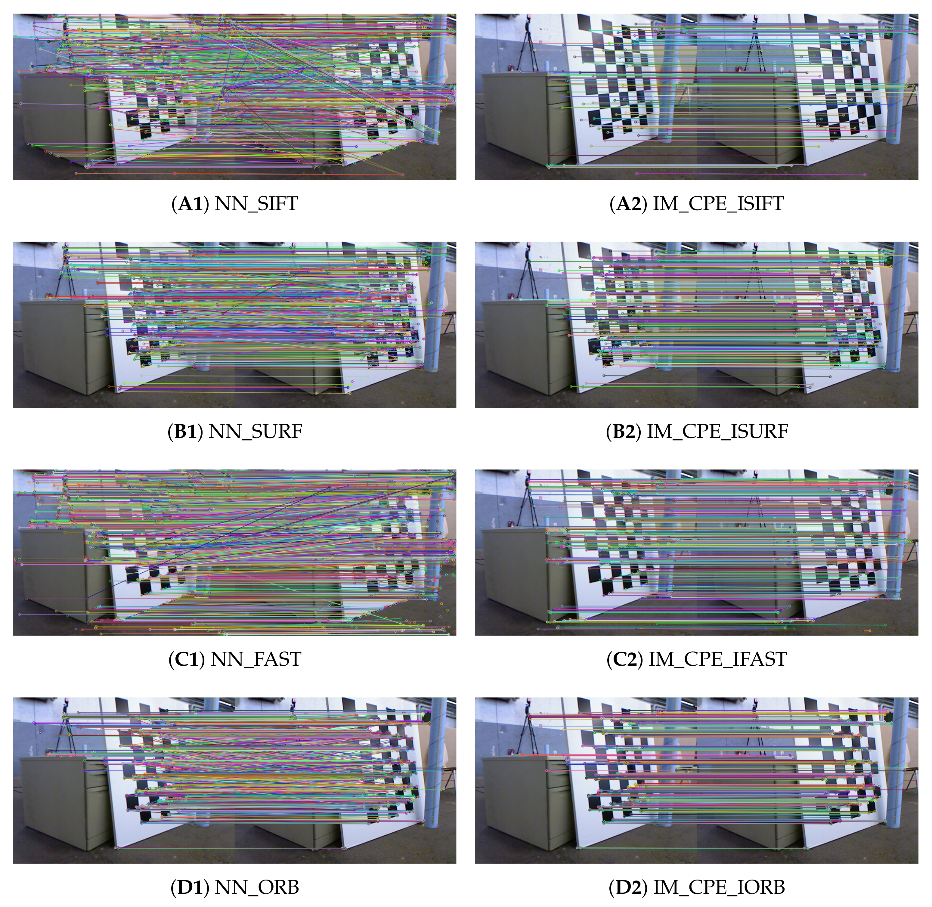
To demonstrate the superiority of IM_CPE, we compare the performance of the proposed method with existing work. As Figure 5 demonstrated, we conducted the experiments on IM_CPE and the nearest neighbor (NN) method using SIFT [3], SURF [4], ORB [8], and FAST [47]. It has to be mentioned that we apply a fixed threshold selection to obtain the putative good matches for the NN method for the four algorithms. For ORB [8], we extract 1500 key points in each image and for the NN method, and we assume that a match is good if the distance between the descriptors is less than the largest of twice the minimum distance of matched descriptors and the empirical value of 30. For SIFT [3] and SURF [4], we also extract 1500 key points and we select the top 50% matching key points with the smallest distance as the good matches. As for the FAST [47] key points, we also extract 1500 key points with SIFT [3] descriptors and the remaining steps are similar to SIFT [3].

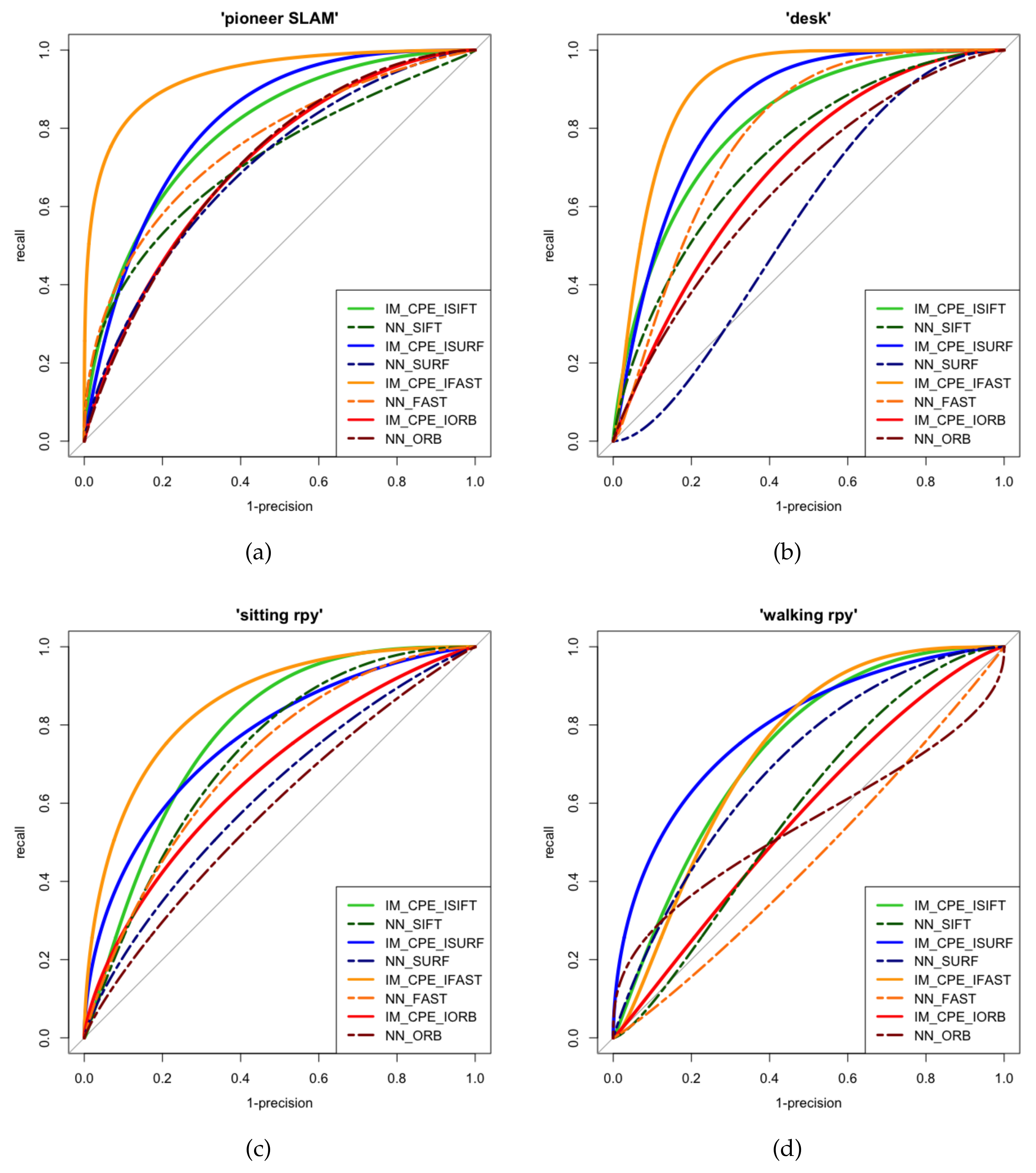
As we mentioned in Section 4.1, the performance of IM_CPE is better when $T_M\in [0.8,1.2]$. Thus, we chose $T_M=1$ for comparison. Figure 6 demonstrates the comparison of IM_CPE and the existing NN method using different key point methods in the four sequences in terms of recall v.s. 1-precision curve. It can be seen from Figure 6 that all the recalls of four key points extraction algorithms using IM_CPE were able to approach 1 faster than the NN method, especially SIFT [3], FAST [47], and SURF [4]. Although the result of IM_CPE using improved ORB is not obviously improved compared to other key points algorithms, it still performs better than using NN for matching even in the worst case.

The results of the NN_mAP and M.Score are demonstrated in

Table 5. Comparison of proposed IM_CPE and existing NN method using different key points extraction methods in terms of NN_mAP and M.Score.

	‘Pioneer SLAM’		‘Desk’		‘Sitting Rpy’		‘Walking Rpy’
	NN_mAP	M. Score	NN_mAP	M. Score	NN_mAP	M. Score	NN_mAP	M. Score
NN_SIFT [3]	0.716	0.274	0.548	0.075	0.726	0.189	0.580	0.078
IM_CPE_ISIFT	0.796	0.714	0.690	0.359	0.781	0.368	0.735	0.181
NN_SURF [4]	0.698	0.345	0.551	0.100	0.621	0.217	0.695	0.064
IM_CPE_ISURF	0.814	0.912	0.813	0.313	0.765	0.338	0.792	0.085
NN_FAST [47]	0.757	0.243	0.633	0.075	0.709	0.130	0.457	0.034
IM_CPE_IFAST	0.932	0.798	0.797	0.234	0.759	0.205	0.733	0.148
NN_ORB [8]	0.685	0.137	0.636	0.059	0.582	0.078	0.547	0.036
IM_CPE_IORB	0.709	0.373	0.702	0.167	0.670	0.164	0.790	0.048

and the best results are highlighted in bold. As can be seen, both the NN_mAP and M.Score of the proposed IM_CPE are higher than the traditional NN method in all sequences, which illustrates that IM_CPE is more superior compared to the NN method. For SIFT [3], SURF [4], and FAST [47], which use Euclidean distance to match descriptors, the performance of image matching has been improved significantly. When using ORB [8] and IM_CPE to match images, the improvement of the performance is not as significant as the others. However, relatively speaking, IM_CPE using ORB [8] is stable and obviously improved compared to the NN method, especially the M.Score, which has a steady increase in all four sequences, while the others only have a great improvement in M.Score in some sequences.

5. Discussions

Traditional image matching methods mainly match the local features through the distance of descriptor vectors on the full-size RGB images. However, in some cases, such as low image textures, structures, and large angular rotations, the distance between similar descriptors increases, and in some specific scenes may be so similar to each other that the descriptors cannot distinguish between them. As in the TUM RGBD dataset [46] we used the ‘pioneer SLAM’ sequence and ‘desk’ sequence contain some indoor scenes with high similarity and ‘sitting rpy’ and ‘walking rpy’ contain a dynamic object, all of these sequences will cause trouble when using the NN method for image matching, as Figure 5(A1,B1,C1,D1) demonstrated.

We proposed to generate and segment point cloud planes from the depth images and match these point cloud planes and then extract as well as match feature points on the matched planes. In this way, 2-D feature points will be extra constrained by the 3-D position and the matched point cloud plane in which it is located. Matching feature points on the matched plane reduces the number of feature points needed for a single matching task and effectively avoids matching a feature point with another one in an unrelated region, which is a common scenario in the NN method. However, matching on the matched plane decreases the probability of matching with feature points on another matched plane; still, it increases the probability of matching with feature points in the matched plane. Theoretically, the 3-D distance between a pair of perfectly matched feature points should be exactly equal to the distance between the centroid distance of two matched planes. Due to the discrete nature of the point cloud and the error in measuring the depth, the distance between the feature points and the distance between the centroid of the matched plane may introduce an error. Thus, we further propose to use the centroid distance controlled by a threshold to constrain the feature points in the matched plane. Therefore, we propose the IM_CPE to match feature points.

In general, IM_CPE can be well used to match various types of feature points and descriptors, including HOG descriptors and binary descriptors. The result of IM_CPE using ISIFT, ISURF, IFAST, and IORB has a significant improvement compared to the conventional NN method. More specifically, the NN_mAP performance of IM_CPE using IFAST on the four sequences has been improved by 16.63% on average, which is the highest compared to the values of 11.25% of ISIFT, 13.98% of ISURF, and 10.53% of IORB. Meanwhile, the M.Score performance of IM_CPE has been improved by 25.15% using ISIFT, 23.05% by using ISURF, 22.78% by using IFAST, and 11.05% by using IORB. Although it can be seen from Figure 6 that the performance and improvement of IM_CPE using ISIFT, ISURF, and IFAST are stronger than IORB, IM_CPE using IORB is better than the traditional NN method even in the worst case. Specifically, in the ‘pioneer SLAM’ sequence, the NN_mAP and M.Score are improved by 2.4% and 26.6%, respectively, and in the ‘walking rpy’ sequence the NN_mAP and M.Score are improved by 24.3% and 1.2%, respectively.

In summary, using IM_CPE to match descriptors works better than the traditional NN method, especially in HoG descriptors, which use Euclidean distance to measure the similarity of descriptors. The performance in binary descriptors matching is not as good as the HoG descriptors. We consider that the reason for such a discrepancy is that the distribution of feature points extracted by ORB [8] is relatively concentrated, so using the 3-D distance between feature points as an additional constraint is not enough to better distinguish the differences between the descriptors. In addition, the scale invariance of binary descriptors is not as good as HoG descriptors. Although the IM_CPE can help improve the scale invariance by measuring the relative position relationship, IM_CPE using improved ORB is not as satisfying as the others. However, the binary descriptors are faster than HoG descriptors and can be used in real time. Therefore, how to improve the matching result on such binary descriptors is the focus of our future work.

6. Conclusions

In this paper, a robust image matching method, IM_CPE, is proposed. We improve the performance of image matching by matching feature points on matched planes from the depth images instead of on full-size RGB images. The depth value and point cloud are used to simulate the real 3-D world. The point cloud planes are generated and segmented from depth images using the proposed PCPS algorithm and are then matched based on the centroid distance and the angle of the point cloud plane using the proposed PCPM algorithm. The KMAP algorithm is proposed to extract feature points from the input images based on the pair of matched point cloud planes and then the 2-D feature points are mapped into 3-D points. To match the feature points, we further propose the KMAT algorithm to match feature points based on the distance of their corresponding 3-D points and the distance between their descriptors. Simultaneously, by using the centroid distance to constrain the distance of the 3-D points, the robustness of the proposed KMAT algorithm is guaranteed. The proposed IM_CPE demonstrates excellent performance in image matching. The well-known key point extraction algorithms, SIFT [3], SURF [4], FAST [47], and ORB [8], are integrated and improved in our proposed IM_CPE, and the experimental results indicate the flexibility and superiority of the proposed method. Specifically, even in scenes with dynamic objects, our method demonstrates a strong matching performance. In summary, the proposed scheme shows robustness in image matching. Considering that the proposed method has little improvement in binary descriptors such as ORB [8], in our future work we will focus on improving the generality of the proposed matching method.