Article

An ADMM-qSPICE-Based Sparse DOA Estimation Method for MIMO Radar

1
School of Information and Communication Engineering, University of Electronic Science and Technology of China (UESTC), Chengdu 611731, China
2
Yangtze Delta Region Institute, University of Electronic Science and Technology of China (UESTC), Quzhou 324003, China
*
Author to whom correspondence should be addressed.
Remote Sens. 2023, 15(2), 446; https://doi.org/10.3390/rs15020446
Submission received: 20 November 2022 / Revised: 7 January 2023 / Accepted: 9 January 2023 / Published: 11 January 2023
(This article belongs to the Special Issue Theory and Applications of MIMO Radar)

Abstract

:
In recent years, sparse direction-of-arrival (DOA) estimation for multiple-input multiple-output (MIMO) radar has attracted extensive attention and been extensively studied, especially the method based on the classic least absolute shrinkage and selection operator (LASSO) estimator. The alternating-direction method of multipliers (ADMM) is an effective method for solving this problem at the cost of introducing an additional user parameter. To avoid introducing an additional user parameter, this paper adopts an equivalent transformation in the form of the generalized SParse Iterative Covariance-based Estimation (qSPICE) cost function to obtain a mean squared minimized form of the cost function. Then, the problem is transformed into a sparse optimization problem in the form of a weighted LASSO. Next, this unconstrained optimization problem is decomposed into three subproblems, which are solved separately to reduce the dimension of each problem and thus reduce the overall computational complexity based on ADMM. Simulation results and measured data indicate that the proposed method significantly outperforms the traditional super-resolution DOA estimation method and ADMM-LASSO method and slightly outperforms qSPICE in terms of resolution and sidelobe suppression capability. In addition, the proposed method has a much lower computational complexity and substantially fewer iterations than qSPICE.

Graphical Abstract

1. Introduction

In recent years, a new type of antenna system, multiple-input multiple-output (MIMO), has been introduced [1,2]. A MIMO antenna system is generally defined as a system that has multiple transmitted linearly independent waveforms and is capable of jointly processing multiple received antenna signals. MIMO radar draws on the idea of MIMO communication [3]. Its mechanism is to adopt transmit waveform diversity technology to improve the angular (spatial) resolution of the radar system while reducing the number of physical channels and antenna aperture, compared with traditional array antennas.
Estimation of the direction-of-arrival (DOA) of multiple targets in noise-polluted received data is the most important task in the practical application of centralized MIMO radar. The most fundamental DOA estimation method is the delay-and-sum (DAS) method, which can be implemented efficiently by fast Fourier transform (FFT) due to the Fourier structure of the orientation matrix. However, the resolution of this method is poor; to improve the positioning accuracy of the target source, many high-precision DOA estimation methods have been developed for traditional single-input multiple-output (SIMO) radar [4,5,6,7]. More recently, DOA estimation methods have been introduced into the field of centralized MIMO radar DOA estimation [8,9,10]. Among these methods, estimation of signal parameters via rotational invariance techniques (ESPRIT) and multiple signal classification (MUSIC) are relatively classic because of their simplicity and high-resolution performance [8,9]. Based on the orthogonality characteristics of the signal subspace and noise subspace, the multiple signal classification (MUSIC) method can lead to better DOA estimation performance than the DAS method with higher resolution. Taking advantage of the rotational invariance of the spatial correlation matrix signal subspace, the (ESPRIT) algorithm was proposed with excellent resolution and search-free advantages. In reference [10], the parallel factor analysis (PARAFAC) algorithm was proposed for a colocated MIMO radar with imperfect waveforms. ESPRIT is a low-dimensional and high-efficiency version of PARAFAC [11], and they have similar resolution performance. However, the resolution of these methods is limited, and noticeable performance degradation occurs when there are a few snapshots or a single snapshot. Recently, deep-learning techniques have been applied to DOA estimation for massive MIMO systems and achieved good system performance [12]. However, this method requires many training samples and the training phase is complex.
To further improve the resolution performance of MIMO radar DOA estimation, refs. [13,14] proposed the iterative adaptive method (IAA) for MIMO radar imaging; tests have demonstrated that the IAA method can function stably with a small number of snapshots or a single snapshot and has better angular resolution and target positioning accuracy. However, due to its high computational complexity, this method is difficult to apply in practical engineering [6]. Taking advantage of the sparsity of the source distribution, sparse learning via iterative minimization (SLIM) was proposed [15] for MIMO radar imaging. The method follows an L q -norm constraint and thus offers a more accurate estimate. In addition, SLIM has been demonstrated to have a higher angular resolution and lower computational complexity than IAA. Furthermore, a sparse spectrum estimation method with a higher resolution, called SParse Iterative Covariance-based Estimation (SPICE), was proposed based on weighted covariance fitting criteria [16,17]. This method is a semiparametric method, which converges globally and requires no selection of user parameters. In the case of a small number of snapshots, its frequency estimation performance is better than those of IAA and SLIM. However, the method has an L 1 -norm penalty (sparse constraint) for both signal and noise, which may result in a singular covariance matrix or many conditions. To avoid this problem, an improved algorithm, named qSPICE, was developed by introducing a L q -norm constraint on noise changes, where q 1 [18]. This method offers better estimation performance than SPICE. However, this method requires solving for the covariance matrix and its inverse, as well as performing the associated matrix multiplication operations to estimate each sampling grid point, which may result in a large computational burden, especially in massive MIMO (m-MIMO) signal processing.
With the increasing demand for higher reliability and higher data rates, novel MIMO antenna technologies are booming. In [19], an optimized algorithm based on semidefinite programming (SDP) and minimum mean squared error (MMSE) is proposed for s cognitive radio (CR) MIMO system. This method is proven to perform better in terms of total transmitted power and signal-to-interference plus noise ratio (SINR). To alleviate the large channel state information (CSI) feedback in m-MIMO system, a robust channel estimation scheme is proposed based on the separation mechanism of the channel matrix [20]. Moreover, some MIMO antenna design strategies and beamforming methods have also been well developed, such as m-MIMO antenna technology for 5G communication base stations [21,22], 10-element MIMO antenna design for new 5G smartphones [23,24], ultra-massive MIMO radar technology for terahertz antenna beamforming [25], etc. However, m-MIMO antenna arrangement requires the integration of a huge number of antennas at the base station and a large number of antennas at the user terminal, which will undoubtedly cause hardware implementation challenges and extremely high signal-processing complexity: whether it is for the spatial diversity and beamforming of MIMO communication systems [26], or directions of arrival (DOA) estimation of MIMO radar systems [17].
To reduce the high signal-processing complexity for m-MIMO systems, various advanced matrix inversion acceleration algorithms, such as the Neumann series (NS) algorithm [27] and the Jacobi algorithm [28], may be used to reduce the computational burden of qSPICE or IAA methods. In [29], the NS algorithm was used for matrix inversion approximation (MIA) for m-MIMO signal processing. This method transforms the matrix inverse problem into a matrix multiplication problem, which is suitable for hardware platforms, but its computational complexity is the same or even higher than those of direct inverse methods (e.g., QR-based methods [30]). Although the Jacobi method reduces the complexity from O N 3 to O L N 2 , where L represents the number of iterations, it converges slowly [31].
The alternating-direction method of multipliers (ADMM) is a powerful technique for solving massive optimization problems. This method is widely used in various fields, such as compressed sensing (CS) [32], regularization estimation [33], image processing [34], and machine learning [35]. In [36], the least absolute shrinkage and selection operator (LASSO)-ADMM algorithm was proposed for solving L 1 -norm constrained optimization problems for m-MIMO signal detection. In [37], ADMM was used to reduce the computational complexity of CS-DOA compared with the traditional interior point method (IPM); this method reduces the computational complexity by dividing the problem into multiple subproblems during the iteration process to reduce the dimension of each problem. In [38], an imprecise augmented Lagrange multiplier (ALM)-ADMM algorithm was proposed for solving a weighted mixed L 2 , 1 -norm penalty minimization problem to improve the DOA estimation performance for MIMO radar signals with missing elements.
Although the ADMM-based methods discussed above can efficiently solve the array DOA estimation problem, the application of an ADMM method introduces two additional user parameters, i.e., a Lagrangian parameter and a sparse regularization parameter [39]; the simultaneous adjustment of these two parameters is very tricky. To avoid this problem, in the present paper, the basic form of qSPICE is expanded, weighted covariance fitting is performed, and a mean square minimized form of the cost function is obtained by an equivalent transformation of the qSPICE cost function. Then, through the optimization properties, the problem is transformed into a sparse optimization problem in the form of a weighted LASSO. Then, this unconstrained optimization problem is decomposed into three subproblems to reduce the dimension of each problem and thus reduce the computational complexity based on ADMM. Due to the absence of user parameters in qSPICE, the proposed method can eliminate one sparse regularization parameter compared with the traditional ADMM-LASSO method, therefore significantly alleviating the difficulty of parameter selection. Meanwhile, the theoretical computational complexity of the proposed method is one order of magnitude lower than that of the traditional qSPICE method. Simulation results and measured data indicate that the estimation performance of the proposed method is not lower than those of qSPICE and ADMM-LASSO, and it incorporates the advantages of both methods, i.e., low complexity and a single user parameter.
The remainder of this paper is organized as follows. Section 2 reviews the MIMO radar signal model and the generalized SPICE and ADMM-LASSO methods. Then, the proposed ADMM-qSPICE DOA estimation method for MIMO radar is derived in detail. In Section 3, simulation and test results are presented, which demonstrate the effectiveness of the proposed method. In Section 4, the limitations of the proposed method are discussed. Section 5 presents the conclusions of this study.

2. Materials and Methods

2.1. MIMO Signal Model

We consider a centralized MIMO radar system equipped with M transmitting antennas and N receiving antennas. The transmitting and receiving antennas are assumed to be very close to each other such that the targets can be considered to be in the same orientation relative to them in the far field. It is assumed that the transmitting and receiving antennas of MIMO radar incorporate uniform linear arrays (ULAs) and that the MIMO radar system uses M transmitting antennas to transmit M mutually orthogonal waveforms with the same bandwidth and center frequency. Suppose there are K target sources. The DOA of the k-th target source is expressed as θ k k = 1 , 2 , , K . Based on the orthogonality of the transmitted signal waveform, the receiving array matches the filtered output; that is, the received data vector y t C M N × 1 can be expressed as [17,40,41]
y t = As t + e t
where s t = s 1 t , s 2 t , , s K t T C K × 1 represents the target source signal, in which s k t = α k · exp j ω k t , with  α k and ω k representing the reflection coefficient and Doppler angular frequency, respectively, of the k-th azimuth target; t denotes the distance-time variable; A = A t A r = a 1 , a 2 , , a K C M N × K is the orientation matrix; ⊙ represents the Khatri-Rao product; and e t denotes the covariance matrix of zero-mean white Gaussian noise σ 2 I M N , with  I M N denoting the M N × M N -dimensional unit matrix. A t and A r represent the transmitting and receiving orientation matrices, respectively, which can be expressed as
A t = a t θ 1 , a t θ 2 , , a t θ K C M × K
A r = a r θ 1 , a r θ 2 , , a r θ K C N × K
where a t θ k and a r θ k represent the transmitting and receiving orientation vectors, respectively, which are expressed as
a t θ k = 1 , exp j 2 π d t sin θ k / λ , , exp j 2 π d t M 1 sin θ k / λ T
a r θ k = 1 , exp j 2 π d r sin θ k / λ , , exp j 2 π d r N 1 sin θ k / λ T
where d t and d r represent the transmitting and receiving element spacings, respectively. The receiving element spacing is d r = λ / 2 , where λ represents the carrier wavelength. The transmitting element spacing is d t = M t · d r . According to MIMO theory, the equivalent virtual array of a MIMO system can be regarded as a SIMO ULA antenna with M N elements. Assuming there are L snapshots in total, the received data can be discretized as
y l = As l + e l
where s l C K × 1 is the target signal source to be estimated and e l C M N × 1 denotes noise, for  l = 1 , 2 , L . To simplify the model, it is assumed that the Doppler frequency of the target ω k = 0 ; at this point, the only target information to be estimated is the azimuth angle θ k and scattering intensity α k .
For many MIMO radar detection applications, such as airspace surveillance radar, the number of targets is considerably smaller than the number of potential source locations. In such a case, more accurate DOAs with higher resolution can be obtained using the sparsity of s . Below, two sparse signal recovery methods are considered, and the proposed method is derived in detail.

2.2. qSPICE

A classic sparse recovery method for solving model (6) is LASSO, whose cost function can be expressed as [42]
minimize s 1 2 y As 2 2 + μ s 1
where μ represents a user-adjustable regularization parameter, which balances the sparsity of the solution with the fitting degree of the signal. To avoid tricky parameter selection problems, an interesting alternative, namely the SPICE algorithm, was proposed in [16]. This method is based on the sparse covariance fitting criterion, and the minimization of the cost function can be expressed as
minimize p R 1 / 2 y y H R F 2
where
R = FP F H
F = A I M N = Δ a 1 , a 2 , , a M N + K
P = d i a g p
p = s 1 2 , s 2 2 , , s K 2 , σ 1 2 , σ 2 2 , , σ M N 2 = Δ p 1 , p 2 , , p K + M N
in which R 1 / 2 represents the Hermitian positive-definite root mean square of R 1 ; · F denotes the Frobenius matrix norm; · H is the conjugate transpose; d i a g · denotes a diagonal matrix composed of a specified vector; and σ i denotes the noise variance of MIMO channel i( i = 1 , 2 , , M N ). The minimization of (8) is equivalent to
minimize p k 0 y H R 1 y + Wp 1
where
W = d i a g w 1 , w 2 , , w K + M N
w j = a k 2 y 2 , j = 1 , 2 , , K + M N
The constraint of (13) is a weighted L 1 norm; this constraint tends to make its solution sparse. As expressed in (12), the SPICE algorithm simultaneously penalizes signal and noise. However, the penalty does not distinguish between signal and noise terms. Therefore, the minimized solution (13) will also cause the solution for the noise variance to tend to be sparse; that is, some values will be 0. In such a case, the covariance matrix R is not of full rank, which leads to two problems: unsatisfactory sparsity and an estimated increase in the model order [18]. To address these problems, a generalized SPICE algorithm, namely the qSPICE algorithm, was proposed based on the second constraint in the improved expression (13):
minimize p k 0 y H R 1 y + W s p s 1 + W n p n q
where
p s = p 1 , p 2 , , p K T
p n = p K + 1 , p K + 2 , , p K + M N T
W s = diag w 1 , w 2 , , w K
W n = diag w K + 1 , w K + 2 , , w K + M N
in which · q represents the vector q norm ( q > 0 ). The sparsity of the noise variance can be directly controlled by selecting a suitable value for q. When q = 1 , qSPICE degenerates into the classic SPICE algorithm. Therefore, the robustness of the estimation results can be improved by increasing the noise variance constraint term in Equation (16). However, the computational complexity of this method is too high, and it requires multiple matrix multiplication operations and one M N × M N matrix inversion operation in each iteration. Its computational complexity is O J K M N 2 + M N 3 , where J represents the number of iterations, which may generally be several hundred according to the authors’ experience [16]. Such high complexity is not conducive to practical engineering applications.

2.3. ADMM

There is also an effective divide-and-conquer approach for solving the optimization problem (7), namely the ADMM algorithm [43]. It has both the strong convergence characteristics of the multiplier method and the decomposability of the dual maximization problem. The LASSO problem is rewritten as a separable convex optimization problem with linear constraints (ADMM standard form) as follows:
minimize s , z 1 2 y As 2 2 + μ z 1
subject to
s = z
where z C K × 1 is an intermediate variable. The constrained optimization problem (21) is equivalent to the unconstrained optimization problem (22).
According to the multiplier method, the augmented Lagrangian function is constructed as
L ρ s , z , u = 1 2 y As 2 2 + μ z 1 + u T s z + ρ 2 s z 2 2
where u C K × 1 is an intermediate variable and ρ is an introduced penalty parameter related to the constraint condition that satisfies ρ > 0 . According to the ADMM algorithm [36], only one variable is updated at a time, while the other two variables are fixed, and the updating process is repeated alternately. For iterations j = 1 , 2 , , J , the following equations are applied:
s j + 1 = argmin s L ρ s , z j , u j z j + 1 = argmin z L ρ s j + 1 , z , u j u j + 1 = u + s j + 1 z j + 1
According to the equations above, each variable is updated successively through the following three steps:
s update:
s j + 1 = A T A + ρ I 1 A T y + ρ z j u j
z update:
z j + 1 = S o f t u j + s j + 1 , μ ρ
where S λ / ρ · is the soft threshold function, which satisfies
S o f t u j + s j + 1 , μ ρ = x μ ρ x > μ ρ 0 x μ ρ x + μ ρ x < μ ρ
u update:
u j + 1 = u j + s j + 1 z j + 1
According to our experience, the ADMM algorithm can lead to a satisfactory value of (25) after dozens of iterations by iteratively alternating among (25)–(28). Since the original problem is decomposed into three subproblems for solution, the variable dimension of each step of the alternating update is low, and the updating steps of z and u only involve vector addition and subtraction operations, resulting in low computational complexity. Notably, the computational complexity of this problem is mainly due to the calculation of the first matrix inverse in Equation (25). This matrix is constant in each iteration, so the matrix inverse must only be computed once in the algorithmic process. The computational complexity of this algorithm is O K 3 .
Compared with the qSPICE algorithm, this method has great advantages in terms of computational complexity, but it introduces a new user parameter, namely the Lagrangian parameter μ , on the basis of the sparse regularization parameter ρ of the original LASSO problem. Adjusting both μ and ρ at the same time is highly unpreferrable, which makes the method difficult to apply in practice.

2.4. Proposed Method

To avoid the above problem, we derive a new DOA estimation method with high resolution, high speed, and a single user parameter using the generalized SPICE problem model through the ADMM solution method.

2.4.1. ADMM-qSPICE

Similar to the derivation in [44,45], and assuming that the variances of the noise terms are consistent, i.e., i , σ i = σ , the optimization problem (16) can be equivalent to a weighted mean square LASSO problem [7,18]
minimize s y As 2 + Ds 1
where the weight matrix D satisfies
D = diag a 1 2 2 M N q · y 2 2 , a 2 2 2 M N q · y 2 2 , , a K 2 2 M N q · y 2 2
in which q is the control constraint parameter for noise in the generalized SPICE. We note that minimize s y As 2 + Ds 1 is a Lagrangian form of an optimization problem that is similar to minimize s y As 2 s . t . Ds 1 ε . This problem is equivalent to minimize s y As 2 2 s . t . D s 1 ε , where there is a bidirectional mapping relationship in D D [44]. In the simulation and processing of the measured data, we find that it is possible that D D , which can lead to excellent DOA results. Therefore, we solve the following weighted LASSO problem instead:
minimize s y As 2 2 + D s 1
We rewrite the above equation as
minimize s y As 2 2 + z 1
subject to
D s z = 0
and construct the augmented Lagrange function
L ˜ ρ s , z , u = 1 2 y As 2 2 + z 1 + u T D s z + ρ 2 D s z 2 2
According to the ADMM algorithm [36], only one variable is updated at a time, while the other two variables are fixed, and the update is repeated alternately. For iterations j = 1 , 2 , , J , we apply
s j + 1 = argmin s L ˜ ρ s , z j , u j z j + 1 = argmin z L ˜ ρ s j + 1 , z , u j u j + 1 = u j + ρ D s j + 1 z j + 1
According to the equations above, each variable can be updated successively through the following three steps: To simplify the form, we let ξ = u ρ and express (34) in scaled form:
L ˜ ρ s , z , ξ = 1 2 y As 2 2 + z 1 + ρ 2 D s z + ξ 2 2 ρ 2 ξ 2 2
s update:
Taking the derivative of (36) with respect to s and setting it to 0 yields
L ˜ ρ s = A T ( y As ) + ρ 2 · 2 · D T ( D s z + ξ ) = 0
Therefore, the iteration formula for the variable s can be written as
s j + 1 = ( A T A + ρ D T D ) 1 ( A T y + ρ D T ( z j ξ j ) )
z update:
Taking the derivative of (36) with respect to z yields
L ˜ ρ z = ( z 1 + ρ 2 D s z + ξ 2 2 ρ 2 ξ 2 2 ) z = ( ρ 2 z 1 + z ( D s + ξ ) 2 2 ) z
The solution to the above problem can be represented by the soft threshold [46] and expressed as
z j + 1 = S o f t ξ j + D s j + 1 , 1 ρ = ξ j + D s j + 1 + 1 ρ , ξ j + D s j + 1 > 1 ρ 0 , ξ j + D s j + 1 1 ρ ξ j + D s j + 1 1 ρ , ξ j + D s j + 1 < 1 ρ
u update:
The iterative formula for variable u can be written as
u j + 1 = u j + ρ ( D s j + 1 z j + 1 ) , u j = ρ ξ j
By alternating iteration of Equations (38)–(41), the DOA result s of the proposed method can be obtained. Algorithm 1 presents the pseudocode of this method. The matrix Δ and vectors Φ and c represent intermediate variables. The iteration termination criterion is s j + 1 s j ε , where ε is a small positive number. sign · represents the sign function, ⊙ denotes the Hadamard matrix product, and  max · denotes the maximum of two numbers.
Algorithm 1 ADMM-qSPICE
1:
D is initialized from (30), and  Δ = ( A T A + ρ D T D ) 1 is calculated. We set Φ = A T y , j = 1 , u = 0 , z = 0 , and  s = 0 .
2:
While the termination criterion is not satisfied, do
3:
       s j + 1 = Δ · Φ + ρ D T z j ξ j is updated.
4:
      We let c = ξ j + D s j + 1 .
5:
       z j + 1 = sign c max 0 , c 1 / ρ is updated.
6:
       u j + 1 = u j + ρ ( D s j + 1 z j + 1 ) is updated.
7:
       ξ j + 1 = u j + 1 / ρ is updated.
8:
      We set j = j + 1 .
9:
End while

2.4.2. Computational Complexity Analysis

As presented in Algorithm 1, the proposed ADMM-qSPICE method can be implemented by iterating (39)–(41) and performing some initialization calculations. We update s using Equation (38); because its left term is a fixed matrix in each iteration of the loop, it can be calculated beforehand for backup. Similarly, Φ is calculated in advance during initialization for backup, which can significantly reduce the computational complexity of the algorithm. The following is a complexity analysis of the initialization and iteration processes. In Step 1 of Algorithm 1, initializing D requires K + 2 M N multiplication operations. Calculating A T A requires M N 2 K multiplication operations. Since D is a diagonal matrix, calculating D T D only requires K multiplication operations, and inversion of the matrix K × K has a computational complexity of K 3 . Therefore, Δ is required to initialize M N 2 K + K 3 + K . Initializing Φ requires K M N multiplication operations. Thus, the computational complexity of the initialization portion is M N 2 K + K 3 + 2 K + 2 M N + K . In the iterative process of Algorithm 1, updating s requires 2 K 2 + K multiplication operations, while updating z requires K 2 + K multiplication operations. Updating u requires K 2 + 2 K multiplication operations. We suppose J iterations are required; then, the computational complexity of the iterative process is J 4 K 2 + 4 K . In summary, the complexity of the algorithm is K 3 + M N 2 K + 2 K M N + 4 J K 2 + 4 J + 1 K + 2 M N . The computational complexity of the iterative process of the proposed method is not high, and its main computational load corresponds to the initialization of Δ .
A comparison of the DAS method, IAA method, ADMM-LASSO method, qSPICE method and proposed method in terms of computational complexity is shown in Table 1, where J 1 J 4 represent the numbers of iterations for IAA, ADMM-LASSO, qSPICE and proposed method, respectively. Notably, the number of iterations J 1 for IAA is set to a fixed value of 12; J 2 , J 3 and J 4 depend on the termination criteria of the corresponding algorithms.

3. Results

In this section, the performance of the proposed ADMM-qSPICE method is demonstrated by simulation and testing. First, we conduct simulation tests to verify the DOA estimation accuracy and super-resolution ability of the proposed method. Then, we further evaluate the estimation accuracy and calculation time of the proposed method using two sets of measured data. The methods that are compared in this paper are DAS, IAA, ADMM-LASSO and qSPICE. Since only the angle estimation performance of each method is considered in this study, the target is set to be static and located at different azimuth angles of the same distance element. All our simulations and measurements are performed on a PC workstation equipped with 64-bit MATLAB R2018a, an Intel Core i5-9500 CPU (3.0 GHz) and 16 GB RAM. The root mean square error of angle estimation is used to evaluate the simulation performance of the proposed method, which is defined as
RMSE = 10 log 10 1 P p = 1 P θ ^ p θ p 2
where θ p represents the true value of the target angle of the p-th target grid and θ ^ p denotes the corresponding estimated value. The signal-to-noise ratio (SNR) is defined as
SNR = 10 log 10 P s δ 2
where P s represents the signal power and σ 2 is the variance of the additive white Gaussian noise.

3.1. Simulation Results

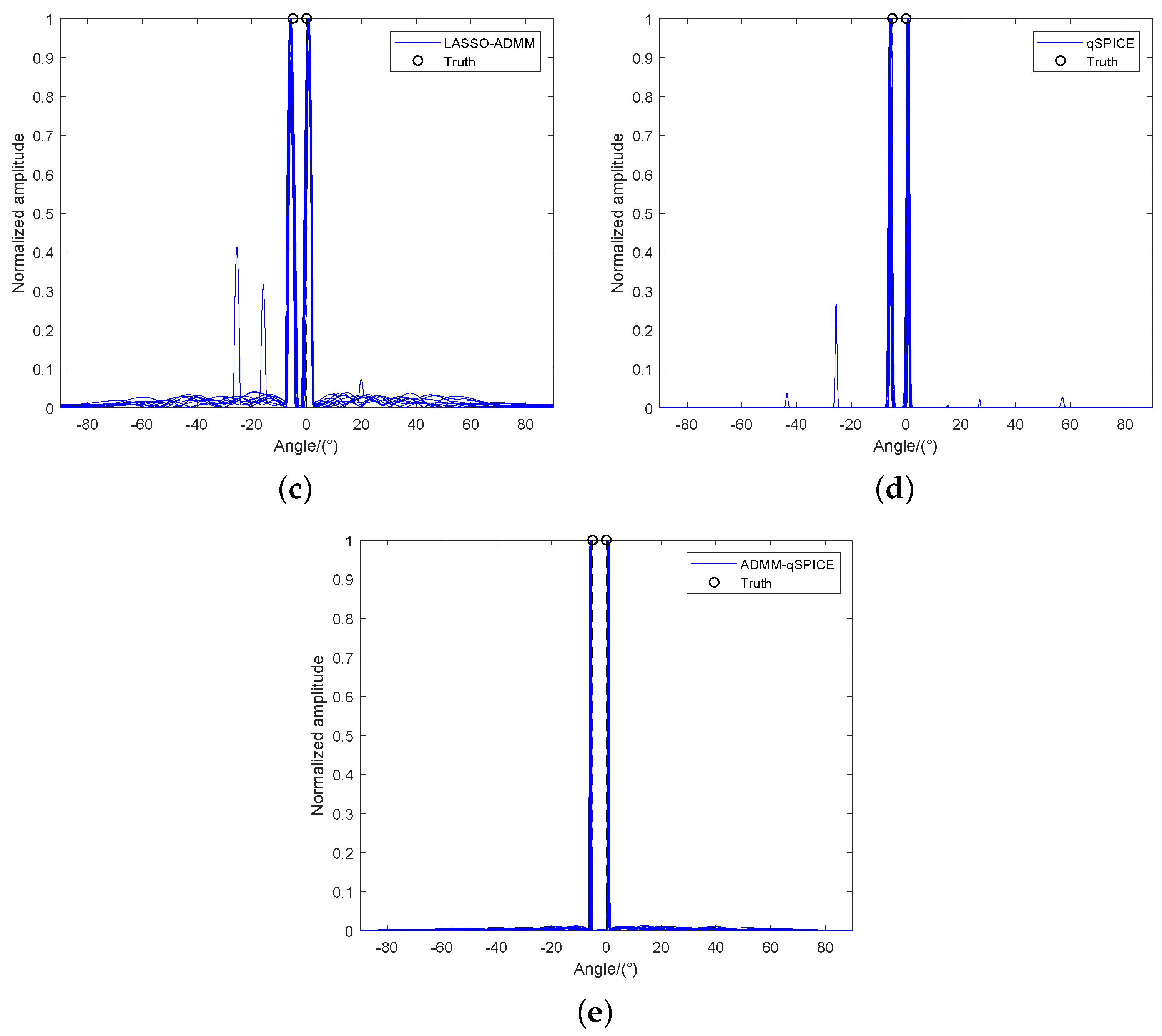
It is assumed that there are two independent sources with the same radiation power, which are located at azimuth 5 and 0 , respectively. The azimuth scanning range is 90 , 90 , and the number of target points is K = 512 . The SNR is set to SNR = 10 dB . We consider a 2-T 4-R MIMO radar system with a carrier frequency of f c = 77 GHz , a receiving element spacing of d r = λ / 2 = 1.9 mm , and a transmitting element spacing of d t = M t · d r = 7.6 mm .
Figure 1a shows the results of 10 Monte Carlo tests with the traditional DAS method. This method can be implemented quickly by FFT, but the azimuth resolution of the DOA results is very low, resulting in an inability to resolve two adjacent targets effectively. Figure 1b shows the results of 10 Monte Carlo tests with the IAA method. This method significantly outperforms the traditional DAS method in terms of sidelobe suppression, resolution and positioning accuracy, and the two targets are distinguished successfully in all 10 tests. However, this method still has various problems, i.e., unsatisfactory resolution, high sidelobes, and high computational complexity. Figure 1c shows the results of 10 Monte Carlo tests with the LASSO-ADMM method in [36], where the user parameters λ = 1 and ρ = 10 . We manually adjust these two parameters based on the quality of the DOA result. This quality specifically expressed as target resolution, 3 dB width, and DOA accuracy. The values of λ = 1 and ρ = 10 were obtained by extensive experiments and are the parameters that we believe are good for the ADMM-LASSO method under the simulation conditions in this paper. This method can distinguish the two adjacent targets well in most cases, and the sidelobe suppression effect is better than that of IAA. However, the method requires the adjustment of two user parameters at the same time in the process of implementation. When any of these parameters change, the target’s resolution, 3 dB width, and DOA accuracy decrease. Hence, this is a very tricky problem in engineering applications. Figure 1d shows the results of 10 Monte Carlo tests with the qSPICE method, where q = 1.5 . This method can better recover the amplitude and position information of the target, and the DOA result is more sparse than that in Figure 1c. However, the computational complexity of this method is quite high, especially for m-MIMO array problems. Figure 1e shows the results of 10 Monte Carlo tests with the proposed method, where q = 1.5 and ρ = 1.2 . The DOA results of the proposed method are better than those of DAS, IAA and LASSO-ADMM and are similar to those of qSPICE. In one of the Monte Carlo tests, qSPICE shows a spike with an amplitude of approximately 0.3 at 26 , but the proposed method only has a small peak with an amplitude of less than 0.05. The noise suppression ability of the proposed method clearly may be better than that of qSPICE when ρ = 1.2 is reasonably adjusted.
Figure 2 shows the root mean square error (RMSE) and Cramer-Rao bound (CRB) for the angle estimation results of the five methods over the SNR range of −5 dB to 30 dB. The RMSE of the proposed method is considerably lower than those of DAS and LASSO-ADMM, slightly lower than that of IAA, and similar to that of SPICE. In addition, as presented in Table 2, the target width of 3 dB when SNR = 10 dB quantitatively verifies the resolution performance of the proposed method. Moreover, the corresponding RMSE is presented. The proposed method clearly outperforms all the comparison methods above in terms of resolution, and its 3 dB width is the narrowest.

3.2. Measured Results

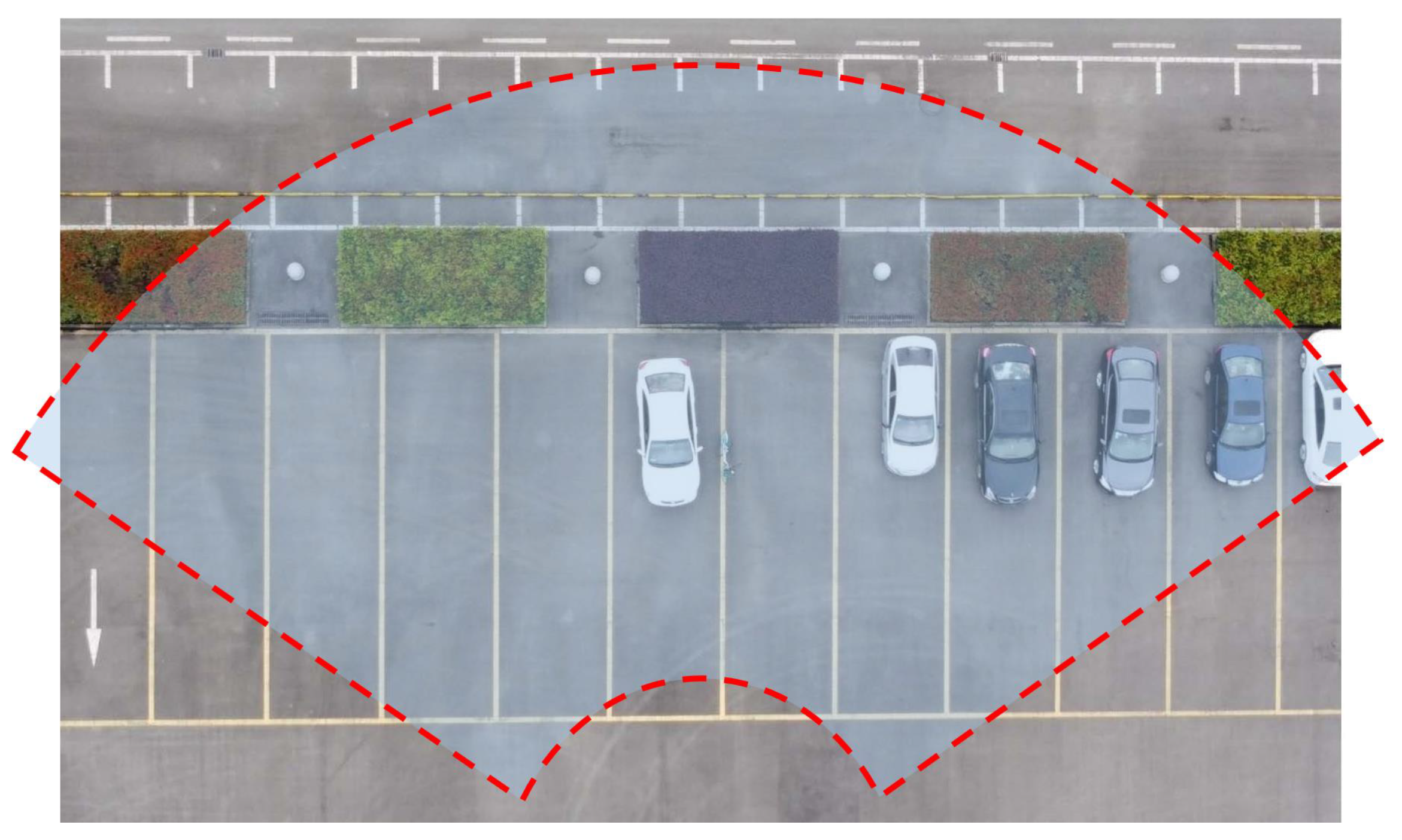
In this section, a set of MIMO radar measurements are used to verify the performance of the proposed method. An optical image of the original scene captured by an unmanned aerial vehicle (UAV) is shown in Figure 3, where the imaging area contains six vehicles. The MIMO radar parameters used in the test are shown in Table 3. There is a relationship among the carrier frequency, number of array elements and beam width, which jointly affect the azimuth resolution. The pulse width and pulse repetition interval affect the SNR. The bandwidth determines the range resolution.
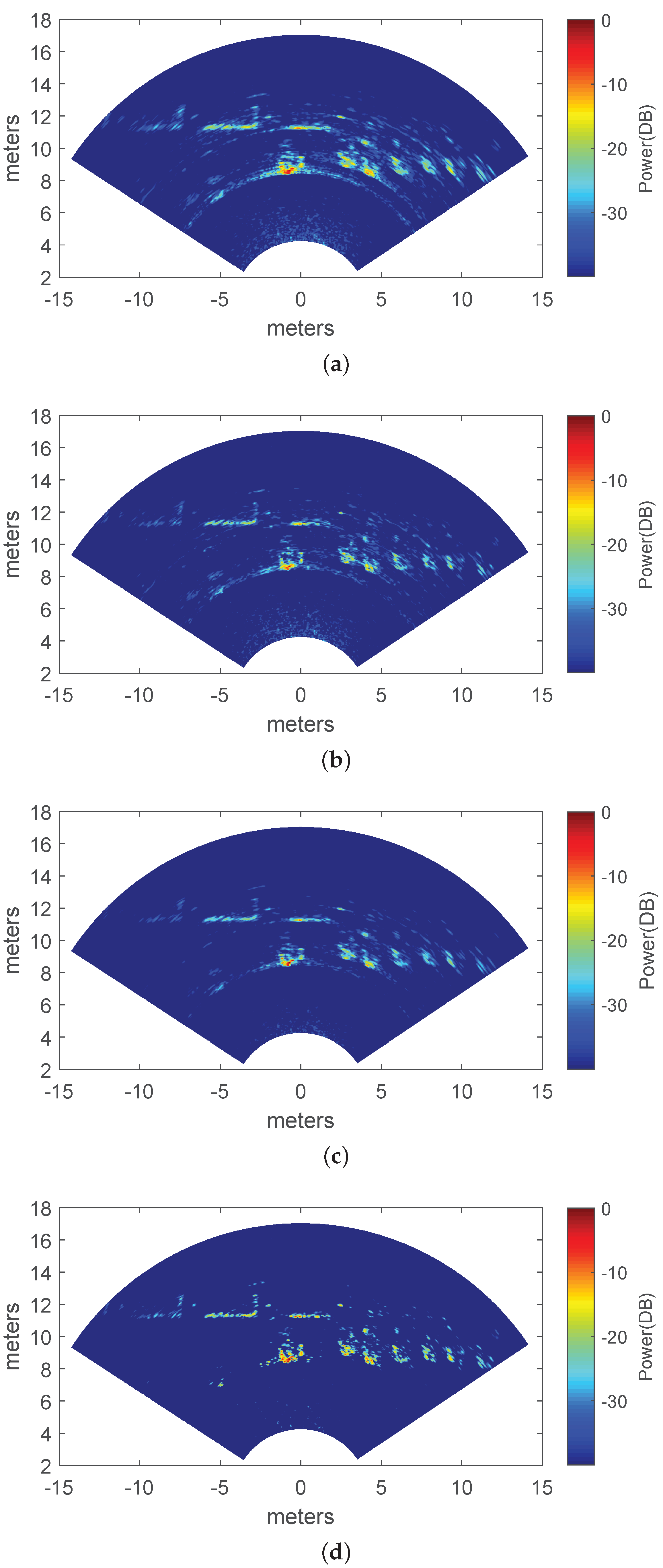
Figure 4a shows the two-dimensional results of the DAS method, with a processing time of 0.02 s. The echo energy of the middle car is strong; there is a clear front contour, but the sidelobe is quite high. The echo energies of the five vehicles on the right overlap and are blurred because DAS is based on traditional matching filtering, which suffers from low resolution and high sidelobes. Moreover, as can be seen from the Figure 4a, there are strip-shaped strongly scattered objects above the vehicles, which are actually caused by the stone edge of the flower bed. Figure 4b shows the two-dimensional results of the IAA method, for which the processing time is 115.13 s. The IAA method effectively improves the azimuth resolution of the image compared with DAS. The echo sidelobe of the middle car is significantly suppressed, and the vehicles in the dense group on the right can be better distinguished. Figure 4c shows the two-dimensional results of the ADMM-LASSO method, and its processing time is 2.40 s. This method can further improve the azimuth resolution of the target and better suppress the sidelobes compared with IAA. However, the method has two user parameters that must be adjusted, i.e., the sparse regularization parameter μ and Lagrangian parameter ρ . It is difficult to adjust both parameters at the same time in practical applications.
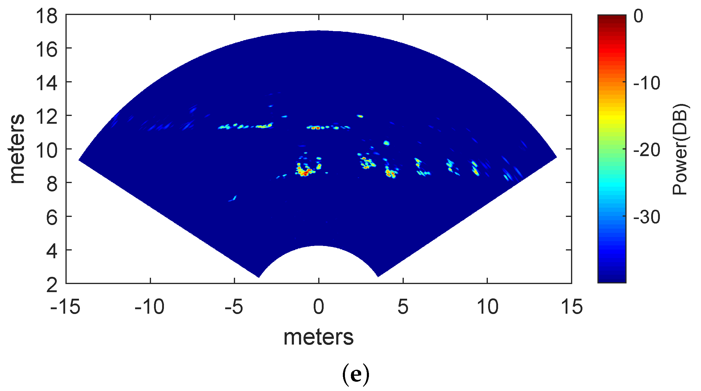
Figure 4d shows the two-dimensional results of the qSPICE method, with a processing time of 2704.81 s. As shown in the figure, this method further improves the azimuth resolution of the image compared with ADMM-LASSO. The sidelobes of the car in the center of the scene are significantly suppressed, and the car is more clearly defined. Unfortunately, the computational complexity of this method is too high, and the processing time is too long to be applied to real-time imaging applications with automotive radar, a consequence of the qSPICE method requiring high-dimensional matrix multiplication and inversion operations during the iteration process and requiring thousands of iterations per range element on average. Figure 4e shows the two-dimensional results of the ADMM-qSPICE method, with a processing time of 9.52 s. Compared with ADMM-LASSO, this method not only significantly improves the target resolution but also contains only one user parameter; thus, it is easier to apply in practice. Compared with the qSPICE method, the proposed method further suppresses the vehicle sidelobes. Sparser imaging results and more pronounced vehicle contours enable vehicles to be better detected and positioned. In addition, the computational complexity of this method is much lower than that of qSPICE method, because there is no need to calculate the matrix inverse in the iterations of the method, and the average number of iterations of each range element of the proposed method, i.e., 76, is considerably lower than that of the qSPICE method.
Image entropy (IE) was introduced to quantitatively analyze the two-dimensional target test results of the proposed method, where the lower the image entropy is, the better the image restoration effect [7]. The IE can be explicitly expressed by
IE = i = 1 I p i log 2 p i
where I denotes histogram counts of the two-dimensional image, and p i represents the probability of each gray level occurring. The image entropy of the processing results above is shown in Table 4 below. DAS clearly has the highest image entropy, which indicates poor image quality. The image entropy of IAA is lower than that of DAS, but the reduction is limited. ADMM-LASSO and qSPICE show significantly reduced image entropy compared with DAS and IAA, indicating that the image quality obtained by these two methods is better. As presented in the last row of Table 4, the image entropy of the proposed method is lower than those of other methods, which indicates that the proposed method has a stronger ability to suppress noise and sidelobes, therefore making the two-dimensional imaging performance on vehicles better and more conducive to vehicle detection and recognition.

4. Discussion

4.1. Results Analysis and Limitations

In this paper, an ADMM-qSPICE-based sparse DOA estimation method for MIMO radar was proposed. The proposed method was compared and verified in detail based on complexity analysis results, simulation results, and measured data for point and area targets. As shown in Figure 1 and Figure 4, the ADMM-qSPICE method achieved similar or even better resolution performance than traditional qSPICE. Moreover, the computational complexity of the ADMM-qSPICE method is considerably lower than that of the traditional qSPICE method. However, although the proposed method has the above two advantages, it also has various limitations.
As the ADMM algorithm was used to solve the problem, μ was introduced in the construction of the augmented Lagrangian function, which led to an additional user parameter that needed to be adjusted manually compared with the qSPICE method. Although one parameter is less complex than the two parameters of ADMM-LASSO, it is still difficult for practical applications. we always hope to obtain a user-parameter free method, which can adapt to different SNRs and sparsities. In follow-up efforts, we will study the variation rule of the Lagrangian parameter μ in different scenarios and seek an improved ADMM-SPICE method without user parameters.
Another limitation is that the computational complexity of the method is still large. Its computational complexity mainly comes from the matrix inversion in Equation (38). In the future work, we will further accelerate the calculation of high-dimensional matrix inversion for the proposed method.

4.2. Extended Applications

The proposed method can not only be used for the high accuracy DOA estimation of MIMO radar, but also can be applied to other radar imaging techniques, such as MIMO radar imaging, synthetic aperture radar (SAR) imaging [47] and real aperture radar (RAR) super-resolution imaging processing [6]. This is because, on the one hand, the signal models of the above problems are similar, and they can all be expressed as y = As + e . On the other hand, it is because the proposed method has good adaptability, few user parameters, low complexity, and easy implementation under various platforms.
In addition, the proposed method can also be employed to spatial diversity, beamforming, terminal locating and other techniques for m-MIMO antenna communication systems [48]. These techniques may apply to some equipment such as base stations with m-MIMO antennas and smartphones with new 5G MIMO antennas mentioned in [23,24].
For 5G communications and high accuracy MIMO radar, m-MIMO antenna systems are required to achieve high data rates and high angular resolution. Taking MIMO radar as an example, the higher the number of equivalent channels, the higher the angular resolution of the system, and the better the performance of the corresponding DOA estimation method. Therefore, theoretically, the proposed method can be applied to MIMO systems with infinite array elements. However, limited by the complexity of hardware implementation, the number of array elements in the actual MIMO radar is often limited. For the measured data of this paper, we use a 12 T × 16 R MIMO antenna system. We also made some simulations for m-MIMO antennas system. Due to the memory limitation of the simulation platform, the maximum number of MIMO elements in our simulation is 64 T × 64 R . The results show that the proposed method can still achieve good performance.

5. Conclusions

In this paper, a super-resolution DOA estimation method for MIMO radar based on ADMM-qSPICE was proposed. This approach has two significant advantages. First, compared with the ADMM-LASSO, the proposed method employs the weight matrix of the qSPICE to eliminate a user parameter and yield a higher resolution and stronger sidelobe suppression ability. Second, compared with qSPICE, the computational complexity of the proposed method is reduced from O J 3 M N 3 to O K 3 without performance loss. Furthermore, the proposed method can also be applied to MIMO radar imaging, SAR imaging and massive MIMO systems in 5G communication. In future work, we will further improve the proposed method to achieve completely parameter adaptation.

Author Contributions

Conceptualization, Y.Z. (Yongwei Zhang) and Y.Z. (Yongchao Zhang); methodology, Y.Z. (Yongwei Zhang); software, J.L.; validation, Y.Z. (Yongchao Zhang) and Y.Z. (Yongwei Zhang); formal analysis, Y.Z. (Yongwei Zhang); investigation, Y.Z. (Yongwei Zhang) and J.Y. (Jianan Yan); resources, Y.Z. (Yongwei Zhang); data curation, Y.Z. (Yongwei Zhang); writing—original draft preparation, Y.Z. (Yongwei Zhang); writing—review and editing, J.Y. (Jianan Yan); visualization, Y.Z. (Yongchao Zhang); supervision, Y.Z. (Yongchao Zhang); project administration, Y.Z. (Yongchao Zhang); funding acquisition, Y.Z. (Yongchao Zhang), Y.Z. (Yin Zhang), Y.H. and J.Y. (Jianyu Yang). All authors have read and agreed to the published version of the manuscript.

Funding

This work was supported in part by the National Natural Science Foundation of China under grants 61901092, 61901090, and was supported by the Municipal Government of Quzhou under Grant Number 2022D011 and 2022D036.

Data Availability Statement

This study did not report any data.

Conflicts of Interest

The authors declare no conflict of interest.

Abbreviations

The following abbreviations are used in this manuscript:
DOAdirections of arrival
MIMOmultiple-input multiple-output
LASSOleast absolute shrinkage and selection operator
ADMMalternating-direction method of multipliers
qSPICEgeneralized SParse Iterative Covariance-based Estimation
DASdelay-and-sum
FFTfast Fourier transform
SIMOsingle-input multiple-output
ESPRITestimation of signal parameters via rotational invariance techniques
MUSICmultiple signal classification
PARAFACparallel factor analysis
MVDRMinimum variance distortionless response
IAAiterative adaptive method
SLIMsparse learning via iterative minimization
SPICEsparse Iterative Covariance-based Estimation
NSNeumann series
MIAmatrix inversion approximation
CScompressed sensing
IPMinterior point method
ALMaugmented Lagrange multiplier
ULAuniform linear array
RMSEroot mean square error
CRBCramer-Rao bound
UAVunmanned aerial vehicle
SNRsignal-to-noise ratio
IEImage entropy

References

  1. Sharma, P.; Tiwari, R.N.; Singh, P.; Kumar, P.; Kanaujia, B.K. MIMO Antennas: Design Approaches, Techniques and Applications. Sensors 2022, 22, 7813. [Google Scholar] [CrossRef] [PubMed]
  2. Hu, X.; Tong, N.; Wang, J.; Ding, S.; Zhao, X. Matrix completion-based MIMO radar imaging with sparse planar array. Signal Process. 2017, 131, 49–57. [Google Scholar] [CrossRef]
  3. Fishler, E.; Haimovich, A.; Blum, R.; Chizhik, D.; Cimini, L.; Valenzuela, R. MIMO radar: An idea whose time has come. In Proceedings of the 2004 IEEE Radar Conference (IEEE Cat. No. 04CH37509), Philadelphia, PA, USA, 29 April 2004; pp. 71–78. [Google Scholar]
  4. Dai, J.; So, H.C. Real-valued sparse Bayesian learning for DOA estimation with arbitrary linear arrays. IEEE Trans. Signal Process. 2021, 69, 4977–4990. [Google Scholar] [CrossRef]
  5. Liang, Y.; Liu, W.; Shen, Q.; Cui, W.; Wu, S. A review of closed-form Cramér-Rao bounds for DOA estimation in the presence of Gaussian noise under a unified framework. IEEE Access 2020, 8, 175101–175124. [Google Scholar] [CrossRef]
  6. Zhang, Y.; Luo, J.; Zhang, Y.; Huang, Y.; Cai, X.; Yang, J.; Mao, D.; Li, J.; Tuo, X.; Zhang, Y. Resolution Enhancement for Large-Scale Real Beam Mapping Based on Adaptive Low-Rank Approximation. IEEE Trans. Geosci. Remote Sens. 2022, 60, 5116921. [Google Scholar] [CrossRef]
  7. Zhang, Y.; Luo, J.; Li, J.; Mao, D.; Zhang, Y.; Huang, Y.; Yang, J. Fast inverse-scattering reconstruction for airborne high-squint radar imagery based on Doppler centroid compensation. IEEE Trans. Geosci. Remote Sens. 2021, 60, 5205517. [Google Scholar] [CrossRef]
  8. Qiu, S.; Ma, X.; Zhang, R.; Han, Y.; Sheng, W. A dual-resolution unitary ESPRIT method for DOA estimation based on sparse co-prime MIMO radar. Signal Process. 2023, 202, 108753. [Google Scholar] [CrossRef]
  9. Meng, F.X.; Li, Z.T.; Xu-Tao, Y.; Zhang, Z.C. Quantum algorithm for MUSIC-based DOA estimation in hybrid MIMO systems. Quantum Sci. Technol. 2022, 7, 025002. [Google Scholar] [CrossRef]
  10. Ruan, N.J.; Wen, F.q.; Ai, L.; Xie, K. A PARAFAC decomposition algorithm for DOA estimation in colocated MIMO radar with imperfect waveforms. IEEE Access 2019, 7, 14680–14688. [Google Scholar] [CrossRef]
  11. Hassanien, A.; Vorobyov, S.A. Transmit energy focusing for DOA estimation in MIMO radar with colocated antennas. IEEE Trans. Signal Process. 2011, 59, 2669–2682. [Google Scholar] [CrossRef]
  12. Huang, H.; Yang, J.; Huang, H.; Song, Y.; Gui, G. Deep learning for super-resolution channel estimation and DOA estimation based massive MIMO system. IEEE Trans. Veh. Technol. 2018, 67, 8549–8560. [Google Scholar] [CrossRef]
  13. Roberts, W.; Stoica, P.; Li, J.; Yardibi, T.; Sadjadi, F.A. Iterative adaptive approaches to MIMO radar imaging. IEEE J. Sel. Top. Signal Process. 2010, 4, 5–20. [Google Scholar] [CrossRef]
  14. Shang, X.; Liu, J.; Li, J. Multiple object localization and vital sign monitoring using IR-UWB MIMO radar. IEEE Trans. Aerosp. Electron. Syst. 2020, 56, 4437–4450. [Google Scholar] [CrossRef]
  15. Tan, X.; Roberts, W.; Li, J.; Stoica, P. Sparse learning via iterative minimization with application to MIMO radar imaging. IEEE Trans. Signal Process. 2010, 59, 1088–1101. [Google Scholar] [CrossRef]
  16. Stoica, P.; Babu, P.; Li, J. New method of sparse parameter estimation in separable models and its use for spectral analysis of irregularly sampled data. IEEE Trans. Signal Process. 2010, 59, 35–47. [Google Scholar] [CrossRef]
  17. Luo, J.; Zhang, Y.; Yang, J.; Zhang, D.; Zhang, Y.; Zhang, Y.; Huang, Y.; Jakobsson, A. Online Sparse DOA Estimation Based on Sub–Aperture Recursive LASSO for TDM–MIMO Radar. Remote Sens. 2022, 14, 2133. [Google Scholar] [CrossRef]
  18. Swärd, J.; Adalbjörnsson, S.I.; Jakobsson, A. Generalized sparse covariance-based estimation. Signal Process. 2018, 143, 311–319. [Google Scholar] [CrossRef] [Green Version]
  19. Khan, I.; Al-Wesabi, F.N.; Obayya, M.; Hilal, A.M.; Hamza, M.A.; Rizwanullah, M.; Al-Zahrani, F.A.; Amano, H.; Mostafa, S.M. An Optimized Algorithm for CR-MIMO Wireless Networks. CMC Comput. Mater. Contin. 2022, 71, 697–715. [Google Scholar]
  20. Khan, I.; Rodrigues, J.J.; Al-Muhtadi, J.; Khattak, M.I.; Khan, Y.; Altaf, F.; Mirjavadi, S.S.; Choi, B.J. A robust channel estimation scheme for 5G massive MIMO systems. Wirel. Commun. Mob. Comput. 2019, 2019, 3469413. [Google Scholar] [CrossRef] [Green Version]
  21. Karad, K.V.; Hendre, V.S. Review of Antenna Array for 5G Technology Using mmWave Massive MIMO. In Recent Trends in Electronics and Communication; Springer: Singapore, 2022; pp. 775–787. [Google Scholar]
  22. Al-Tarifi, M.A.; Sharawi, M.S.; Shamim, A. Massive MIMO antenna system for 5G base stations with directive ports and switched beamsteering capabilities. IET Microwaves Antennas Propag. 2018, 12, 1709–1718. [Google Scholar] [CrossRef] [Green Version]
  23. Alja’Afreh, S.S.; Altarawneh, B.; Alshamaileh, M.H.; E’qab, R.A.; Hussain, R.; Sharawi, M.S.; Xing, L.; Xu, Q. Ten antenna array using a small footprint capacitive-coupled-shorted loop antenna for 3.5 GHz 5G smartphone applications. IEEE Access 2021, 9, 33796–33810. [Google Scholar] [CrossRef]
  24. Jaglan, N.; Gupta, S.D.; Kanaujia, B.K.; Sharawi, M.S. 10 element sub-6-GHz multi-band double-T based MIMO antenna system for 5G smartphones. IEEE Access 2021, 9, 118662–118672. [Google Scholar] [CrossRef]
  25. Elbir, A.M.; Mishra, K.V.; Chatzinotas, S. Terahertz-band joint ultra-massive MIMO radar-communications: Model-based and model-free hybrid beamforming. IEEE J. Sel. Top. Signal Process. 2021, 15, 1468–1483. [Google Scholar] [CrossRef]
  26. Li, X.; Wang, B. Coherence optimised subarray partition for hybrid MIMO phased array radar. IET Microwaves Antennas Propag. 2021, 15, 1441–1457. [Google Scholar] [CrossRef]
  27. Zhu, D.; Li, B.; Liang, P. On the matrix inversion approximation based on Neumann series in massive MIMO systems. In Proceedings of the 2015 IEEE International Conference on Communications (ICC), London, UK, 8–12 June 2015; pp. 1763–1769. [Google Scholar]
  28. Albreem, M.A. Approximate matrix inversion methods for massive mimo detectors. In Proceedings of the 2019 IEEE 23rd International Symposium on Consumer Technologies (ISCT), Ancona, Italy, 19–21 June 2019; pp. 87–92. [Google Scholar]
  29. Zhang, X.; Zeng, H.; Ji, B.; Zhang, G. Low Complexity Implicit Detection for Massive MIMO Using Neumann Series. IEEE Trans. Veh. Technol. 2022, 71, 9044–9049. [Google Scholar] [CrossRef]
  30. Prabhu, H.; Rodrigues, J.; Edfors, O.; Rusek, F. Approximative matrix inverse computations for very-large MIMO and applications to linear pre-coding systems. In Proceedings of the 2013 IEEE Wireless Communications and Networking Conference (WCNC), Shanghai, China, 7–10 April 2013; pp. 2710–2715. [Google Scholar]
  31. Song, W.; Chen, X.; Wang, L.; Lu, X. Joint conjugate gradient and Jacobi iteration based low complexity precoding for massive MIMO systems. In Proceedings of the 2016 IEEE/CIC International Conference on Communications in China (ICCC), Chengdu, China, 27–29 July 2016; pp. 1–5. [Google Scholar]
  32. Kouni, V.; Paraskevopoulos, G.; Rauhut, H.; Alexandropoulos, G.C. ADMM-DAD net: A deep unfolding network for analysis compressed sensing. In Proceedings of the ICASSP 2022—2022 IEEE International Conference on Acoustics, Speech and Signal Processing (ICASSP), Singapore, 23–27 May 2022; pp. 1506–1510. [Google Scholar]
  33. Qu, W.; Xiu, X.; Zhang, H.; Fan, J. An efficient semi-proximal ADMM algorithm for low-rank and sparse regularized matrix minimization problems with real-world applications. J. Comput. Appl. Math. 2022, 424, 115007. [Google Scholar] [CrossRef]
  34. Li, X.; Bai, X.; Zhou, F. High-resolution ISAR imaging and autofocusing via 2d-ADMM-net. Remote Sens. 2021, 13, 2326. [Google Scholar] [CrossRef]
  35. Shang, F.; Xu, T.; Liu, Y.; Liu, H.; Shen, L.; Gong, M. Differentially private ADMM algorithms for machine learning. IEEE Trans. Inf. Forensics Secur. 2021, 16, 4733–4745. [Google Scholar] [CrossRef]
  36. Elgabli, A.; Elghariani, A.; Al-Abbasi, A.O.; Bell, M. Two-stage LASSO ADMM signal detection algorithm for large scale MIMO. In Proceedings of the 2017 51st Asilomar Conference on Signals, Systems, and Computers, Pacific Grove, CA, USA, 29 October–1 November 2017; pp. 1660–1664. [Google Scholar]
  37. Wang, Q.; Zhao, Z.; Chen, Z. Fast compressive sensing DOA estimation via ADMM solver. In Proceedings of the 2017 IEEE International Conference on Information and Automation (ICIA), Macao, China, 18–20 July 2017; pp. 53–57. [Google Scholar]
  38. Chen, J.; Zhang, C.; Fu, S.; Li, J. Robust Reweighted 2,1-Norm Based Approach for DOA Estimation in MIMO Radar Under Array Sensor Failures. IEEE Sens. J. 2021, 21, 27858–27867. [Google Scholar] [CrossRef]
  39. Hashempour, H.R. Sparsity-driven ISAR imaging based on two-dimensional ADMM. IEEE Sens. J. 2020, 20, 13349–13356. [Google Scholar] [CrossRef]
  40. Li, J.; Stoica, P. MIMO Radar Signal Processing; John Wiley & Sons: Hoboken, NJ, USA, 2008. [Google Scholar]
  41. Wang, X.; Wang, L.; Li, X.; Bi, G. Nuclear norm minimization framework for DOA estimation in MIMO radar. Signal Process. 2017, 135, 147–152. [Google Scholar] [CrossRef]
  42. Tibshirani, R. Regression shrinkage and selection via the lasso. J. R. Stat. Soc. Ser. B 1996, 58, 267–288. [Google Scholar] [CrossRef]
  43. Boyd, S.; Parikh, N.; Chu, E.; Peleato, B.; Eckstein, J. Distributed optimization and statistical learning via the alternating direction method of multipliers. Found. Trends® Mach. Learn. 2011, 3, 1–122. [Google Scholar]
  44. Rojas, C.R.; Katselis, D.; Hjalmarsson, H. A note on the SPICE method. IEEE Trans. Signal Process. 2013, 61, 4545–4551. [Google Scholar] [CrossRef] [Green Version]
  45. Stoica, P.; Zachariah, D.; Li, J. Weighted SPICE: A unifying approach for hyperparameter-free sparse estimation. Digit. Signal Process. 2014, 33, 1–12. [Google Scholar] [CrossRef] [Green Version]
  46. Wright, S.J.; Nowak, R.D.; Figueiredo, M.A. Sparse reconstruction by separable approximation. IEEE Trans. Signal Process. 2009, 57, 2479–2493. [Google Scholar] [CrossRef] [Green Version]
  47. Yang, X.; Zhang, Y.; Mao, D.; Bu, Y.; Yang, H.; Shi, J. Sparse Reconstruction for Synthetic Aperture Radar VIA Generalized Sparse Covariance Fitting. In Proceedings of the IGARSS 2019—2019 IEEE International Geoscience and Remote Sensing Symposium, Yokohama, Japan, 28 July–2 August 2019; pp. 767–770. [Google Scholar]
  48. Ali, E.; Ismail, M.; Nordin, R.; Abdulah, N.F. Beamforming techniques for massive MIMO systems in 5G: Overview, classification, and trends for future research. Front. Inf. Technol. Electron. Eng. 2017, 18, 753–772. [Google Scholar] [CrossRef]
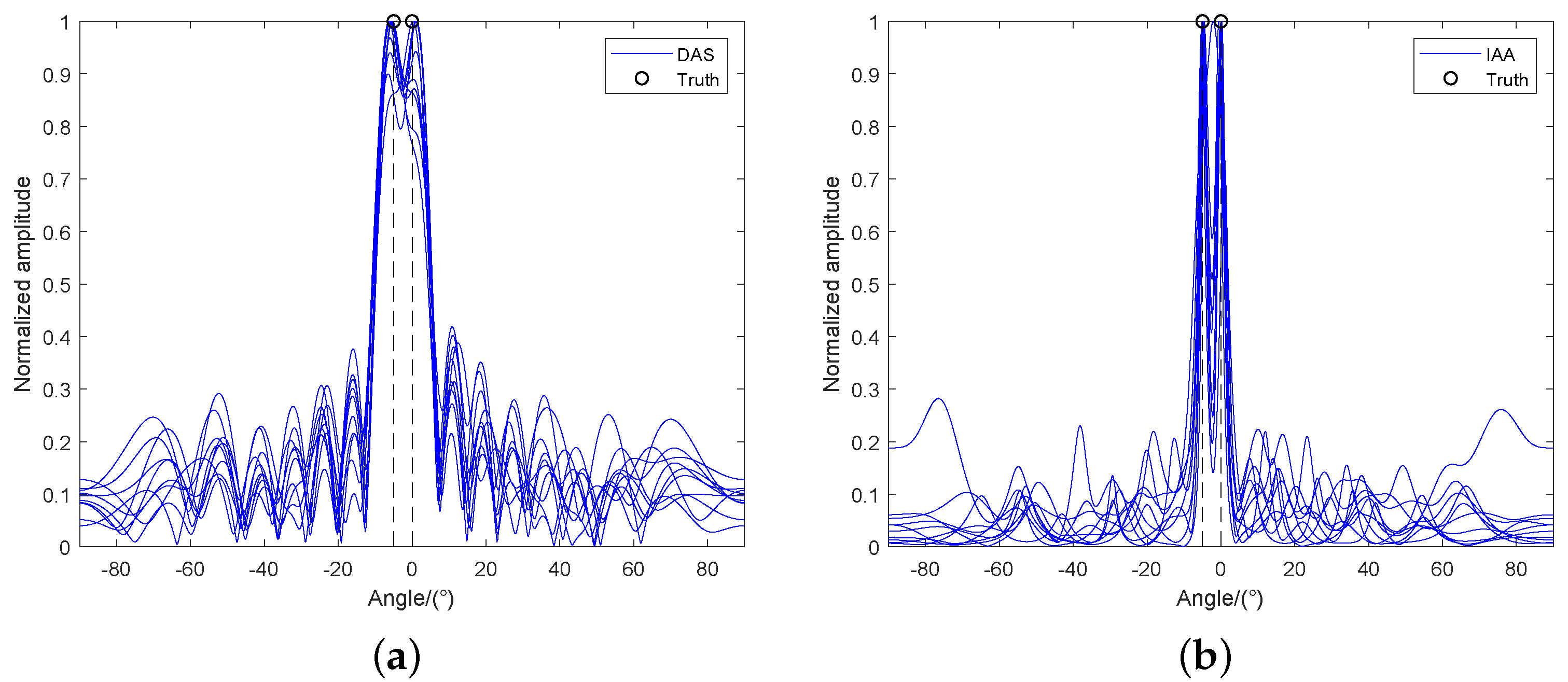
Figure 1. Simulated DOA results. (a) DAS method, (b) IAA method, (c) ADMM−LASSO method ( λ = 1 and ρ = 10 ), (d) qSPICE method, and (e) proposed method ( ρ = 1.2 ).
Remotesensing 15 00446 g001aRemotesensing 15 00446 g001b
Figure 2. RMSE and CRB of each method.
Remotesensing 15 00446 g002
Figure 3. Optical scene.
Remotesensing 15 00446 g003
Figure 4. Measured Data. (a) Two−dimensional result of the DAS method, (b) Two−dimensional results of the IAA method, (c) Two−dimensional results of the ADMM−LASSO method, (d) Two−dimensional results of the qSPICE method, and (e) Two−dimensional results of the ADMM−SPICE method.
Remotesensing 15 00446 g004aRemotesensing 15 00446 g004b
Table 1. Complexity comparison.
MethodNumber of Multiplication and Division OperationsComputational ComplexityComputational Time ( M N = 512 , K = 256 )
DAS (FFT) K log 2 K O K log 2 K 4.43 × 10 4 s
IAA [13] J 1 M N 3 + 2 M N 2 K + M N K O J 1 M N 3 4.88 s
ADMM-LASSO [36] K 3 + M N + J 2 K 2 + K M N O K 3 0.03 s
qSPICE [18] J 3 M N 3 + K + 1 M N 2 + K 2 + K + 1 M N + 12 K O J 3 M N 3 11.41 s
Proposed method K 3 + M N 2 K + 2 K M N + 4 J 4 K 2 + 4 J 4 + 1 K + 2 M N O K 3 0.13 s
Table 2. Performance Comparison of Various Methods (SNR = 10 dB).
Method3 dB Width (Degrees)RMSE (dB)
DAS16.8012.79
IAA2.260.15
ADMM-LASSO3.223.791
qSPICE1.32−2.269
ADMM-SPICE0.98−1.791
Table 3. Parameters of the Measured Data.
ParameterValue
Carrier frequency77 GHz
Bandwidth3.75 GHz
Beam width1.4
Pulse width1 ms
Pulse recurrence interval512 μ s
Number of transmitting array elements12
Number of receiving array elements16
Range sampling points261
Table 4. Image Entropy.
MethodsIE
DAS4.03
IAA3.70
ADMM-LASSO1.55
qSPICE1.08
ADMM-SPICE0.97
Disclaimer/Publisher’s Note: The statements, opinions and data contained in all publications are solely those of the individual author(s) and contributor(s) and not of MDPI and/or the editor(s). MDPI and/or the editor(s) disclaim responsibility for any injury to people or property resulting from any ideas, methods, instructions or products referred to in the content.