Abstract
HY-1C/D both carry a coastal zone imager (CZI) with a spatial resolution of 50 m and a swath width of 950 km, two observations can be achieved in three days when two satellites operating in a network. Accurate atmospheric correction is the basis for quantitative inversion of ocean color parameters using CZI However, atmospheric correction in estuarine and coastal waters with complex optical properties is a challenge due to the band setting of CZI. This paper proposed a novel atmospheric correction algorithm for CZI images applicable to turbid waters in estuarine and coastal zone. The Rayleigh scattering reflectance of CZI was calculated based on a vector radiative transfer model. Next, a semi-empirical radiative transfer model with suspended particle concentration as the parameter is used to model the water-atmosphere coupling. Finally, the parameters of the coupling model are solved by combining a global optimization method based on a genetic algorithm. The results indicate that the CZI-derived remote-sensing reflectance (Rrs) are in good agreement with the quasi-synchronous Landsat-8/9 operational land imager (OLI) derived Rrs in the green and red bands (R2 > 0.96). Validation using in situ data revealed that the RMSE of the CZI-derived Rrs in the green and red bands was 0.0036 sr−1 and 0.0035 sr−1. More importantly, the values and spatial distributions of suspended particulate matter (SPM) estimated by CZI and those estimated by OLI in the Subei Shoal and the Yangtze River Estuary are basically consistent, and the validation using in situ data revealed that the inversion of SPM concentration by CZI was effective (R2 = 0.86, RMSE = 0.0362 g/L), indicating that CZI has great potential and broad application prospects for monitoring the spatial and temporal dynamics of SPM in estuarine and coastal waters. The study results will lay the foundation for further estimating suspended sediment fluxes and carbon fluxes, thus providing data support and scientific basis for promoting resource development, utilization and conservation strategies in estuarine and coastal areas.
1. Introduction
The estuary is the hub of the basin and the ocean, and the coastal zone is the link between the land and the ocean. Estuarine and coastal areas are the concentrated areas of land-sea interaction, with complex evolutionary mechanisms of various physical, chemical, biological and geological processes, and the ecological environment is sensitive and fragile [1,2]. At the same time, the estuarine and coastal areas are also economically developed and densely populated. Strong human activities continue to exert influence on estuarine and coastal areas [3]. Therefore, the research, development, and protection of estuarine and coastal areas is a hot issue of great concern to coastal states and scientists around the world, and research objectives, plans, and governance measures have been proposed.
The estuarine and coastal waters gather various terrestrial (basin) materials: freshwater runoff, sediment and chemical substances, which change its lateral and bottom boundaries and its regional ecological environment under the action of powerful oceanic waves, currents and tides [4]. Estuarine and coastal waters are often turbid due to the input of terrestrial sediments and resuspension of bottom sediments [5]. Moreover, the distribution of suspended particulate matter (SPM) is highly uneven [6,7], which not only has a great impact on the regulation of channels [8], but also will affect the shoreline variation and tidal flats evolution in the long term. Remote sensing technology, with the advantages of large-scale synchronous observation, rapidity, and economical efficiency, enables dynamic monitoring of SPM [9]. High-resolution remote sensing images are important for SPM monitoring in estuarine and coastal waters [10] However, as a trade-off in terms of emission cost, signal-to-noise ratio, band settings, revisit period, etc., conventional ocean color sensors typically have coarse spatial resolution [11], which is insufficient to evaluate the details of SPM variability in estuarine and coastal waters.
Moreover, the revisit period of widely-used high-resolution sensors such as the operational land imager (OLI) on-board Landsat-8/9 is 16 days, and that of the multispectral instrument (MSI) on-board Sentinel-2A/B is 10 days, which is not conducive to observe the SPM changes of highly dynamic estuarine and coastal waters [12]. Meanwhile, the width of OLI and MSI (but at present, only partial images of the subdivided width can be downloaded) are 180 km and 290 km, respectively, which is inadequate to SPM estimation on a large scale in the coastal zone. Fortunately, the coastal zone imager (CZI) on-board HY-1C and HY-1D satellites launched in 2018 and 2020 has a width of about 950 km, a spatial resolution better than 50 m [13], and a revisit period of two observations in three days after the HY-1C/D network operation. Therefore, the CZI sensor is very suitable for the study of estuarine and coastal waters [14,15,16,17,18].
However, the lack of a suitable atmospheric correction method limits the application of CZI images in the assessment of ocean color elements over turbid waters. The atmospheric contribution mainly includes Rayleigh scattering of atmospheric molecules and aerosol scattering of aerosol molecules [12]. Currently, the Rayleigh scattering reflectance can be accurately and efficiently calculated by solving the radiative transfer equation to construct a look-up table (LUTs). However, the accurate calculation of aerosol scattering, which is the basis of reliable atmospheric correction, has been challenging [19]. The standard atmospheric correction algorithm [20] uses two or more near-infrared (NIR) bands in the Sea-viewing Wide Field-of-View Sensor Data Analysis System (SeaDAS) to estimate the contribution of aerosols in the visible band. The contribution of this approach to visible band aerosols from open ocean waters is sufficient because the NIR ocean signal in the open ocean is assumed to be zero and can be regarded as fully atmospheric [21], but it is challenging to conduct atmospheric correction operations in turbid estuarine and coastal waters [22,23] where the signal in the NIR spectrum is not negligible due to high SPM concentrations [13,24]. To solve this problem, a common approach is to use the short-wave infrared (SWIR) band which strongly absorbs water signal even in turbid waters [25,26,27], and the water-leaving radiances in the visible bands can be obtained by extrapolation [28]. However, these algorithms typically require two infrared bands [29,30], while CZI has only one NIR band at 825 nm. Therefore, accurate atmospheric correction of turbid water with CZI images is a challenge.
In this study, a novel atmospheric correction method for CZI image applicable to turbid estuarine and coastal waters is proposed, and it is verified using OLI data and in situ data, to further evaluate its potential for SPM inversion. The key points are as follows: (1) The Rayleigh scattering reflectance of CZI image is calculated based on a vector radiative transfer model. (2) a semi-empirical radiative transfer model with suspended particle concentration as the parameter is used to model the water-atmosphere coupling, the parameters of the coupling model are solved by combining a global optimization method based on a genetic algorithm. (3) the potential of CZI image to estimate SPM is explored. These results will provide unique insights to obtain SPM distributions and further estimate suspended sediment fluxes and carbon fluxes in estuarine and coastal waters.
The main contents of this study were managed as follows: The introduction of the study area, in situ data and satellite data are given in Section 2. Section 3 presents the methods of CZI atmospheric correction and SPM inversion used in this study. The results are shown in Section 4, including cross-validation of the reflectance and SPM concentration obtained from CZI images with OLI images, validation of in situ reflectance data and SPM concentration data with CZI images. The advantages, atmospheric correction results and application prospects of CZI images are discussed in Section 5. Finally, the conclusions are summarized in Section 6.
2. Materials
2.1. Study Area
The study area mainly includes the Subei Shoal (SBS) and the Yangtze River Estuary (YRE) (Figure 1). The SBS is located along the southeast coast of Jiangsu Province, and is a large intertidal flats and radial sand ridges. It is the largest shallow water area in China with most of the coastal waters locating within the 20 m isobath. The strong tidal force in this region makes the water well-mixed and highly turbid, resulting in permanent turbidity maxima [31,32]. Since the shallow water depth and proximity to the mainland, the seawater in its north is mainly influenced by the inlet runoff from the Guan river, Sheyang river, and the irrigation main canal in northern Jiangsu. On the other hand, the Yangtze River Diluted Water is able to influence the seawater in south of 33°N in the southern SBS [33].
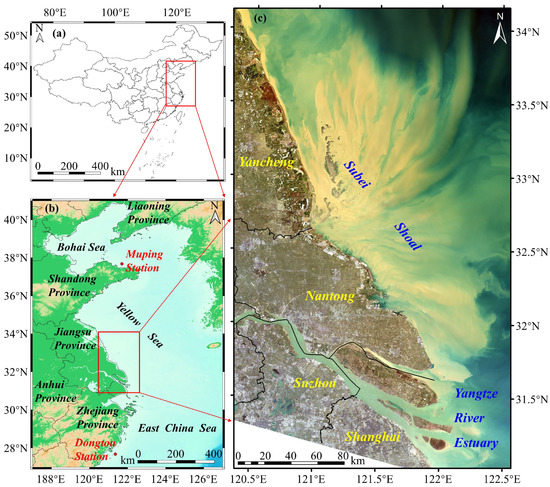
Figure 1.
Overview of the study area. (a) Location of the East China Coast in China. (b) Overview of the East China Coast. The red dots represent the calibration stations of the National Satellite Ocean Application Service in the Yellow Sea and East China Sea. Background map obtained by GEBCO (http://www.gebco.net/, last accessed on 13 July 2022). (c) Turbid water in the Subei Shoal (SBS) and the Yangtze River Estuary (YRE). The base map is the quasi-true color georeferenced HY-1C CZI image on 27 February 2022.
The YRE is a large mesotidal subtropical estuary, where a substantial volume of sediment discharge from the Yangtze River flows into the sea [8]. The developed economy and large population of the YRE region imply its fundamental socioeconomic importance, as a tidal wetland, it is also extremely important ecologically. The SPM within the YRE is highly dynamic due to complex hydrological processes.
2.2. In Situ Data
As for the apparent optical properties (AOPs), we use Hyperspectral Surface Acquisition System (HyperSAS) to in situ measure spectral radiance parameters for estimating remote-sensing reflectance (Rrs). Two radiance sensors were set away from the sun with an optimal zenith angle of 40° and an optimal azimuth angle of 135° to minimize the impact of wind speed and reduce solar glitter effects [34]. The field-measured Rrs is calculated as follows:
where Lt(λ), Ls(λ) and Ed(λ) represent the total upwelling spectral radiance, incident spectral radiance and downwelling spectral irradiance, respectively. Here, ρ(λ) is a ratio of spectral reflected sky radiance.
Water samples are collected simultaneously during field sampling, and then obtain SPM concentration after filtering, drying, weighing and other operations. The specific experimental operation was detailed in the study of Luo et al. [8].
2.3. Satellite Data
Landsat-8 and Landsat-9 satellites were launched in February 2013 and September 2021, respectively. They carried the OLI sensor with a spatial resolution of 30 m and revisit period of 16 days, the joint network operation of Landsat-9 and Landsat-8 has enabled the observation of the Earth every 8 days. OLI has a higher signal-to-noise ratios (SNR) than the thematic mapper (TM) on-board Landsat-4/5 and the enhanced thematic mapper plus (ETM+) on-board Landsat-7 [35]. Level-1 Landsat-8/9 OLI data of the SBS and YRE were downloaded from the United States Geological Survey (USGS, https://earthexplorer.usgs.gov/ (last accessed on 16 June 2022)).
HY-1C and HY-1D satellites were launched in September 2018 and June 2020, respectively, they both carried a CZI sensor with a wide swath width of about 950 km, a high spatial resolution better than 50 m, and high timeliness that can achieve twice observations in three days. Level-1 HY-1C/D CZI data of the SBS and YRE were downloaded from the National Satellite Ocean Application Service (https://osdds.nsoas.org.cn/OceanColor/ (last accessed on 12 June 2022)). The CZI sensor has four bands from visible to near-infrared, with wavelengths ranging from 0.42-0.89 μm and center wavelengths of 460, 560, 650, and 825 nm, and a quantization level of 12 bits. It is mainly used for coastal zone monitoring, understanding the distribution and change pattern of suspended matter, and to conduct real-time monitoring and early warning of marine environmental disasters such as ice disaster, red tide, green tide and pollutants.
In summary, the advantageous characteristics of HY-1C/D CZI compared with Landsat-8/9 OLI are shown in Table 1. The spectral response curves of CZI and OLI are shown in Figure S1.

Table 1.
The advantageous characteristics of the coastal zone imager (CZI) on-board HY-1C/D compared with the operational land imager (OLI) on-board Landsat-8/9.
3. Methods
In order to evaluate the potential of HY-1C/D-CZI images for quantifying SPM, it is necessary to establish accurate atmospheric correction and SPM inversion algorithms, which are described in detail below. In addition, considering that the band settings and spatial resolution of CZI and OLI are similar, this study will cross-validate the products of CZI and OLI at all levels.
3.1. Reflectance at Top of Atmosphere
The raw data received by the remote sensing sensors are stored in digital numerical (DN) format, and the downloaded DN data is converted into the zenith radiance (LTOA) through radiometric calibration:
where the DN and the corresponding gain and offset for each band are provided by the downloadable Level 1 products of CZI and OLI.
In order to eliminate the influence of solar geometric differences and solar spectral radiation differences of corresponding bands, before the comparison of OLI and CZI, the LTOA should be converted into the top-of-atmosphere reflectance (ρTOA) by Equation (3):
where E0(λ) is the average solar spectral irradiance at λ, the angle at which sunlight incident to the earth’s surface is called the solar zenith angle (θ) and d is the earth-sun distance in astronomical units (AU).
In addition, to maximize the elimination of effects such as solar zenith angle and spectral response function between OLI and CZI, the relative relationship between LTOA of CZI and OLI images was obtained using the linear relationship between ρTOA of CZI and OLI images combined with Equation (3).
where E0−OLI and E0−CZI were the average solar spectral irradiance at the equivalent wavelength of OLI and CZI sensors, θOLI and θCZI were the observed solar zenith angle of OLI and CZI sensors.
3.2. Atmospheric Correction
The total reflectance, at a wavelength λ, measured at the top of atmosphere can be expressed as [21]:
where ρrc is the Rayleigh reflectance, ρa is the aerosol reflectance, t is the diffuse transmittance, ρw is the water-leaving reflectance.
The atmospheric correction mainly includes Rayleigh scattering correction and aerosol scattering correction. Currently, the Rayleigh scattering correction can be accurately calculated through LUTs. However, in general, specific LUTs need to be generated for different sensors. The generalized Rayleigh scattering correction LUTs generated based on a vector radiative transfer model has good universality, and can meet the Rayleigh scattering correction of different sensors [36,37], which is convenient and fast to use.
The aerosol scattering correction is mainly based on NIR or SWIR dark pixel method. For the atmospheric correction of turbid water in the absence of SWIR band, ESOA provides a better solution by coupling the semi-empirical radiative transfer model applicable to highly turbid waters with the AMHAD2010 aerosol model, to solve the aerosol parameters of the image for aerosol scattering correction. Since CZI lacks the band required for the dark pixel atmospheric correction method, this study refers to the ESOA method [24], constructs a water-atmosphere coupling model suitable for CZI images, and develops the ESOA-CZI atmospheric correction method.
In short, for atmospheric correction of CZI images, this study first uses the generalized Rayleigh scattering correction LUTs to complete the Rayleigh scattering correction of CZI images, and then uses ESOA-CZI to perform aerosol scattering correction of CZI images, which will be described in detail in the following sections.
3.2.1. CZI Rayleigh Correction
Current accurate Rayleigh scattering calculations for ocean color remote sensing are usually performed using look-up tables (LUTs), but since these LUTs are generated for specific remote sensing sensors, they are difficult to be directly applied to new ocean color remote sensing sensors. For this reason, He et al. [36,37] independently-developed a vector radiative transfer model termed PCOART for the coupled ocean–atmosphere system with rough sea-surface, which solves the vector radiative transfer equation using the matrix-operator or adding-doubling method.
A comparison of the results with the SeaDAS accurate Rayleigh scattering LUTs show that the calculation accuracy of the PCOART universal LUTs were better than 0.5%, which can be used for accurate Rayleigh scattering calculations for all ocean color remote sensing sensors. Therefore, Rayleigh correction of CZI was performed using PCOART in this study. The LUTs has been operated and could be downloaded from https://www.satco2.com/index.php?m=content&c=index&a=lists&catid=399/ (last accessed on 14 July 2022).
3.2.2. CZI Aerosol Correction
Semi-Empirical Radiative Transfer Model
For turbid estuarine and coastal waters, a semi-empirical radiative transfer (SERT) model based on a two-stream approximate radiative transfer theory [38] was proposed by Shen et al. [39] for remote sensing estimation of SPM, assuming that the ratio of backscattering coefficient (bb) and absorption coefficient (a) is positively correlated with SPM, taking into account that suspended particulate matter in the water mainly has a sensitive effect on scattering, while it has little sensitive effect on absorption. The specific form of the SERT model is as follows:
where Rrs is the atmospherically corrected remote sensing reflectance in sr−1, u and v are empirical and wavelength-dependent coefficients, and SPM is the suspended particulate matter concentration in g/L.
In order to reduce the discrepancy between the CZI atmospherically corrected Rrs and the in situ measured Rrs. In this study, based on the spectral response function (SRF) of CZI, the in situ measured Rrs(λ) was converted into Rrs(λ) measured at the equivalent wavelength of CZI using Equation (8).
where Rrs(bandi) is the equivalent Rrs(sr−1) measured by the CZI for the i-th band; λ1 and λ2 are the lower and upper limits in the wavelength range for the i-th band, respectively; SRF(λ) is the spectral response function of the CZI at λ; Rrs(λ) is the in situ measured Rrs at λ.
The simultaneously simulated CZI-based derived Rrs (calculated by Equation (8)) and SPM datasets (716 samples) from multiple cruises in the estuarine and coastal waters were available for the determination of fitting parameters u and v of the SERT model based on the least-squares method according to Equation (7). In this study, the SERT model after fitting the sensor equivalent wavelength and re-optimizing the calibration parameters is referred to as the SERT_c model. The wavelength-dependent u and v are listed in Table 2, the results show that the SERT_c model has higher accuracy in the red and near-infrared bands.
Table 2.
u and v coefficients of the SERT_c model for CZI data.
Implementation of ESOA_CZI Based on a Genetic Algorithm
The sum of the aerosol reflectance ρa(λ) and the normalized water-leaving reflectance [ρw(λ)]N at the zenith is expressed as ρaw(λ):
where ts(λ) and tv(λ) represent the diffuse transmittance in the solar direction and the sensor observation direction, respectively.
Based on the definition of normalized water-leaving reflectance [ρw(λ)]N and remote sensing reflectance Rrs(λ), it is easy to derive Equation (10):
The AHMAD2010 aerosol model [40] and the SERT water radiative transfer model were used to calculate ρa(λ), ts(λ), tv(λ) and Rrs(λ), respectively, and then ρaw(λ) can be calculated by coupling Equations (9) and (10).
In addition, the top-of-atmosphere reflectance ρTOA can be linearly expressed as the sum of the reflectivity of each part. In this study, the ρTOA(λ) after Rayleigh scattering (ρrc(λ)), white cap reflection ρwc(λ), and flare reflection ρglint(λ) correction is expressed by ρn(λ):
where T(λ) represent the solar direct transmittance. Note that in the Equation (11), we ignore the sea surface reflectance from whitecaps and sun-glint [41].
In theory, ρn(λ) is equal to ρaw(λ) at all wavelengths, so combined with the above sea- atmosphere coupling model, we developed a system of nonlinear equations for CZI sensors:
where RH and FMF represent relative humidity and fine-mode fraction, respectively.
The unknown variables which are relative humidity (RH) and fine-mode fraction (FMF) that determine the aerosol type, the aerosol optical thickness at the reference wavelength τa(λ0) and SPM, are estimated from nonlinear equations (Equation (12)).
Due to the large spatial and temporal variability of SPM and aerosol optical properties in the SBS and YRE, it is difficult for SOA2009 [42] and its previous spectral optimization algorithms to accurately estimate the initial values of the four unknown variables in Equation (12). Genetic Algorithm (GA) is a global optimization algorithm that has been widely adopted and does not depend on the initial estimation of the unknown variables. For the solution of a specific problem, GA requires the determination of three main aspects: the ranges and encodings of the variables, the determination of the objective function, and the selection of the genetic operator algorithm and important parameters. The main parameters of GA model for CZI are the same as those set by Pan et al. [24] for GOCI. Therefore, in this study, GA is used to optimally solve for the variables of Equation (12).
3.2.3. OLI Atmospheric Correction
The ACOLITE bundles the atmospheric correction algorithms and processing software for aquatic applications of high-resolution satellite data, especially suited for processing of turbid waters, The ACOLITE performs well for atmospheric correction over turbid estuarine and coastal waters [8,43]. The Level-1 Landsat-8/9 OLI data were processed using the open-source ACOLITE software (version 20220222.0), in combination with the dark spectrum fitting (DSF) algorithm (with glint correction), to obtain ρTOA and remote sensing reflectance (Rrs) [44].
3.3. Inversion of Suspended Particulate Matter Concentration
The study area of this paper is the Subei Shoal and the Yangtze River Estuary, which are located in the estuarine and coastal areas, where SPM in the waters is dominant, leading to high turbidity of the waters, and drastic changes in SPM dynamics. Therefore, it is of great significance to monitor SPM in this region using remote sensing data with high spatial resolution. Meanwhile, for turbid waters, Rrs is mainly affected by SPM, and the inversion algorithm of SPM is relatively mature. In addition, CZI only sets four bands of 460 nm, 560 nm, 650 nm and 825 nm, which makes it difficult and low accuracy to invert other ocean color parameters (such as chlorophyll a, CDOM, etc.).
The suspended particulate matter concentration in the SBS and YRE was retrieved by implementing the SERT_c model (Section 3.2.2) to the atmospherically corrected Rrs images of CZI and OLI. The 716 sets of Rrs and SPM matched datasets were collected simultaneously in the estuarine and coastal areas in recent years and divided into modeling and validation datasets according to 8:2 for the SERT_c model (Figure 2). The results show a high coefficient of determination of 0.91 for the Rrs and SPM modeling datasets (N = 572), while the mean absolute error of the validation dataset (N = 144) is below 0.0731 g/L.
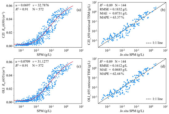
Figure 2.
Development (left) and validation (right) of the SERT_c model. (a,b) HY-1C/D CZI sensor, (c,d) Landsat-8/9 OLI sensor.
In addition, the original SERT model was validated using the same validation dataset (Figure S2), and the comparison results showed that the accuracy of the SERT_c model to retrieve the SPM concentration was better than that of the SERT model. In the practical application of remote sensing images, the inverse form of SERT_c model is shown as follows:
where for the red band of the CZI sensor, u is 0.0697 and v is 32.7876 (Figure 2a); for the red band of the OLI sensor, u is 0.0709 and v is 31.1277 (Figure 2c).
3.4. Accuracy Evaluation
The values of CZI images and OLI images can be compared based on the numerous methods or indicators available to assess the agreement between two data sets. The International Ocean Color Coordination Group (IOCCG) recommends the mean absolute percentage error (MAPE), the root mean square error (RMSE), the coefficient of determination R2, defined as (Pearson coefficient), or the slope and intercept of linear regression [45]. MAPE and RMSE were obtained according to Equations (14) and (15), respectively.
where X represents a variable (e.g., ρTOA, Rrs, SPM), n is the number of samples, and the superscripts estimated and measured represent the estimated and measured values, respectively.
4. Results
To evaluate the effect of ESOA_CZI atmospheric correction and the potential of CZI to estimate SPM, this study uses OLI data to cross-validate with CZI data products at all levels, and assists in verification with in situ data. Considering the difference in transit time (about 30 min), as well as the difference in spectral response functions of each band, combined with the difference of some other factors between CZI and OLI, these are not conducive to the direct comparison between them. Therefore, before the cross-comparison between CZI and OLI, CZI was relatively corrected using the linear relationship between the original LTOA of CZI and OLI, and the angular information such as solar zenith angle is also consistent with OLI, so that the input atmospheric correction parameters are consistent as much as possible to better test the effect of ESOA_CZI atmospheric correction. Meanwhile, CZI uses the nearest-neighbor image element method to resample to a spatial resolution of 30 m × 30 m in order to generate a uniform resolution dimension with OLI images. In addition, the blue band is not considered in this study because of its atmospheric correction instability.
4.1. Comparison of TOA Reflectance between CZI and OLI
In this study, cloud-free CZI and OLI images covering the SBS and YRE were collected on 27 February 2022. Figure 3 shows that the ρTOA of CZI and OLI have strong correlation, specifically, from low to high reflectance in all three bands (green, red, NIR) showing a good linear relationship. Therefore, the CZI image can satisfy the need for satellite Rrs observations in waters with different turbidity by using suitable atmospheric correction process. Among them, the best results were obtained for ρTOA in the red band, the slope of their linear regression fitting line was closer to 1, the intercept was smaller, and the distribution of its results was closer to the 1:1 line. In addition, the coefficient of determination was as high as 0.9803 (n = 38331813), with the smaller RMSE and MAPE of 0.0050 W m−2 μm−1 and 5.01%, respectively. The overall results of ρTOA in the green and near-infrared bands are good, although the ρTOA of CZI is a little high in the green band and a little low in the high reflectance part of ρTOA in the NIR band.
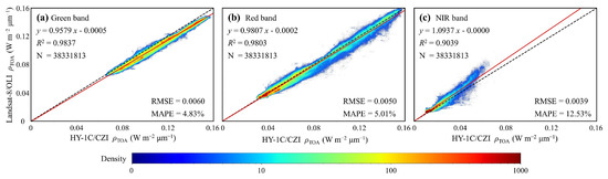
Figure 3.
Scatterplots of CZI versus OLI of TOA reflectance at the green (a), red (b) and NIR (c) bands on 27 February 2022 in the SBS and YRE, respectively.
4.2. Rrs Comparison and Validation
The Rrs of the waters were obtained after atmospheric correction of ρTOA. Figure 4 shows the good linear relationship of Rrs in green, red and NIR bands of CZI and OLI images. The results show that the Rrs between CZI and OLI in the red band have good agreement (R2 = 0.9761), low RMSE (0.0020 sr−1) and low MAPE (18.10%), the Rrs values derived from the red band in CZI and OLI data were basically equal (Figure 4b). Large MAPE values are observed in the NIR band (Figure 4c), where the reason could be that the Rrs is close to zero in the low value part of Rrs, while the Rrs of OLI is large in the high value part of Rrs. For the green band, the low Rrs value part of CZI is lower than that of OLI (Figure 4a).
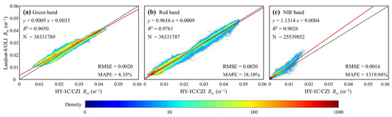
Figure 4.
Scatterplots of CZI versus OLI of Rrs at the green (a), red (b) and NIR (c) bands on 27 February 2022 in the SBS and YRE, respectively.
In order to further test the atmospheric correction performance of the ESOA_CZI algorithm, we collected in situ measured quasi-synchronous Rrs data from two calibration stations (Muping station (121°42′00″E, 37°40′51.6″N) and Dongtou station (121°21′18″E, 27°40′30″N)) of the National Satellite Ocean Application Service for verification. First, all the in situ Rrs data of the two stations obtained from September 2019 to June 2022 were matched with the CZI images, and we select the Rrs data whose time window between the sampling time of in situ measurement and the transit time of the HY-1C/D is less than half an hour. Next, the CZI-derived Rrs values were obtained by taking the location of the calibration station as the central pixel and combining 8 surrounding pixels to form a 3 × 3 grid, and calculating the average value of Rrs within the grid. Quality control was performed before processing according to the rule that the effective pixels in the grid were more than 8 and the coefficient of variation was less than 15%.
Since the wavelengths of the in situ Rrs at the calibration stations do not exactly coincide with the central wavelengths of CZI at 460, 560, 650 and 825 nm, which the closest corresponding wavelengths are 490, 560, 667 and 779 nm. Therefore, we used 716 hyperspectral Rrs data measured on multiple cruises in estuarine and coastal areas, and also to reduce the error between the measured hyperspectral Rrs data and CZI multispectral Rrs data, the hyperspectral Rrs data were fitted to the corresponding center wavelength of CZI band based on the spectral response function of CZI. Next, the linear relationships between the CZI-based fitted Rrs at 460, 560, 650 and 825 nm and the corresponding in situ measured at 490, 560, 667 and 779 nm were established, respectively, and the in situ Rrs from two calibration stations at 490, 560, 667 and 779 nm were corrected and migrated to Rrs at 460, 560, 650 and 825 nm using these linear relationships. Finally, 28 matchups of satellite data and simultaneous in situ data were successfully obtained, and the mean values of the in situ Rrs from two calibration stations at 460, 560, 650 and 825 nm were 0.0135 sr−1, 0.0201 sr−1, 0.0107 sr−1 and 0.0015 sr−1, respectively, with the corresponding coefficients of variation were 30.72%, 39.85%, 76.54% and 143.53%, respectively.
Finally, the scatter plots of the in situ measured Rrs and CZI-derived Rrs at 560, 650 and 825 nm was shown in Figure 5. As mentioned before, due to the poor atmospheric correction effect of the blue band (460 nm), it is not involved in the comparison here. The results are as follows: the R2 values of the CZI-derived Rrs and the in situ measured Rrs at green (560 nm), red (650 nm) and NIR (825 nm) bands were 0.8040, 0.8810 and 0.5295, respectively. In addition, the RMSE were 0.0036 sr−1, 0.0035 sr−1 and 0.0045 sr−1, respectively. Furthermore, the MAPE were 0.1844%, 0.6239% and 91.1752%, respectively. Most of the data are concentrated around the 1:1 line and no negative values were obtained, which indicates that ESOA_CZI algorithm performs well in these bands.
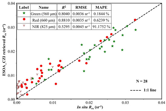
Figure 5.
Comparison of CZI-retrieved Rrs by ESOA_CZI algorithms with in situ Rrs data.
These results show that ESOA_CZI algorithm has the ability to accurately realize the atmospheric correction of CZI, even in estuarine and coastal waters with large spatio-temporal dynamic changes, coexistence of clear water and turbid water, and complex optical properties. More importantly, the red band (650 nm) used to estimate SPM in this study has the highest R2 (0.8810) and the smallest RMSE (0.0035 sr−1), and its results are also basically distributed along the 1:1 line. Combining the SERT_c algorithm with strong robustness to estimate the SPM of estuarine and coastal waters has great development potential and broad application prospects.
4.3. Comparison and Validation of CZI and OLI for Quantifying SPM
According to the results of Rrs after CZI atmospheric correction, it can be seen that Rrs in the red band has the best effect. Moreover, the Rrs in the green band is not sensitive to the change of SPM and is easy to saturate. However, the Rrs in the NIR band is less stable and likely to have negative values in the clear water area. Therefore, to illustrate the accuracy of CZI and OLI images inversion of SPM, only red band was selected to input into SERT_c model to invert SPM. The cross-comparison scatter plot of CZI and OLI image inversions of SPM are shown in Figure 6. The results show that the SPM concentration of CZI inversion was highly consistent with that of OLI inversion (R2 = 0.9481), and the slope of their linear regression fitting line was very close to 1 (slope = 0.9870), the intercept was as low as 0.0006 g/L, the RMSE was only 0.0167 g/L, and the MAPE was 26.39%. This shows that it is feasible and reliable to estimate SPM of SBS and YRE by SERT_c model using ESOA_CZI atmospheric corrected Rrs, and the future application of CZI images to long time series and large-scale SPM observation of estuarine and coastal waters has great value and potential.
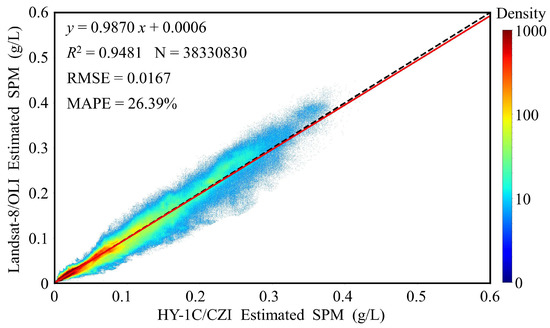
Figure 6.
Scatterplots of CZI and OLI of SPM on 27 February 2022 in the SBS and YRE.
The SPM results of SBS and YRE estimated from CZI and OLI images on 27 February 2022 are shown in Figure 7. The spatial distribution of SPM estimated from CZI and OLI images has good consistency, and both reflect the distribution pattern of SPM in the SBS and YRE waters. Compared with the medium-resolution images, the high-resolution images can observe the dynamic changes of SPM around the nearshore, islands and tidal flats, as well as details such as fine eddies in the water and the wake of ships.
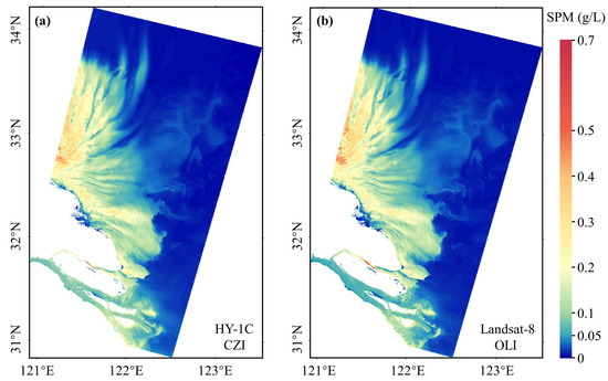
Figure 7.
SPM distribution in the SBS and YRE estimated by using SERT_c model based on CZI images (a) and OLI images (b) on 27 February 2022.
To further test the performance of the CZI image quantifying SPM, we selected the SPM data quasi-synchronous (within one hour) with the local transit time of CZI images from the in situ measured SPM datasets for verification, and a total of 16 sets of SPM data were matched (Figure 8). The verification results show that the R2 values was 0.86, the RMSE was 0.0362 g/L, and the MAPE was 33.21%. Most of the data are concentrated around the 1:1 line, which indicates that the CZI images are capable of estimating the SPM distribution and variability in estuarine and coastal waters by ESOA_CZI atmospheric correction and SERT_c inversion SPM algorithm.
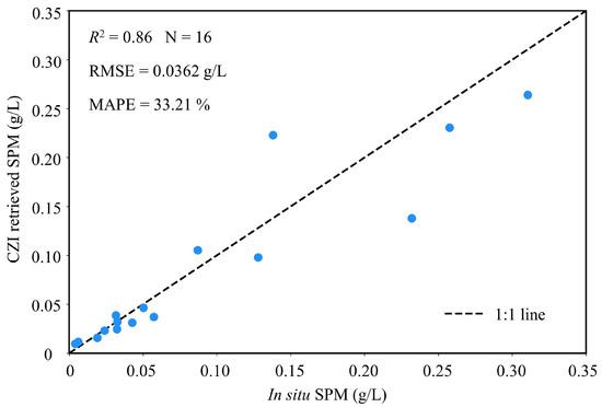
Figure 8.
Scatter plots of comparisons between CZI-retrieved SPM and in situ SPM.
4.4. CZI Images for Quantifying SPM
Taking advantage of the short revisit period of CZI images that can achieve 6 observations in 7 days for the SBS and YRE regions (Figure 9). Combine with the advantages of 50 m resolution and wide width, CZI images has great advantage and potential in estimating the SPM of estuarine and coastal areas. As shown in Figure 9, the spatial and temporal dynamics of SPM in SBS and YRE vary greatly, and the SPM generally shows a distribution pattern of decreasing from west (coastal) to east (open sea) and decreasing from north (SBS) to south (YRE). The SPM concentration in the coastal area of Yancheng and the waters adjacent to the radial sand ridge group of SBS is the highest, generally greater than 0.7 g/L. The SPM concentration in the coastal area of Nantong to the south decreases to about 0.3–0.7 g/L, and the SPM concentration in the maximum turbidity zone of the YRE in the further south is only about 0.2–0.4 g/L, and the SPM concentration in the upper section of YRE is as low as 0.05–0.2 g/L. The SPM concentration in the outer sea is even lower, roughly below 0.05 g/L.
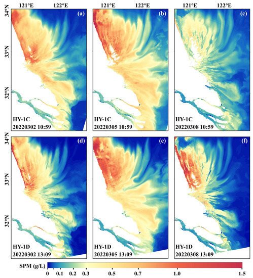
Figure 9.
Temporal and spatial dynamics of SPM in SBS and YRE were observed using CZI images. HY-1C (a) and HY-1D (d) CZI image on 2 March 2022; HY-1C (b) and HY-1D (e) CZI image on 5 March 2022; HY-1C (c) and HY-1D (f) CZI image on 8 March 2022.
Interestingly, the SPM plume with distinctive features often appears in the sea area east of the radial sand ridge group in the SBS, which are particularly spectacular and beautiful natural scenery, which may be formed by the action of underwater topography and tidal current. The water level caused by flood and ebb tides directly determines the size of the exposed tidal flats in the radial sand ridge group. Generally, the tidal flats have a large, exposed area and low SPM concentration at low tide level (Figure 9c), while the tidal flats are flooded and have high SPM concentration at high tide level (Figure 9e), which may be caused by the resuspension of the substrate in the shallows due to strong tidal power.
4.5. Advantages of Fine Spatial Resolution
Spatial resolution has a significant effect on the imaging accuracy of objects with high spatial variability, and to quantify the differences in feature observations by sensors with different spatial resolutions, the coefficient of variation (CV) is used to measure the amount of information contained within the waters observed by the sensor:
where SD is the standard deviation, and MN is the mean value.
An HY-1C/CZI image of SBS local area in 27 February 2022 was selected. Details such as groin, vegetation, clear water areas and turbid water zones with different turbidity levels can be clearly seen from the RGB true color image with a spatial resolution of 50 m (Figure 10a). Figure 10b–d showed the original image of red band (650 nm) with a spatial resolution of 50 m, and resized image with spatial resolution of 100 m and 500 m. The cross-comparison of the LTOA in this region of different spatial resolution is shown in Figure 10e,f.
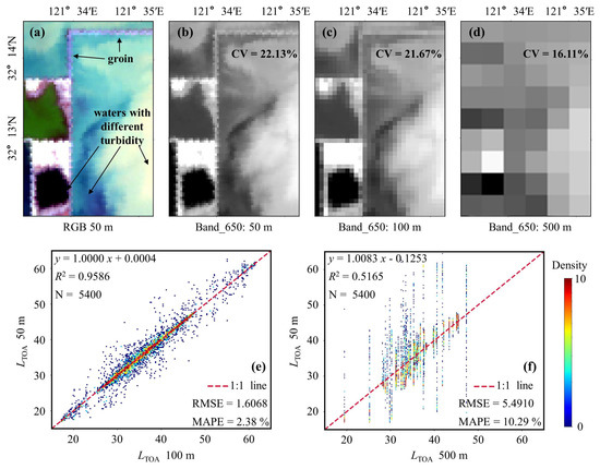
Figure 10.
Comparison of original and resized HY-1C/CZI image of SBS local area in 27 February 2022: (a) RGB true color image with spatial resolution of 50 m, (b) original red band image (50m), (c) resized red band image (100 m), (d) resized red band image (500 m). (e) density scatter plots between 50 m resolution and 100 m resolution, (f) density scatter plots between 50 m resolution and 500 m resolution.
50 m spatial resolution image are sufficient to distinguish small-scale objects such as groin, sea reclamation boundary, etc. (Figure 10b), while 500 m resolution image cannot observe the details of these features (Figure 10d). Some studies have shown that the optimal scale observation of estuarine and coastal areas should be less than 100 m, or even less than 50 m in some cases [46]. The results of cross-comparison of images with different spatial resolutions show that the reduction in spatial resolution results in significant errors (Figure 10e,f). In addition, when the resolution decreases, the information and details of remote sensing data are gradually lost, and the CV values in the region gradually decreases from 22.13% for 50 m resolution images to 16.11% for 500 m resolution images (Figure 10b–d). Therefore, compared with the spatial resolution of water color sensors at the level of hundred meters, the spatial resolution of CZI at 50 m has an incomparable advantage in observing information and details of estuarine and coastal areas.
5. Discussion
Compared with other remote sensing sensors, HY-1C/D CZI combines the advantages of high spatial resolution (50 m), high temporal resolution (2 observations in 3 days) and wide swath width (950 km), which has unparalleled advantages for monitoring estuarine and coastal waters with large dynamic changes and complex optical properties [12]. Specifically, only 9 CZI images are needed to cover the whole estuarine and coastal waters of China, while at least 46 OLI images or more MSI images are needed. The combined HY-1C/D network is capable of 10 or 12 observations in 16 days, with observations in both morning and afternoon, while the combined Landsat-8/9 network is capable of only 2 observations in 16 days, with no observation in the afternoon.
The premise of CZI application in ocean color observation is the development of a reliable atmospheric correction algorithm [12,13], so the ESOA_CZI algorithm was proposed in this study. The reason why selecting OLI data for cross-validation is that OLI and CZI have similar band settings and similar spatial resolution (Table 1), and previous studies have shown that OLI can be applied to retrieve ocean color parameters with good results [8]. However, it is difficult to achieve complete synchronization between CZI and OLI, i.e., the difference in observation time between the 2 sensors is roughly half an hour, which will inevitably cause angular differences such as the solar zenith angle, and the estuarine and coastal waters also have certain variations within half an hour under the influence of ocean currents. At the same time, the spectral response functions of the two sensors are also different Figure S1. Therefore, if a systematic correction of the LTOA of CZI is required, it is necessary to make a linear correction by the ρTOA of CZI and OLI (Equation (4)) and decompose the effect of the solar zenith angle and the spectral response function (Equation (5)). In theory, the linear relationship between the ρTOA of CZI and OLI can be used to recalibrate the LTOA to give specific and fixed calibration coefficients. Unfortunately, in practice, the LTOA correction coefficients between CZI and OLI sensors are found to be somewhat different after comparing multiple sets of images at different times, which may be that the sensors have some performance degradation in different periods or the atmospheric environment parameters such as aerosols are different when imaging in different seasons. Therefore, this study uses the linear relationship between the original LTOA of CZI and OLI to make a relative LTOA correction of CZI, and ensures that the angle information such as solar zenith angle was also consistent with OLI, so that the input atmospheric correction parameters are consistent. The results show that the Rrs obtained by CZI using ESOA_CZI maintain good agreement with those obtained by OLI using Acolite software (Figure 4), which proves that ESOA_CZI atmospheric correction algorithm is feasible and has high accuracy, especially in the green and red bands. The main reason for the large difference of Rrs in the NIR band may be that the wavelength difference of the CZI and OLI in the NIR band is 40 nm, which leads to a certain degree of unsatisfactory effect of LTOA linear correction.
Usually in the blue band, more than 80% of the total signal received by the satellite is due to the confounding influences of the atmosphere [21], this may be the reason for the poor atmospheric correction effect of the ESOA_CZI algorithm at blue wavelengths. The large dynamic variation of SPM in estuarine and coastal waters is the combined result of the stochastic processes of sediment movement, the heterogeneity of underwater topography, the seasonal variations of runoff and wind, and the periodic movements of tidal currents and waves, making it challenging to observe SPM in estuarine and coastal waters [8,43,47]. Therefore, we have developed atmospheric correction methods and SPM estimation models suitable for CZI images. The atmospheric correction results at green, red and NIR bands (Figure 4 and Figure 5) and the effect of SPM inversion (Figure 6, Figure 7 and Figure 8) show that the CZI has the potential to provide high-quality ocean color products for scientific research and society-level applications.
6. Conclusions
In order to take advantage of the high spatial resolution, high temporal resolution and large scene size of HY-1C/D CZI, and to exploit the potential of CZI quantitative inversion of ocean color products, this paper proposes a new atmospheric correction algorithm ESOA_CZI for CZI images applicable to turbid water in estuarine and coastal zone. The algorithm was firstly based on the vector radiative transfer model termed PCOART to calculate CZI Rayleigh scattering reflectance. Next, a semi-empirical radiative transfer model with suspended particle concentration as the parameter is used to model the water-atmosphere coupling. Finally, the parameters of the coupling model are solved by combining a global optimization approach that is based on a genetic algorithm.
The accuracy of the ESOA_CZI algorithm was verified using the quasi-synchronous OLI data and the in situ data from the calibration station. Comparison with the OLI-derived Rrs showed that the CZI-derived Rrs have good consistency in the green and red bands, especially in the red band, which maintains high consistency (R2 = 0.9761), low RMSE (0.0020 sr−1) and low MAPE (18.10%). Compared with the in situ data, the RMSE were 0.0036 sr−1 and 0.0035 sr−1, and the MAPE were 0.1844% and 0.6239%, respectively, for CZI-derived Rrs in the green and red bands.
The values and spatial distributions of CZI-estimated SPM and OLI-estimated SPM in YRE and SBS are basically consistent, and the validation using in situ data revealed that the inversion of SPM concentration by CZI was effective (R2=0.86, RMSE=0.0362 g/L). CZI has higher revisit period and wider swath width than OLI, which can better reflect the rapid spatial change characteristics of ocean color in the estuarine and coastal waters. In the future, CZI will have broad application prospects in monitoring ocean color constituents in estuarine and coastal waters in China and even the world, such as obtaining the SPM distribution of estuarine and coastal waters, and estimating the suspended sediment flux and carbon flux, which will provide data support and scientific basis for formulating and implementing the development, utilization and protection strategy of estuarine and coastal zone.
Supplementary Materials
The following supporting information can be downloaded at: https://www.mdpi.com/article/10.3390/rs15020386/s1, Figure S1: Spectral response curves of CZI band (solid line) and OLI band (dashed line); Figure S2: Validation of the SERT model. (a) HY-1C/D CZI sensor, (b) Landsat-8/9 OLI sensor.
Author Contributions
F.S. conceived and organized the research activity. W.L. conducted the data collection, processing, analysis and manuscript writing. R.L. and W.L. wrote the programs to perform atmospheric correction and data processing for CZI, J.L. worked on the data collecting and advised the research project. All authors checked the language and the figures of the article and agreed to the published version of the manuscript.
Funding
This research was supported by the National Natural Science Foundation of China (Nos. 42271348 and 42076187).
Data Availability Statement
Not applicable.
Acknowledgments
The National Satellite Ocean Application Service, MNR of PRC, are thanked for the HY-1C/D CZI imagery and Rrs data from two calibration stations. The USGS and NASA are acknowledged for their Landsat-8/9 OLI imagery. The Remote Sensing and Ecosystem Modelling (REMSEM) team of the Royal Belgian Institute of Natural Sciences is thanked for the ACOLITE software.
Conflicts of Interest
The authors declare no conflict of interest.
References
- Liu, J.A.; Liu, D.; Du, J. Radium-traced nutrient outwelling from the Subei Shoal to the Yellow Sea: Fluxes and environmental implication. Acta Oceanol. Sin. 2022, 41, 12–21. [Google Scholar] [CrossRef]
- Zhao, S.; Xu, B.; Yao, Q.; Burnett, W.C.; Charette, M.A.; Su, R.; Lian, E.; Yu, Z. Nutrient-rich submarine groundwater discharge fuels the largest green tide in the world. Sci. Total Environ. 2021, 770, 144845. [Google Scholar] [CrossRef] [PubMed]
- Guo, L.; Zhu, C.; Xie, W.; Xu, F.; Wu, H.; Wan, Y.; Wang, Z.; Zhang, W.; Shen, J.; Wang, Z.B.; et al. Changjiang Delta in the Anthropocene: Multi-scale hydro-morphodynamics and management challenges. Earth Sci. Rev. 2021, 223, 103850. [Google Scholar] [CrossRef]
- Arena, M.; Pratolongo, P.; Delgado, A.L.; Celleri, C.; Vitale, A. Spatial and temporal distribution of satellite turbidity in response to different environmental variables in the Bahía Blanca Estuary, South-Western Atlantic. Int. J. Remote Sens. 2022, 43, 3714–3743. [Google Scholar] [CrossRef]
- Chen, S.; Zhang, G.; Yang, S.; Shi, J.Z. Temporal variations of fine suspended sediment concentration in the Changjiang River estuary and adjacent coastal waters, China. J. Hydrol. 2006, 331, 137–145. [Google Scholar] [CrossRef]
- Cai, L.; Chen, S.; Yan, X.; Bai, Y.; Bu, J. Study on High-Resolution Suspended Sediment Distribution under the Influence of Coastal Zone Engineering in the Yangtze River Mouth, China. Remote Sens. 2022, 14, 486. [Google Scholar] [CrossRef]
- Tang, R.; Shen, F.; Ge, J.; Yang, S.; Gao, W. Investigating typhoon impact on SSC through hourly satellite and real-time field observations: A case study of the Yangtze Estuary. Cont. Shelf Res. 2021, 224, 104475. [Google Scholar] [CrossRef]
- Luo, W.; Shen, F.; He, Q.; Cao, F.; Zhao, H.; Li, M. Changes in suspended sediments in the Yangtze River Estuary from 1984 to 2020: Responses to basin and estuarine engineering constructions. Sci. Total Environ. 2022, 805, 150381. [Google Scholar] [CrossRef] [PubMed]
- Pahlevan, N.; Smith, B.; Alikas, K.; Anstee, J.; Barbosa, C.; Binding, C.; Bresciani, M.; Cremella, B.; Giardino, C.; Gurlin, D.; et al. Simultaneous retrieval of selected optical water quality indicators from Landsat-8, Sentinel-2, and Sentinel-3. Remote Sens. Environ. 2022, 270, 112860. [Google Scholar] [CrossRef]
- Vanhellemont, Q.; Ruddick, K. Turbid wakes associated with offshore wind turbines observed with Landsat 8. Remote Sens. Environ. 2014, 145, 105–115. [Google Scholar] [CrossRef]
- Estrella, E.H.; Gilerson, A.; Foster, R.; Groetsch, P. Spectral decomposition of remote sensing reflectance variance due to the spatial variability from ocean color and high-resolution satellite sensors. J. Appl. Remote Sens. 2021, 15, 24522. [Google Scholar] [CrossRef]
- Tong, C.; Mu, B.; Liu, R.; Ding, J.; Zhang, M.; Xiao, Y.; Liang, X.; Chen, X. Atmospheric Correction Algorithm for HY-1C CZI over Turbid Waters. J. Coast. Res. 2019, 90, 156–163. [Google Scholar] [CrossRef]
- Men, J.; Liu, J.; Xia, G.; Yue, T.; Tong, R.; Tian, L.; Arai, K.; Wang, L. Atmospheric correction for HY-1C CZI images using neural network in western Pacific region. Geo-spatial Inf. Sci. 2022, 25, 476–488. [Google Scholar] [CrossRef]
- Huang, Y.Y.; Tang, S.L.; Wu, J. A chlorophyll-a retrieval algorithm for the Coastal Zone Imager (CZI) onboard the HY-1C satellite in the Pearl River Estuary, China. Int. J. Remote Sens. 2021, 42, 8365–8379. [Google Scholar] [CrossRef]
- Cheng, Y.; Sun, Y.; Peng, L.; He, Y.; Zha, M. An Improved Retrieval Method for Porphyra Cultivation Area Based on Suspended Sediment Concentration. Remote Sens. 2022, 14, 4338. [Google Scholar] [CrossRef]
- Zhu, X.; Lu, Y.; Liu, J.; Ju, W.; Ding, J.; Li, M.; Suo, Z.; Jiao, J.; Wang, L. Optical Extraction of Oil Spills from Satellite Images Under Different Sunglint Reflections. Ieee T. Geosci. Remote. 2022, 60, 1–14. [Google Scholar] [CrossRef]
- Zhao, X.; Liu, R.; Ma, Y.; Xiao, Y.; Ding, J.; Liu, J.; Wang, Q. Red Tide Detection Method for HY−1D Coastal Zone Imager Based on U−Net Convolutional Neural Network. Remote Sens. 2022, 14, 88. [Google Scholar] [CrossRef]
- Ji, H.; Tian, L.; Li, J.; Tong, R.; Guo, Y.; Zeng, Q. Spatial–Spectral Fusion of HY-1C COCTS/CZI Data for Coastal Water Remote Sensing Using Deep Belief Network. IEEE J. Stars. 2021, 14, 1693–1704. [Google Scholar] [CrossRef]
- Pahlevan, N.; Mangin, A.; Balasubramanian, S.V.; Smith, B.; Alikas, K.; Arai, K.; Barbosa, C.; Bélanger, S.; Binding, C.; Bresciani, M.; et al. ACIX-Aqua: A global assessment of atmospheric correction methods for Landsat-8 and Sentinel-2 over lakes, rivers, and coastal waters. Remote Sens. Environ. 2021, 258, 112366. [Google Scholar] [CrossRef]
- Gordon, H.R. Atmospheric correction of ocean color imagery in the Earth Observing System era. J. Geophys. Res. Atmos. 1997, 102, 17081–17106. [Google Scholar] [CrossRef]
- Gordon, H.R.; Wang, M. Retrieval of water-leaving radiance and aerosol optical thickness over the oceans with SeaWiFS: A preliminary algorithm. Appl. Opt. 1994, 33, 443–452. [Google Scholar] [CrossRef]
- Vanhellemont, Q.; Ruddick, K. Atmospheric correction of Sentinel-3/OLCI data for mapping of suspended particulate matter and chlorophyll-a concentration in Belgian turbid coastal waters. Remote Sens. Environ. 2021, 256, 112284. [Google Scholar] [CrossRef]
- Xu, Y.; He, X.; Bai, Y.; Wang, D.; Zhu, Q.; Ding, X. Evaluation of Remote-Sensing Reflectance Products from Multiple Ocean Color Missions in Highly Turbid Water (Hangzhou Bay). Remote Sens. 2021, 13, 4267. [Google Scholar] [CrossRef]
- Pan, Y.; Shen, F.; Verhoef, W. An improved spectral optimization algorithm for atmospheric correction over turbid coastal waters: A case study from the Changjiang (Yangtze) estuary and the adjacent coast. Remote Sens. Environ. 2017, 191, 197–214. [Google Scholar] [CrossRef]
- Vanhellemont, Q.; Ruddick, K. Advantages of high quality SWIR bands for ocean colour processing: Examples from Landsat-8. Remote Sens. Environ. 2015, 161, 89–106. [Google Scholar] [CrossRef]
- Wang, M. Estimation of ocean contribution at the MODIS near-infrared wavelengths along the east coast of the U.S.: Two case studies. Geophys. Res. Lett. 2005, 32. [Google Scholar] [CrossRef]
- Werdell, P.J.; Franz, B.A.; Bailey, S.W. Evaluation of shortwave infrared atmospheric correction for ocean color remote sensing of Chesapeake Bay. Remote Sens. Environ. 2010, 114, 2238–2247. [Google Scholar] [CrossRef]
- Wang, M.; Shi, W. The NIR-SWIR combined atmospheric correction approach for MODIS ocean color data processing. Opt. Express. 2007, 15, 15722–15733. [Google Scholar] [CrossRef]
- Wang, J.; Lee, Z.; Wang, D.; Shang, S.; Wei, J.; Gilerson, A. Atmospheric correction over coastal waters with aerosol properties constrained by multi-pixel observations. Remote Sens. Environ. 2021, 265, 112633. [Google Scholar] [CrossRef]
- Wang, J.; Wang, Y.; Lee, Z.; Wang, D.; Chen, S.; Lai, W. A revision of NASA SeaDAS atmospheric correction algorithm over turbid waters with artificial Neural Networks estimated remote-sensing reflectance in the near-infrared. Isprs J. Photogramm. 2022, 194, 235–249. [Google Scholar] [CrossRef]
- Miao, X.; Xiao, J.; Xu, Q.; Fan, S.; Wang, Z.; Wang, X.; Zhang, X. Distribution and species diversity of the floating green macroalgae and micro-propagules in the Subei Shoal, southwestern Yellow Sea. Peer J. 2020, 8, e10538. [Google Scholar] [CrossRef]
- Xiao, J.; Fan, S.; Wang, Z.; Fu, M.; Song, H.; Wang, X.; Yuan, C.; Pang, M.; Miao, X.; Zhang, X. Decadal characteristics of the floating Ulva and Sargassum in the Subei Shoal, Yellow Sea. Acta Oceanol. Sin. 2020, 39, 1–10. [Google Scholar] [CrossRef]
- Yuan, D.; Li, Y.; Wang, B.; He, L.; Hirose, N. Coastal circulation in the southwestern Yellow Sea in the summers of 2008 and 2009. Cont. Shelf Res. 2017, 143, 101–117. [Google Scholar] [CrossRef]
- Mobley, C.D. Estimation of the remote-sensing reflectance from above-surface measurements. Appl. Opt. 1999, 38, 7442. [Google Scholar] [CrossRef] [PubMed]
- Sun, D.; Chen, Y.; Wang, S.; Zhang, H.; Qiu, Z.; Mao, Z.; He, Y. Using Landsat 8 OLI data to differentiate Sargassum and Ulva prolifera blooms in the South Yellow Sea. Int. J. Appl. Earth Obs. 2021, 98, 102302. [Google Scholar] [CrossRef]
- He, X.; Bai, Y.; Zhu, Q.; Gong, F. A vector radiative transfer model of coupled ocean–atmosphere system using matrix-operator method for rough sea-surface. J. Quant. Spectrosc. Radiat. Transf. 2010, 111, 1426–1448. [Google Scholar] [CrossRef]
- He, X.Q.; Pan, D.L.; Bai, Y.; Gong, F. General purpose exact Rayleigh scattering look-up table for ocean color remote sensing. Acta Oceanol. Sin. 2006, 25, 48–56. [Google Scholar]
- Kubelka, P.; Munk, F. Ein Beitrag Zur Optik der Farbanstriche. Z. Tech. Physik. 1931, 12, 593–601. [Google Scholar]
- Shen, F.; Verhoef, W.; Zhou, Y.; Salama, M.S.; Liu, X. Satellite Estimates of Wide-Range Suspended Sediment Concentrations in Changjiang (Yangtze) Estuary Using MERIS Data. Estuar. Coast. 2010, 33, 1420–1429. [Google Scholar] [CrossRef]
- Ahmad, Z.; Franz, B.A.; McClain, C.R.; Kwiatkowska, E.J.; Werdell, J.; Shettle, E.P.; Holben, B.N. New aerosol models for the retrieval of aerosol optical thickness and normalized water-leaving radiances from the SeaWiFS and MODIS sensors over coastal regions and open oceans. Appl. Opt. 2010, 49, 5545–5560. [Google Scholar] [CrossRef]
- He, X.; Bai, Y.; Pan, D.; Tang, J.; Wang, D. Atmospheric correction of satellite ocean color imagery using the ultraviolet wavelength for highly turbid waters. Opt. Express 2012, 20, 20754–20770. [Google Scholar] [CrossRef] [PubMed]
- Kuchinke, C.P.; Gordon, H.R.; Franz, B.A. Spectral optimization for constituent retrieval in Case 2 waters I: Implementation and performance. Remote Sens. Environ. 2009, 113, 571–587. [Google Scholar] [CrossRef]
- Normandin, C.; Lubac, B.; Sottolichio, A.; Frappart, F.; Ygorra, B.; Marieu, V. Analysis of Suspended Sediment Variability in a Large Highly Turbid Estuary Using a 5-Year-Long Remotely Sensed Data Archive at High Resolution. J. Geophys. Res. Ocean. 2019, 124, 7661–7682. [Google Scholar] [CrossRef]
- Vanhellemont, Q. Adaptation of the dark spectrum fitting atmospheric correction for aquatic applications of the Landsat and Sentinel-2 archives. Remote Sens. Environ. 2019, 225, 175–192. [Google Scholar] [CrossRef]
- IOCCG. Uncertainties in Ocean Colour Remote Sensing; Melin, F., Ed.; Volume No. 18 of Reports of the International Ocean Colour Coordinating Group; IOCCG: Dartmouth, Canada, 2019. [Google Scholar]
- Li, J.; Chen, X.; Tian, L.; Huang, J.; Feng, L. Improved capabilities of the Chinese high-resolution remote sensing satellite GF-1 for monitoring suspended particulate matter (SPM) in inland waters: Radiometric and spatial considerations. Isprs. J. Photogramm. 2015, 106, 145–156. [Google Scholar] [CrossRef]
- Li, P.; Yang, S.L.; Milliman, J.D.; Xu, K.H.; Qin, W.H.; Wu, C.S.; Chen, Y.P.; Shi, B.W. Spatial, Temporal, and Human-Induced Variations in Suspended Sediment Concentration in the Surface Waters of the Yangtze Estuary and Adjacent Coastal Areas. Estuar. Coast. 2012, 35, 1316–1327. [Google Scholar] [CrossRef]
Disclaimer/Publisher’s Note: The statements, opinions and data contained in all publications are solely those of the individual author(s) and contributor(s) and not of MDPI and/or the editor(s). MDPI and/or the editor(s) disclaim responsibility for any injury to people or property resulting from any ideas, methods, instructions or products referred to in the content. |
© 2023 by the authors. Licensee MDPI, Basel, Switzerland. This article is an open access article distributed under the terms and conditions of the Creative Commons Attribution (CC BY) license (https://creativecommons.org/licenses/by/4.0/).