


A Combination of OBIA and Random Forest Based on Visible UAV Remote Sensing for Accurately Extracted Information about Weeds in Areas with Different Weed Densities in Farmland

 , ,
, ,
Abstract
:1. Introduction
2. Materials and Methods
2.1. Study Area
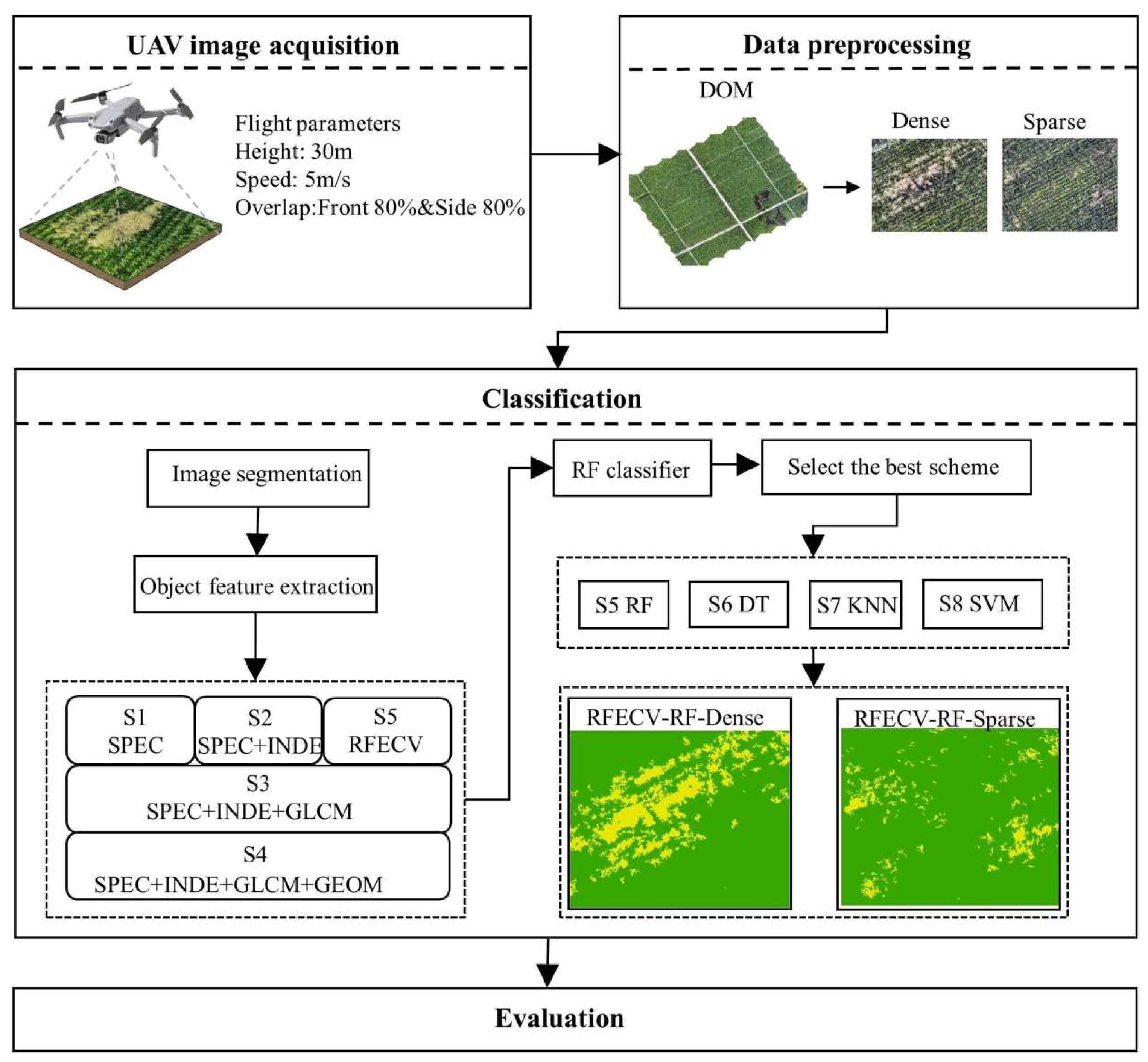
2.2. Method
2.2.1. Data Acquisition and Preprocessing
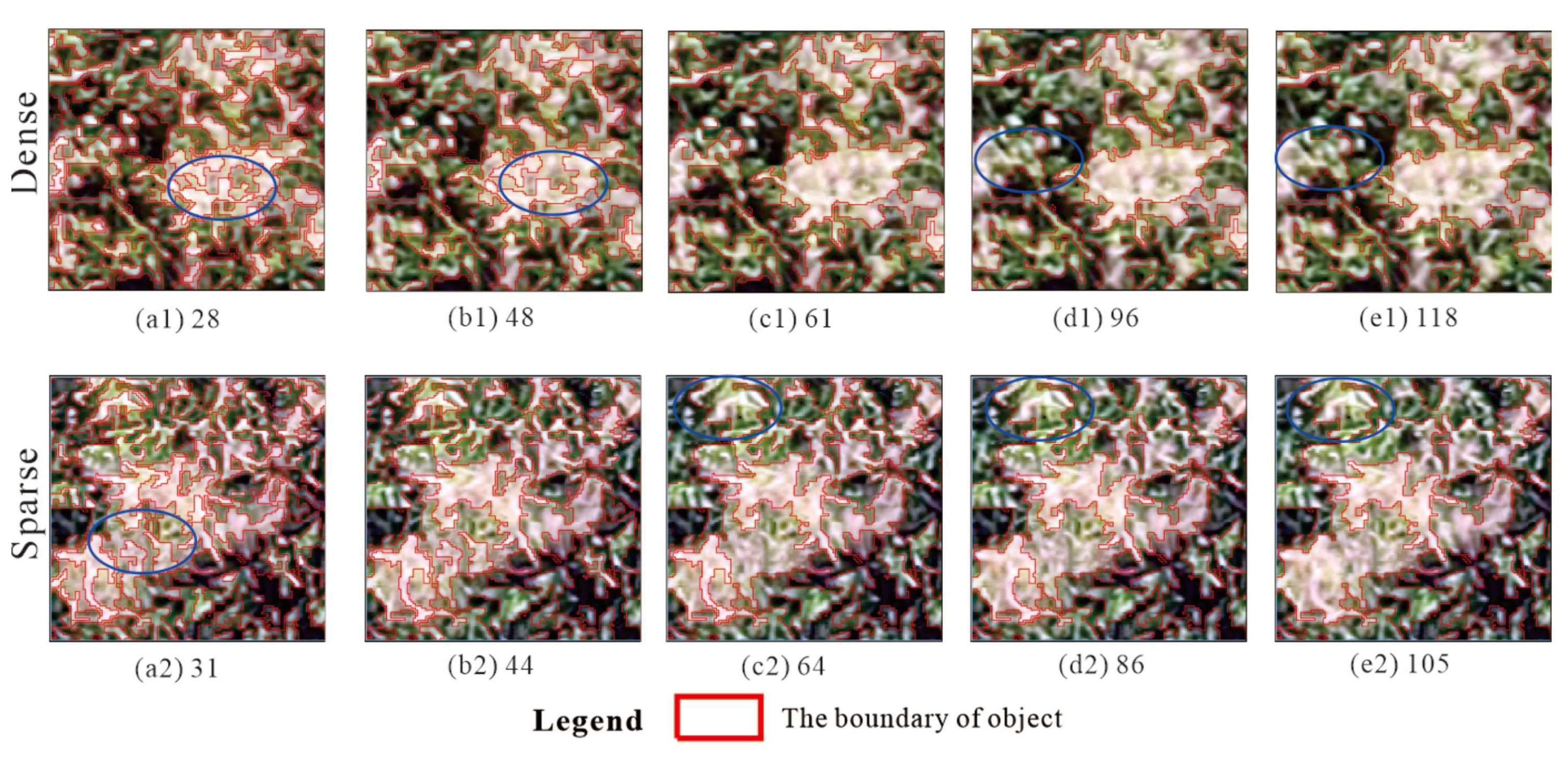
2.2.2. Image Segmentation
2.2.3. Feature Extraction
- (1)
- Spectral features (SPEC): The mean and standard deviation of three bands in the visible image (mean_R, mean_G, mean_B; Std_R, Std_G, Std_B), band maximum difference (Max_diff), and brightness [41];
- (2)
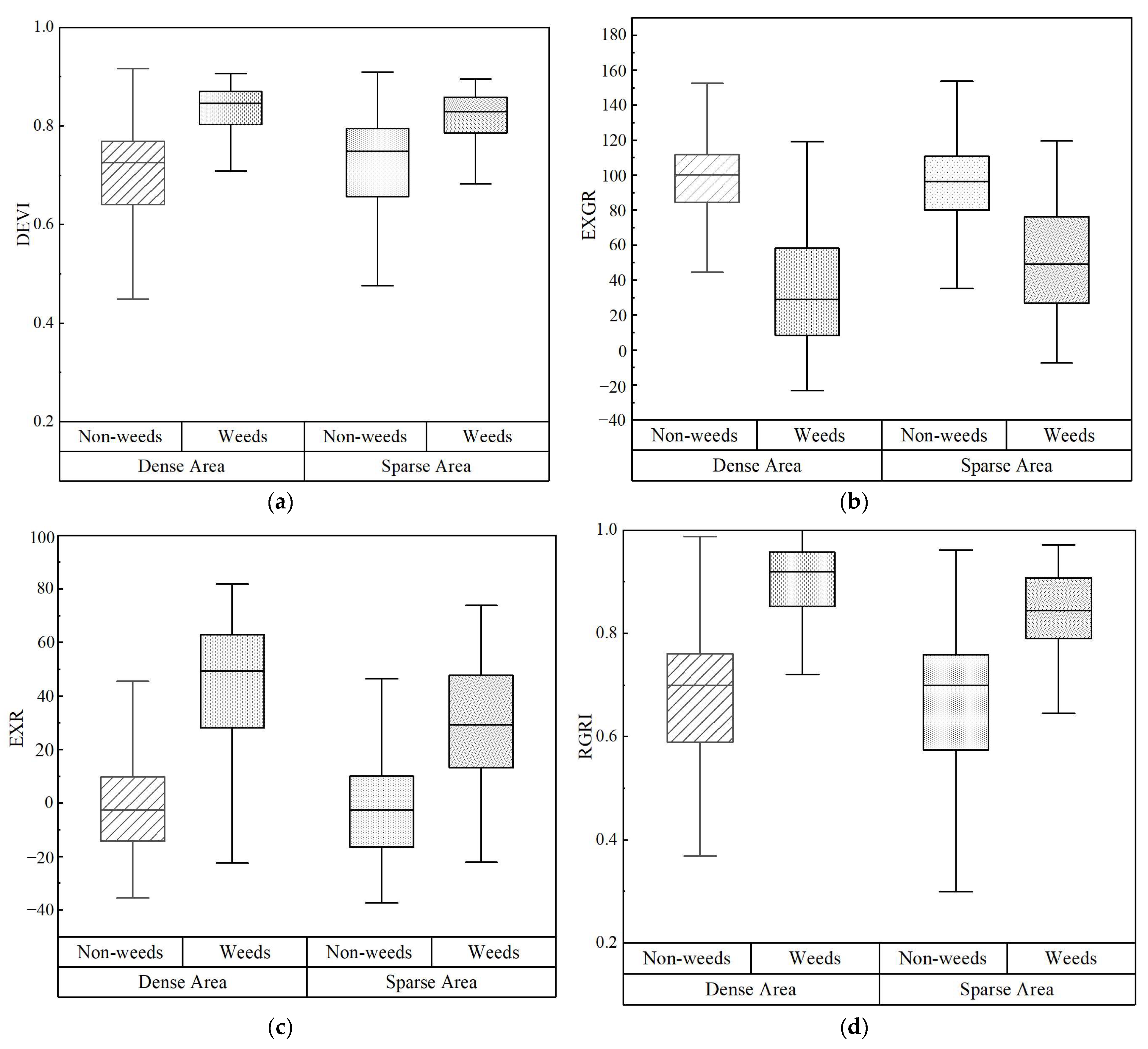
- Index features (INDE): Difference enhanced vegetation index (DEVI), excess red index (EXR), excess green index (EXG), excess green minus excess red (EXGR), green to blue ratio index (GBRI), greenness vegetation index (GVI), modified green-red vegetation index (MGRVI), normalized green-blue difference index (NGBDI), normalized green-red difference index (NGRDI), red-green-blue vegetation index (RGBVI), and visible-band difference vegetation index (VDVI). The vegetation indices and formulas are shown in Table 1;
- (3)
- Geometric features (GEOM): Area, length, length/width, width, border length, number of pixels, volume, asymmetry, border index, compactness, density, elliptic fit, shape, index, roundness, and rectangular fit [54];
- (4)
2.2.4. Sample Selection
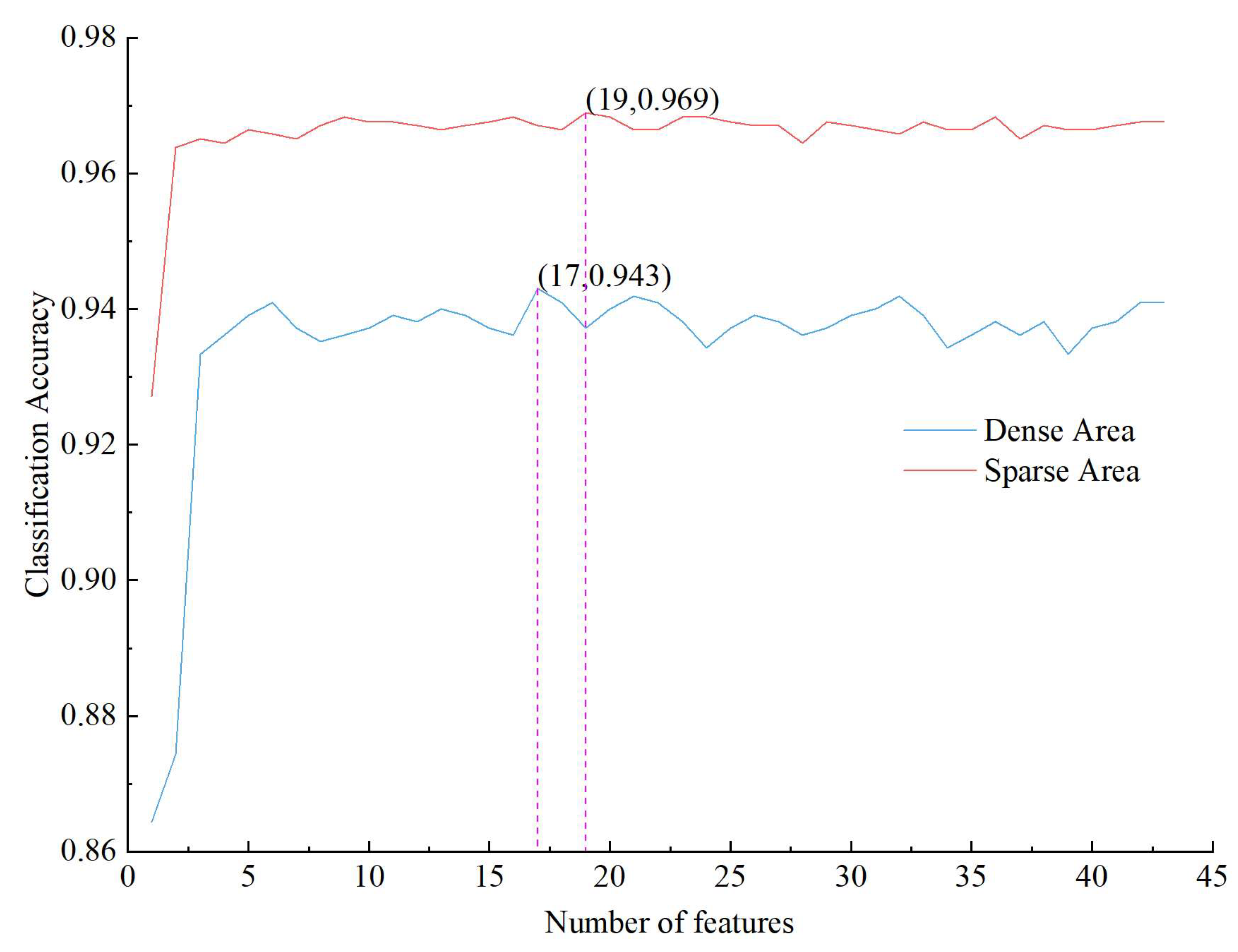
2.2.5. Feature Selection
2.2.6. Constructing the Experimental Scheme
2.2.7. Accuracy Evaluation Index
3. Results
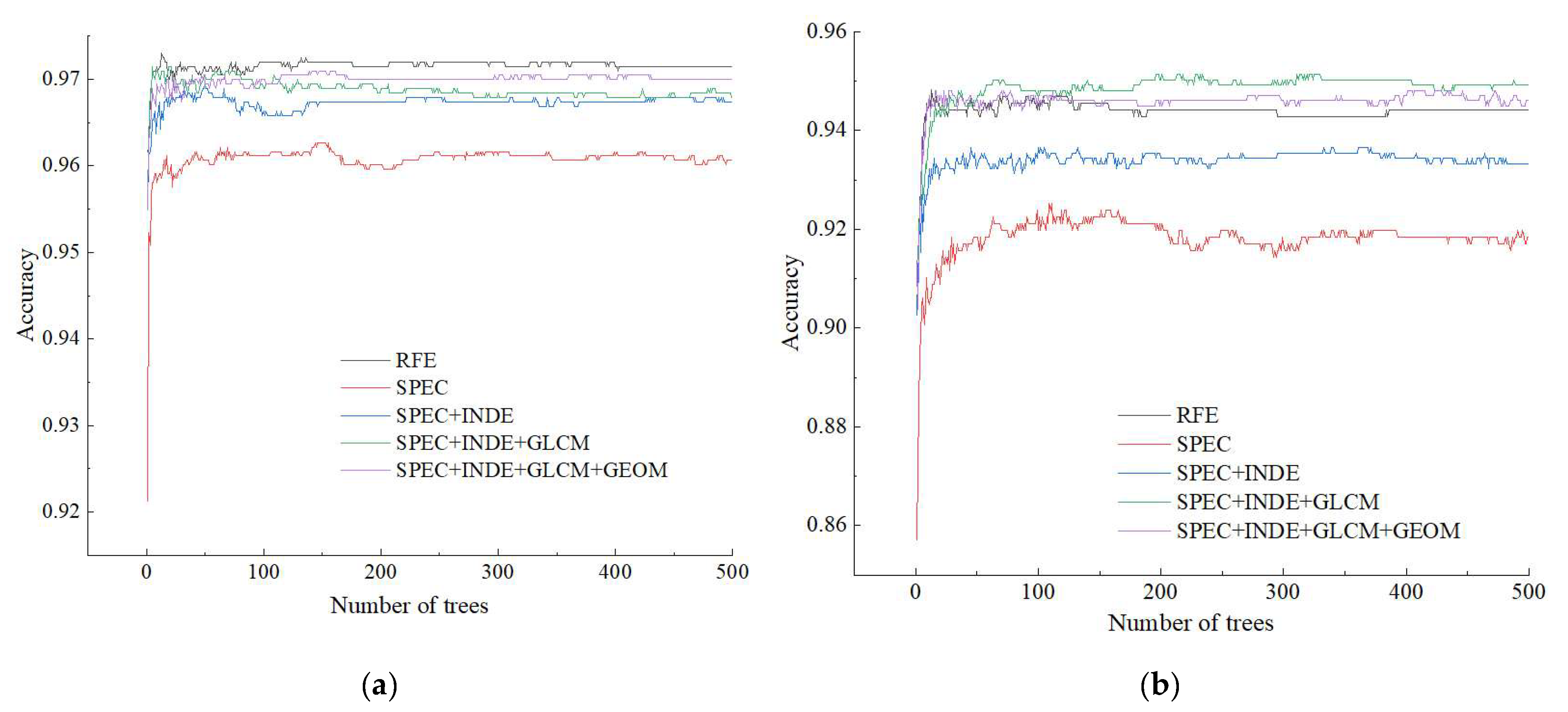
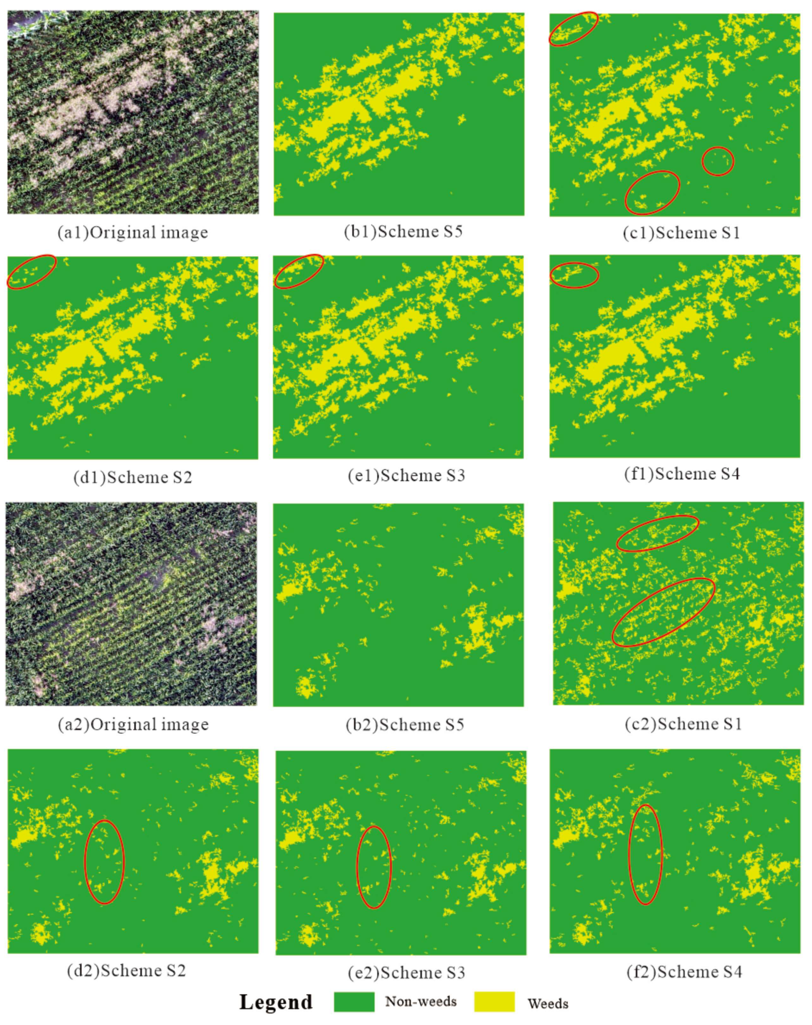
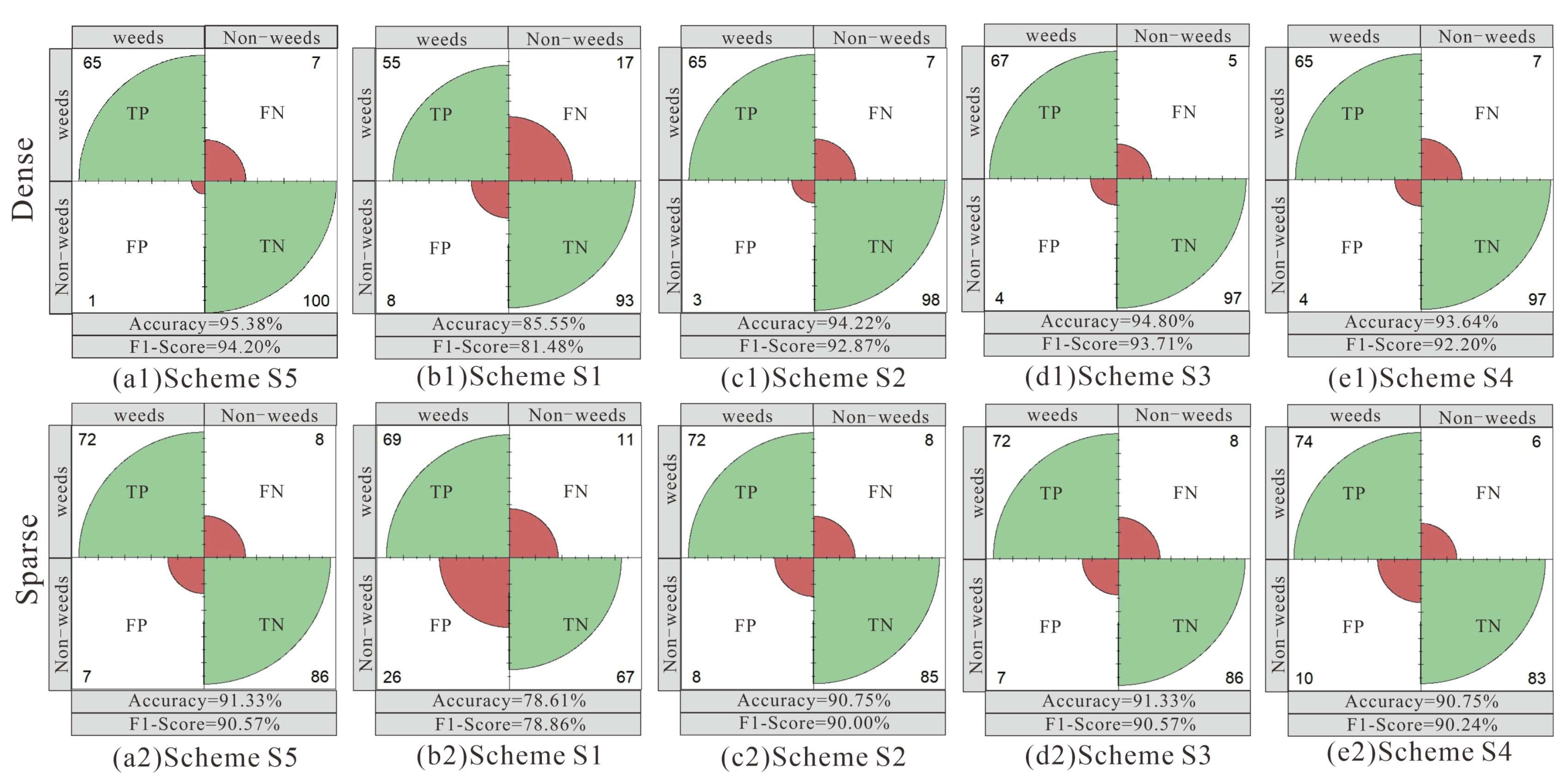
3.1. Results of the Different Feature Schemes
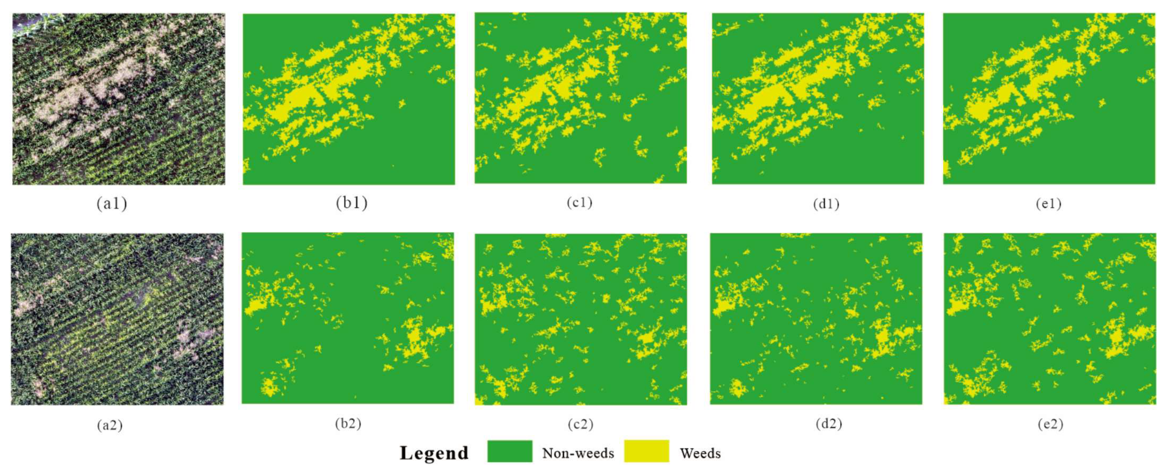
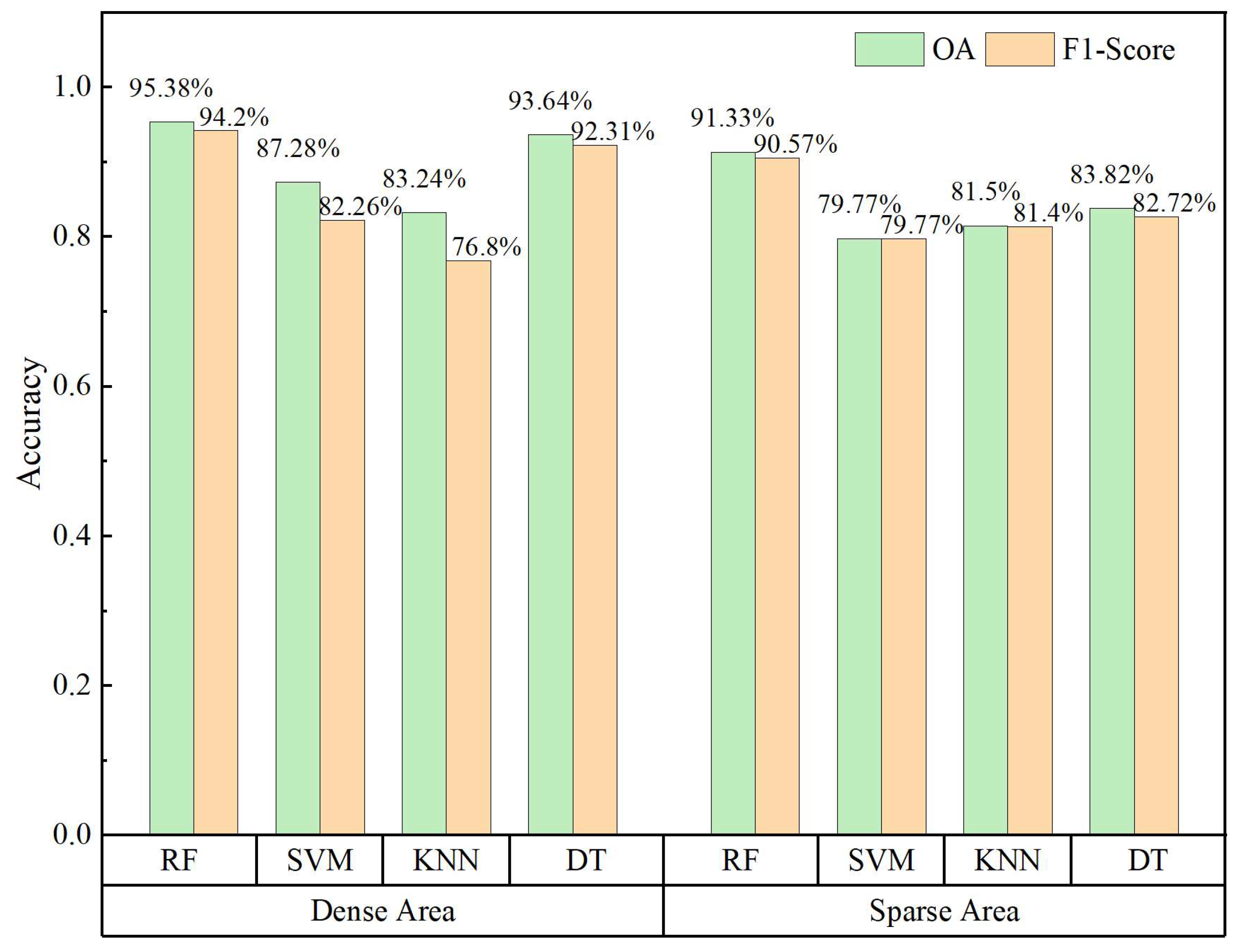
3.2. Results of the Different Machine Learning Algorithms
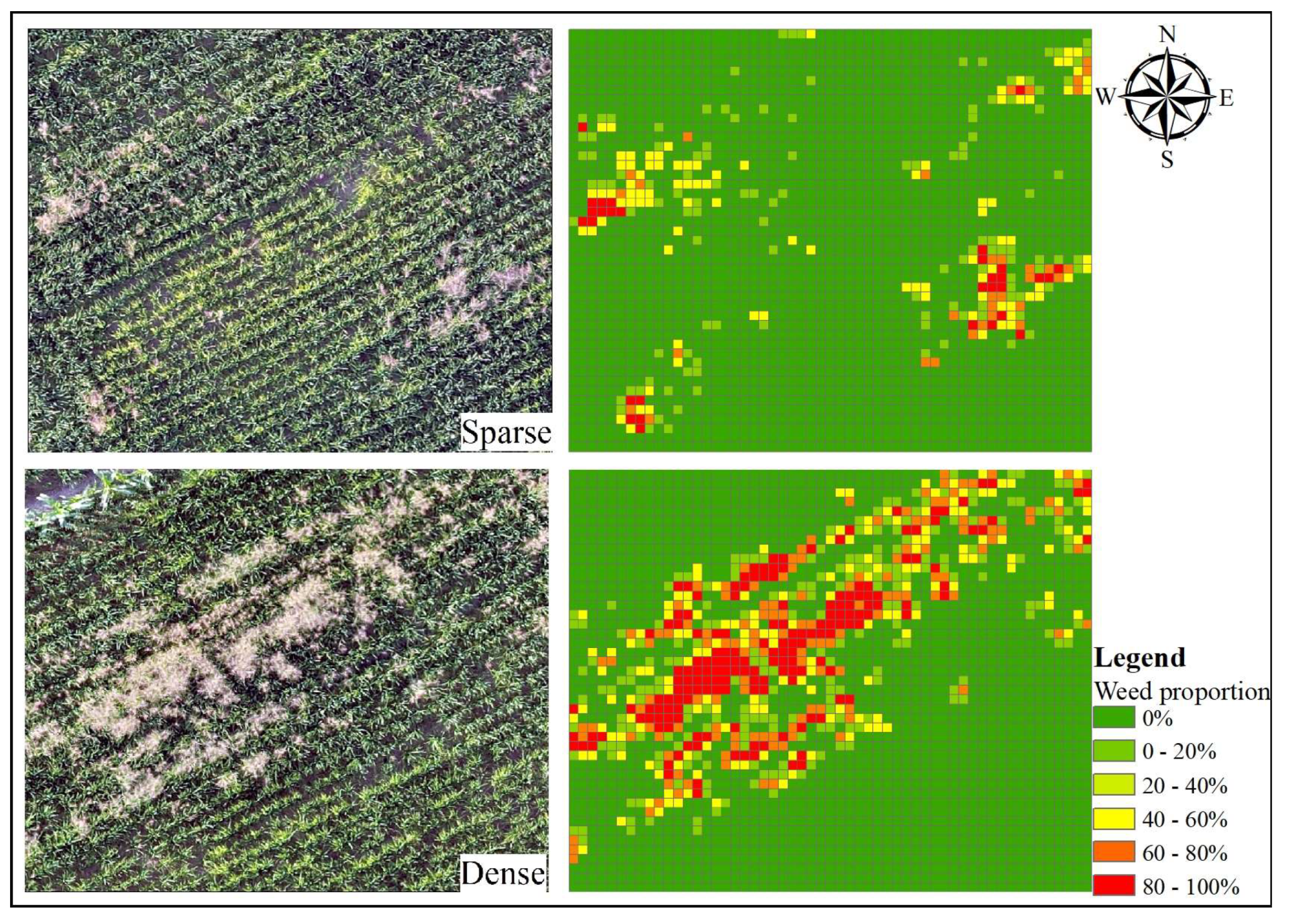
4. Application of Classification Results
5. Discussion
6. Conclusions
Author Contributions
Funding
Data Availability Statement
Acknowledgments
Conflicts of Interest
References
- Jin, X.; Liu, T.; McCullough, P.E.; Chen, Y.; Yu, J. Evaluation of convolutional neural networks for herbicide susceptibility-based weed detection in turf. Front. Plant Sci. 2023, 14, 1096802. [Google Scholar] [CrossRef] [PubMed]
- Zhang, X.; Cui, J.; Liu, H.; Han, Y.; Ai, H.; Dong, C.; Zhang, J.; Chu, Y. Weed Identification in Soybean Seedling Stage Based on Optimized Faster R-CNN Algorithm. Agriculture 2023, 13, 175. [Google Scholar] [CrossRef]
- Rawat, J.S.; Joshi, R.C. Remote-sensing and GIS-based landslide-susceptibility zonation using the landslide index method in Igo River Basin, Eastern Himalaya, India. Int. J. Remote Sens. 2012, 33, 3751–3767. [Google Scholar] [CrossRef]
- Zou, L.; Wang, C.; Zhang, H.; Wang, D.; Tang, Y.; Dai, H.; Zhang, B.; Wu, F.; Xu, L. Landslide-prone area retrieval and earthquake-inducing hazard probability assessment based on InSAR analysis. Landslides 2023, 20, 1989–2002. [Google Scholar] [CrossRef]
- Asadzadeh, S.; Oliveira, W.J.D.; Souza Filho, C.R.D. UAV-based remote sensing for the petroleum industry and environmental monitoring: State-of-the-art and perspectives. J. Pet. Sci. Eng. 2022, 208, 109633. [Google Scholar] [CrossRef]
- Yang, C.; Shen, R.; Yu, D.; Liu, R.; Chen, J. Forest disturbance monitoring based on the time-series trajectory of remote sensing index. J. Remote Sens. 2013, 17, 1246–1263. [Google Scholar] [CrossRef]
- He, X.Y.; Ren, C.Y.; Chen, L.; Wang, Z.; Zheng, H. The progress of forest ecosystems monitoring with remote sensing techniques. Sci. Geogr. Sin. 2018, 38, 997–1011. [Google Scholar] [CrossRef]
- Gao, F.; Anderson, M.; Daughtry, C.; Karnieli, A.; Hively, D.; Kustas, W. A within-season approach for detecting early growth stages in corn and soybean using high temporal and spatial resolution imagery. Remote Sens. Environ. 2020, 242, 111752. [Google Scholar] [CrossRef]
- Guilherme Teixeira Crusiol, L.; Sun, L.; Chen, R.; Sun, Z.; Zhang, D.; Chen, Z.; Wuyun, D.; Rafael Nanni, M.; Lima Nepomuceno, A.; Bouças Farias, J.R. Assessing the potential of using high spatial resolution daily NDVI-time-series from Planet CubeSat images for crop monitoring. Int. J. Remote Sens. 2021, 42, 7114–7142. [Google Scholar] [CrossRef]
- Lu, Y.; Chibarabada, T.P.; Ziliani, M.G.; Onema, J.K.; McCabe, M.F.; Sheffield, J. Assimilation of soil moisture and canopy cover data improves maize simulation using an under-calibrated crop model. Agric. Water Manag. 2021, 252, 106884. [Google Scholar] [CrossRef]
- Li, D.; Li, M. Research advance and application prospect of unmannedaerial vehicle remote sensing system. Geomat. Inf. Sci. Wuhan Univ. 2014, 39, 505–513. [Google Scholar] [CrossRef]
- Stroppiana, D.; Villa, P.; Sona, G.; Ronchetti, G.; Candiani, G.; Pepe, M.; Busetto, L.; Migliazzi, M.; Boschetti, M. Early season weed mapping in rice crops using multi-spectral UAV data. Int. J. Remote Sens. 2018, 39, 5432–5452. [Google Scholar] [CrossRef]
- Ye, Z.; Guo, Q.; Zhang, J.; Zhang, H.; Deng, H. Extraction of urban impervious surface based on the visible images of UAV and OBIA-RF algorithm. Trans. Chin. Soc. Agric. Eng. 2022, 38, 225–234. [Google Scholar] [CrossRef]
- Yonah, I.B.; Mourice, S.K.; Tumbo, S.D.; Mbilinyi, B.P.; Dempewolf, J. Unmanned aerial vehicle-based remote sensing in monitoring smallholder, heterogeneous crop fields in Tanzania. Int. J. Remote Sens. 2018, 39, 5453–5471. [Google Scholar] [CrossRef]
- Noguera, M.; Aquino, A.; Ponce, J.M.; Cordeiro, A.; Silvestre, J.; Arias-Calderón, R.; Da Encarnação Marcelo, M.; Jordão, P.; Andújar, J.M. Nutritional status assessment of olive crops by means of the analysis and modelling of multispectral images taken with UAVs. Biosyst. Eng. 2021, 211, 1–18. [Google Scholar] [CrossRef]
- Qin, Z.; Chang, Q.; Xie, B.; Shen, J. Rice leaf nitrogen content estimation based on hysperspectral imagery of UAV in Yellow River diversion irrigation district. Trans. Chin. Soc. Agric. Eng. 2016, 32, 77–85. [Google Scholar] [CrossRef]
- Atik, S.O.; Ipbuker, C. Integrating Convolutional Neural Network and Multiresolution Segmentation for Land Cover and Land Use Mapping Using Satellite Imagery. Appl. Sci. 2021, 11, 5551. [Google Scholar] [CrossRef]
- Guirado, E.; Blanco-Sacristán, J.; Rodríguez-Caballero, E.; Tabik, S.; Alcaraz-Segura, D.; Martínez-Valderrama, J.; Cabello, J. Mask R-CNN and OBIA Fusion Improves the Segmentation of Scattered Vegetation in Very High-Resolution Optical Sensors. Sensors 2021, 21, 320. [Google Scholar] [CrossRef]
- Ye, Z.; Yang, K.; Lin, Y.; Guo, S.; Sun, Y.; Chen, X.; Lai, R.; Zhang, H. A comparison between Pixel-based deep learning and Object-based image analysis (OBIA) for individual detection of cabbage plants based on UAV Visible-light images. Comput. Electron. Agric. 2023, 209, 107822. [Google Scholar] [CrossRef]
- Benz, U.C.; Hofmann, P.; Willhauck, G.; Lingenfelder, I.; Heynen, M. Multi-resolution, object-oriented fuzzy analysis of remote sensing data for GIS-ready information. ISPRS-J. Photogramm. Remote Sens. 2004, 58, 239–258. [Google Scholar] [CrossRef]
- Blaschke, T. Object based image analysis for remote sensing. ISPRS-J. Photogramm. Remote Sens. 2010, 65, 2–16. [Google Scholar] [CrossRef]
- Blaschke, T.; Hay, G.J.; Kelly, M.; Lang, S.; Hofmann, P.; Addink, E.; Feitosa, R.Q.; Van der Meer, F.; Van der Werff, H.; Van Coillie, F. Geographic object-based image analysis–towards a new paradigm. ISPRS-J. Photogramm. Remote Sens. 2014, 87, 180–191. [Google Scholar] [CrossRef]
- Liu, T.; Abd-Elrahman, A.; Zare, A.; Dewitt, B.A.; Flory, L.; Smith, S.E. A fully learnable context-driven object-based model for mapping land cover using multi-view data from unmanned aircraft systems. Remote Sens. Environ. 2018, 216, 328–344. [Google Scholar] [CrossRef]
- Tompalski, P.; White, J.C.; Coops, N.C.; Wulder, M.A. Demonstrating the transferability of forest inventory attribute models derived using airborne laser scanning data. Remote Sens. Environ. 2019, 227, 110–124. [Google Scholar] [CrossRef]
- Peña-Barragán, J.M.; Ngugi, M.K.; Plant, R.E.; Six, J. Object-based crop identification using multiple vegetation indices, textural features and crop phenology. Remote Sens. Environ. 2011, 115, 1301–1316. [Google Scholar] [CrossRef]
- Phiri, D.; Morgenroth, J.; Xu, C.; Hermosilla, T. Effects of pre-processing methods on Landsat OLI-8 land cover classification using OBIA and random forests classifier. Int. J. Appl. Earth Obs. Geoinf. 2018, 73, 170–178. [Google Scholar] [CrossRef]
- Bao, F.; Huang, K.; Wu, S. The retrieval of aerosol optical properties based on a random forest machine learning approach: Exploration of geostationary satellite images. Remote Sens. Environ. 2023, 286, 113426. [Google Scholar] [CrossRef]
- Loozen, Y.; Rebel, K.T.; de Jong, S.M.; Lu, M.; Ollinger, S.V.; Wassen, M.J.; Karssenberg, D. Mapping canopy nitrogen in European forests using remote sensing and environmental variables with the random forests method. Remote Sens. Environ. 2020, 247, 111933. [Google Scholar] [CrossRef]
- Wang, L.J.; Kong, Y.R.; Yang, X.D.; Xu, Y.; Liang, L.; Wang, S.G. Classification of land use in farming areas based on feature optimization random forest algorithm. Trans. CSAE 2020, 36, 244–250. [Google Scholar] [CrossRef]
- Yang, Y.; Zhang, W. Research on GF-2 Image Classification Based on Feature Optimization Random Forest Algorithm. Spacecr. Recovery Remote Sens. 2022, 43, 115–126. [Google Scholar] [CrossRef]
- Borra-Serrano, I.; Peña, J.M.; Torres-Sánchez, J.; Mesas-Carrascosa, F.J.; López-Granados, F. Spatial quality evaluation of resampled unmanned aerial vehicle-imagery for weed mapping. Sensors 2015, 15, 19688–19708. [Google Scholar] [CrossRef] [PubMed]
- Gao, J.; Liao, W.; Nuyttens, D.; Lootens, P.; Vangeyte, J.; Pižurica, A.; He, Y.; Pieters, J.G. Fusion of pixel and object-based features for weed mapping using unmanned aerial vehicle imagery. Int. J. Appl. Earth Obs. Geoinf. 2018, 67, 43–53. [Google Scholar] [CrossRef]
- Castillejo-González, I.L.; Peña-Barragán, J.M.; Jurado-Expósito, M.; Mesas-Carrascosa, F.J.; López-Granados, F. Evaluation of pixel- and object-based approaches for mapping wild oat (Avena sterilis) weed patches in wheat fields using QuickBird imagery for site-specific management. Eur. J. Agron. 2014, 59, 57–66. [Google Scholar] [CrossRef]
- Zhao, H.; Cao, Y.; Yue, Y.; Wang, H. Field weed recognition based on improved DenseNet. Trans. CSAE 2021, 37, 136–142. [Google Scholar] [CrossRef]
- Chen, J.; Wang, H.; Zhang, H.; Luo, T.; Wei, D.; Long, T.; Wang, Z. Weed detection in sesame fields using a YOLO model with an enhanced attention mechanism and feature fusion. Comput. Electron. Agric. 2022, 202, 107412. [Google Scholar] [CrossRef]
- Wang, C.; Wu, X.; Zhang, Y.; Wang, W. Recognizing weeds in maize fields using shifted window Transformer network. Trans. Chin. Soc. Agric. Eng. 2022, 38, 133–142. [Google Scholar] [CrossRef]
- Rana, M.; Kharel, S. FEATURe Extraction for Urban and Agricultural Domains Using Ecognition Developer. Int. Arch. Photogramm. Remote Sens. Spat. Inf. Sci. 2019, XLII-3/W6, 609–615. [Google Scholar] [CrossRef]
- Sheng, R.T.; Huang, Y.; Chan, P.; Bhat, S.A.; Wu, Y.; Huang, N. Rice Growth Stage Classification via RF-Based Machine Learning and Image Processing. Agriculture 2022, 12, 2137. [Google Scholar] [CrossRef]
- Lagogiannis, S.; Dimitriou, E. Discharge Estimation with the Use of Unmanned Aerial Vehicles (UAVs) and Hydraulic Methods in Shallow Rivers. Water 2021, 13, 2808. [Google Scholar] [CrossRef]
- Yu, H.; Zhang, S.Q.; Kong, B.; Li, X. Optimal segmentation scale selection for object-oriented remote sensing image classification. J. Image Graph. 2010, 15, 352–360. [Google Scholar]
- Tian, J.; Wang, L.; Yin, D.; Li, X.; Diao, C.; Gong, H.; Shi, C.; Menenti, M.; Ge, Y.; Nie, S.; et al. Development of spectral-phenological features for deep learning to understand Spartina alterniflora invasion. Remote Sens. Environ. 2020, 242, 111745. [Google Scholar] [CrossRef]
- Zhou, T.; Hu, Z.; Han, J.; Zhang, H. Green vegetation extraction based on visible light image of UAV. China Environ. Sci. 2021, 41, 2380–2390. [Google Scholar] [CrossRef]
- Sánchez-Sastre, L.F.; Alte Da Veiga, N.M.; Ruiz-Potosme, N.M.; Carrión-Prieto, P.; Marcos-Robles, J.L.; Navas-Gracia, L.M.; Martín-Ramos, P. Assessment of RGB vegetation indices to estimate chlorophyll content in sugar beet leaves in the final cultivation stage. AgriEngineering 2020, 2, 128–149. [Google Scholar] [CrossRef]
- Yang, B.; Wang, M.; Sha, Z.; Wang, B.; Chen, J.; Yao, X.; Cheng, T.; Cao, W.; Zhu, Y. Evaluation of aboveground nitrogen content of winter wheat using digital imagery of unmanned aerial vehicles. Sensors 2019, 19, 4416. [Google Scholar] [CrossRef] [PubMed]
- Jiang, J.; Zhang, Z.; Cao, Q.; Tian, Y.; Zhu, Y.; Cao, W.; Liu, X. Use of a digital camera mounted on a consumer-grade unmanned aerial vehicle to monitor the growth status of wheat. J. Nanjing Agric. Univ. 2019, 42, 622–631. [Google Scholar] [CrossRef]
- Sellaro, R.; Crepy, M.; Trupkin, S.A.; Karayekov, E.; Buchovsky, A.S.; Rossi, C.; Casal, J.J. Cryptochrome as a sensor of the blue/green ratio of natural radiation in Arabidopsis. Plant Physiol. 2010, 154, 401–409. [Google Scholar] [CrossRef]
- Liu, Y.; Chen, Y.; Yue, D.; Feng, Z. Information extraction of urban green space based on UAV remote sensing image. Sci. Surv. Mapp. 2017, 42, 59–64. [Google Scholar] [CrossRef]
- Bendig, J.; Yu, K.; Aasen, H.; Bolten, A.; Bennertz, S.; Broscheit, J.; Gnyp, M.L.; Bareth, G. Combining UAV-based plant height from crop surface models, visible, and near infrared vegetation indices for biomass monitoring in barley. Int. J. Appl. Earth Obs. Geoinf. 2015, 39, 79–87. [Google Scholar] [CrossRef]
- Zhao, J.; Yang, H.B.; Lan, Y.B.; Lu, L.Q.; Jia, P.; Li, Z.M. Extraction method of summer corn vegetation coverage based on visible light image of unmanned aerial vehicle. J. Agric. Mach. 2019, 50, 232–240. [Google Scholar] [CrossRef]
- Elazab, A.; Bort, J.; Zhou, B.; Serret, M.D.; Nieto-Taladriz, M.T.; Araus, J.L. The combined use of vegetation indices and stable isotopes to predict durum wheat grain yield under contrasting water conditions. Agric. Water Manag. 2015, 158, 196–208. [Google Scholar] [CrossRef]
- Li, C.C.; Niu, Q.L.; Yang, G.J.; Feng, H.; Liu, J.; Wang, Y. Estimation of leaf area index of soybean breeding materials based on UAV digital images. Trans. Chin. Soc. Agric. Mach. 2017, 48, 147. [Google Scholar] [CrossRef]
- Gamon, J.A.; Surfus, J.S. Assessing leaf pigment content and activity with a reflectometer. New Phytol. 1999, 143, 105–117. [Google Scholar] [CrossRef]
- Wang, X.; Wang, M.; Wang, S.; Wu, Y. Extraction of vegetation information from visible unmanned aerial vehicle images. Trans. Chin. Soc. Agric. Eng. 2015, 31, 152–159. [Google Scholar] [CrossRef]
- Yu, N.; Li, L.; Schmitz, N.; Tian, L.F.; Greenberg, J.A.; Diers, B.W. Development of methods to improve soybean yield estimation and predict plant maturity with an unmanned aerial vehicle based platform. Remote Sens. Environ. 2016, 187, 91–101. [Google Scholar] [CrossRef]
- Batool, F.E.; Attique, M.; Sharif, M.; Javed, K.; Nazir, M.; Abbasi, A.A.; Iqbal, Z.; Riaz, N. Offline signature verification system: A novel technique of fusion of GLCM and geometric features using SVM. Multimed. Tools Appl. 2020. [Google Scholar] [CrossRef]
- Mirzahossein, H.; Sedghi, M.; Motevalli Habibi, H.; Jalali, F. Site selection methodology for emergency centers in Silk Road based on compatibility with Asian Highway network using the AHP and ArcGIS (case study: I. R. Iran). Innov. Infrastruct. Solut. 2020, 5, 113. [Google Scholar] [CrossRef]
- Lin, X.; Yang, F.; Zhou, L.; Yin, P.; Kong, H.; Xing, W.; Lu, X.; Jia, L.; Wang, Q.; Xu, G. A support vector machine-recursive feature elimination feature selection method based on artificial contrast variables and mutual information. J. Chromatogr. B 2012, 910, 149–155. [Google Scholar] [CrossRef]
- Soper, D.S. Greed Is Good: Rapid Hyperparameter Optimization and Model Selection Using Greedy k-Fold Cross Validation. Electronics 2021, 10, 1973. [Google Scholar] [CrossRef]
- Alcantara, L.M.; Schenkel, F.S.; Lynch, C.; Oliveira Junior, G.A.; Baes, C.F.; Tulpan, D. Machine learning classification of breeding protocol descriptions from Canadian Holsteins. J. Dairy Sci. 2022, 105, 8177–8188. [Google Scholar] [CrossRef]
- Ye, S.; Pontius, R.G.; Rakshit, R. A review of accuracy assessment for object-based image analysis: From per-pixel to per-polygon approaches. ISPRS-J. Photogramm. Remote Sens. 2018, 141, 137–147. [Google Scholar] [CrossRef]
- Li, Z.; Ding, J.; Zhang, H.; Feng, Y. Classifying individual shrub species in UAV images-a case study of the gobi region of Northwest China. Remote Sens. 2021, 13, 4995. [Google Scholar] [CrossRef]
- Anderson, C.J.; Heins, D.; Pelletier, K.C.; Knight, J.F. Improving Machine Learning Classifications of Phragmites australis Using Object-Based Image Analysis. Remote Sens. 2023, 15, 989. [Google Scholar] [CrossRef]
- Pena, J.M.; Torres-Sanchez, J.; de Castro, A.I.; Kelly, M.; Lopez-Granados, F. Weed mapping in early-season maize fields using object-based analysis of unmanned aerial vehicle (UAV) images. PLoS ONE 2013, 8, e77151. [Google Scholar] [CrossRef] [PubMed]
- Jing, X.; Zou, Q.; Yan, J.; Dong, Y.; Li, B. Remote Sensing Monitoring of Winter Wheat Stripe Rust Based on mRMR-XGBoost Algorithm. Remote Sens. 2022, 14, 756. [Google Scholar] [CrossRef]
- Li, H.; Cui, J.; Zhang, X.; Han, Y.; Cao, L. Dimensionality Reduction and Classification of Hyperspectral Remote Sensing Image Feature Extraction. Remote Sens. 2022, 14, 4579. [Google Scholar] [CrossRef]
- Bhagwat, R.U.; Uma Shankar, B. A novel multilabel classification of remote sensing images using XGBoost. In Proceedings of the 2019 IEEE 5th International Conference for Convergence in Technology (I2CT), Bombay, India, 29–31 March 2019; pp. 1–5. [Google Scholar] [CrossRef]
- Han, L.; Yang, G.; Yang, X.; Song, X.; Xu, B.; Li, Z.; Wu, J.; Yang, H.; Wu, J. An explainable XGBoost model improved by SMOTE-ENN technique for maize lodging detection based on multi-source unmanned aerial vehicle images. Comput. Electron. Agric. 2022, 194, 106804. [Google Scholar] [CrossRef]


| Vegetation Index | Formulas | Reference |
|---|---|---|
| DEVI | [42] | |
| EXG | [43] | |
| EXGR | [44] | |
| EXR | [45] | |
| GBRI | [46] | |
| GVI | [47] | |
| MGRVI | [48] | |
| NGBDI | [49] | |
| NGRDI | [50] | |
| RGBVI | [51] | |
| RGRI | [52] | |
| VDVI | [53] |
| Texture Feature | Formulas |
|---|---|
| Mean | |
| Standard Deviation | |
| Entropy | |
| Homogeneity | |
| Dissimilarity | |
| Contract | |
| Correlation | |
| Angular Second Moment |
| Scheme | Classifier | Features | Number of Features (Sparse/Dense) | Number of Trees (Sparse/Dense) |
|---|---|---|---|---|
| S1 | Random Forest | SPEC | 8/8 | 135/105 |
| S2 | Random Forest | SPEC + INDE | 20/20 | 65/106 |
| S3 | Random Forest | SPEC + INDE + GLCM | 28/28 | 9/175 |
| S4 | Random Forest | SPEC + INDE + GLCM + GEOM | 43/43 | 125/121 |
| S5 | Random Forest | RFECV | 19/17 | 26/26 |
| S6 | SVM | RFECV | 19/17 | — |
| S7 | Decision Tree | RFECV | 19/17 | — |
| S8 | KNN | RFECV | 19/17 | — |
Disclaimer/Publisher’s Note: The statements, opinions and data contained in all publications are solely those of the individual author(s) and contributor(s) and not of MDPI and/or the editor(s). MDPI and/or the editor(s) disclaim responsibility for any injury to people or property resulting from any ideas, methods, instructions or products referred to in the content. |
© 2023 by the authors. Licensee MDPI, Basel, Switzerland. This article is an open access article distributed under the terms and conditions of the Creative Commons Attribution (CC BY) license (https://creativecommons.org/licenses/by/4.0/).
Share and Cite
Feng, C.; Zhang, W.; Deng, H.; Dong, L.; Zhang, H.; Tang, L.; Zheng, Y.; Zhao, Z. A Combination of OBIA and Random Forest Based on Visible UAV Remote Sensing for Accurately Extracted Information about Weeds in Areas with Different Weed Densities in Farmland. Remote Sens. 2023, 15, 4696. https://doi.org/10.3390/rs15194696
Feng C, Zhang W, Deng H, Dong L, Zhang H, Tang L, Zheng Y, Zhao Z. A Combination of OBIA and Random Forest Based on Visible UAV Remote Sensing for Accurately Extracted Information about Weeds in Areas with Different Weed Densities in Farmland. Remote Sensing. 2023; 15(19):4696. https://doi.org/10.3390/rs15194696
Chicago/Turabian StyleFeng, Chao, Wenjiang Zhang, Hui Deng, Lei Dong, Houxi Zhang, Ling Tang, Yu Zheng, and Zihan Zhao. 2023. "A Combination of OBIA and Random Forest Based on Visible UAV Remote Sensing for Accurately Extracted Information about Weeds in Areas with Different Weed Densities in Farmland" Remote Sensing 15, no. 19: 4696. https://doi.org/10.3390/rs15194696
APA StyleFeng, C., Zhang, W., Deng, H., Dong, L., Zhang, H., Tang, L., Zheng, Y., & Zhao, Z. (2023). A Combination of OBIA and Random Forest Based on Visible UAV Remote Sensing for Accurately Extracted Information about Weeds in Areas with Different Weed Densities in Farmland. Remote Sensing, 15(19), 4696. https://doi.org/10.3390/rs15194696