Research on UT1-UTC and LOD Prediction Algorithm Based on Denoised EAM Dataset

Abstract

The components of EAM are strongly correlated with LOD and play an important role in UT1-UTC and LOD prediction. However, the EAM dataset is prone to be noisy. In this study, we propose a hybrid method to reduce the noise of the EAM data and improve the accuracy of UT1-UTC and LOD predictions. We use the EOP data to denoise the EAM data, and use Kalman filtering to denoise the 1–6 days forecast of EAM. Then, we use the denoised EAM dataset to improve the UT1-UTC and LOD prediction. The denoised EAM dataset improved the prediction of UT1-UTC within 10 days by 20%. In addition, we found that by introducing two additional periodic (23.9 days and 91.3 days) components for the least-squares fitting, the accuracy of UT1-UTC and LOD prediction in the range of 30–80 days is significantly improved. In more than 430 UT1-UTC and LOD prediction experiments conducted during 2021–2022, the improvements in the 1–6 days forecast were significant. For the 6th day, 30th day, and 60th day, the MAE of UT1-UTC was 0.1592, 2.9169, and 6.7857 ms, respectively, corresponding to improvements of 31.35, 12.60, and 12.93%, respectively, when compared to predictions of Bulletin A. The MAE of LOD predictions on the 1st day, 6th day, 30th day, and 90th day was 0.0255, 0.0432, 0.1694, and 0.2505 ms, respectively, which improved by 26.09, 14.29, 6.36, and 3.76% when compared with our second EOPPCC method.

1. Introduction

Universal time (UT1) is a time scale defined by the Earth’s rotation, which describes the rotation angle of the solid Earth around its instantaneous rotation axis in the ‘’inertial’’ celestial reference frame. The Length of Day (LOD) measures the variations in the Earth’s rotation rate and reflects the speed of Earth’s rotation. UT1, LOD, polar motion (PM), nutation, and precession constitute a set of parameters called Earth Orientation Parameters (EOP), which describe the spin of the Earth about its rotation axis, and orientation of the rotation axis in the terrestrial and celestial reference frame. EOP are essential parameters for transforming coordinates between the celestial reference frame and the Earth reference frame, and play a crucial role in deep space exploration, satellite navigation, astrometry, geodynamics, and maintenance of the terrestrial reference frame (TRF) [1,2,3,4,5].

Accurate EOP can be measured from space-geodetic techniques such as Very Long Baseline Interferometry (VLBI) [6,7,8,9], Global Navigation Satellite System (GNSS) [10,11,12,13], Satellite Laser Ranging (SLR) [14], Lunar Laser Ranging (LLR) [15,16], and Doppler Orbitography and Radiopositioning Integrated by Satellite (DORIS) [17,18,19]. However, the determination of EOP is often delayed by several days or even weeks due to the large volume of observation data, and complex data processing procedures. For instance, GNSS technology typically introduces a delay of 4–6 h before EOP data can be obtained, while VLBI and SLR may require a delay of 2–5 days. The final products released by the International Earth Rotation Service (IERS), which integrates data from multiple space geodesy techniques, have a latency of around one month. To meet the real-time requirements of users, it is necessary to predict future EOP based on rapid solutions obtained from geodetic measurements [20,21,22,23].

Dozens of methods and algorithms for predictions of EOP have been proposed and explored, including (a) Spectral analysis combined with the least-squares extrapolation (LS) [24,25,26], (b) LS combined with autoregressive (AR) prediction [27,28], (c) Artificial neural networks (ANN) [5,29,30], (d) Wavelet decomposition (WD) combined with autocovariance prediction (AC) [31,32], (e) Kalman filter with atmospheric angular momentum (AAM) forecasts [33,34], (f) Adaptive transformation from AAM to LOD change [4], (g) LS combined with AR and Kalman filtering [35], (h) 6-day effective angular momentum (EAM) combined with LS and AR [36], and (i) Polynomial curve fitting (PCF) combined with weighted least squares (WLS) and AR [37].

The first comprehensive assessment of EOP prediction capabilities was carried out in the first EOP Prediction Comparison Campaign (1st EOP PCC) conducted by Vienna University of Technology and Centrum Badan Kosmicznych Polskiej Akademii Nauk (CBK PAN) between 2005 and 2009 [4]. For seasonal predictions, a combination of least-squares estimation and autoregressive modeling (LS + AR) was found to be the most reliable method. For short-term prediction horizons, the incorporation of Atmospheric Angular Momentum (AAM) forecasts into the prediction, particularly using a Kalman filter, resulted in significantly more accurate predictions compared to other methods [36].

The second EOP PCC campaign, coordinated by CBK PAN with support from the German Research Centre for Geosciences (GFZ), emerged as an international initiative involving 28 registered institutions from 9 different countries, with over 60 participants regularly providing predictions based on 56 different methods [38]. Tomasz et al. [38] analyzed the data collected during the period from 1 September 2021 to 29 May 2022, and found that using both observed and forecasted values of EAM for EOP prediction was effective. Nine months after the start of the second campaign, the Mean Absolute Error (MAE) for the 10th day of the UT1-UTC forecast ranged from 0.36 to 3.13 ms, while for the LOD forecast, it ranged from 0.07 to 0.28 ms. The results of the first campaign showed that the MAE for the 10th day of the UT1-UTC forecast ranged from 0.60 to 1.40 ms, and for the LOD forecast, it ranged from 0.13 to 0.40 ms, indicating significant progress in EOP forecasting in recent years [4,38].

The EAM + LS + AR forecasting method used in this paper is developed from the forecasting algorithm proposed by Dill et al. [36]. In the 2nd EOPPCC, we used a piecewise parameterization to optimize the parameters of LS and AR [39]. In this paper, we further improve the forecasting algorithm at two points: (a) The setting of LS fitting periodic terms. By analyzing the EAM, Geodetic Angular Momentum Functions (GAM), and the spectra of GAM-EAM, two strong periodic terms of 91.3 days and 23.9 days were identified and used, which were not used in Dill et al. [36]. By comparing the presence or absence of these two periodic terms, it was found that using the 23.9 days and 91.3 days periodic terms significantly improves the UT1-UTC and LOD forecast accuracy for the 30–80 days range. (b) Noise suppression of the EAM dataset, including the observed dataset and 1–6 day forecast dataset. Through comparing experiments with and without EAM noise suppression, it was found that EAM with noise suppression significantly improved the prediction accuracy of UT1-UTC and LOD within the range of 1–90 days, especially in the short-term forecast accuracy of 1–6 days. The Section 2 introduces the characteristics of the forecast dataset and the forecasting method, including the analysis of LS periodic terms, reconstruction of the EAM dataset, Kalman residual filtering, settings of forecasting parameters, and the forecasting process. The Section 3 presents the evaluation and comparison of different forecasting schemes. The Section 4 discusses the analysis and future prospects. A summary is given in the Section 5.

2. Materials and Methods

2.1. Dataset Analysis

The EAM function is composed of AAM, Oceanic Angular Momentum (OAM), Hydrological Angular Momentum (HAM), and Sea-level Angular effective Momentum (SLAM). The modeling process of OAM is extensively described in Jungclaus et al. [40], while Dill [41] outlines the calculation method for HAM. For more detailed information on AAM, SLAM, and other related concepts, please refer to Dobslaw and Dill [42,43], Tamisieaetal [44], Hageman and Dumenil [45]. The datasets for AAM, OAM, HAM, SLAM, and others can be downloaded from the Earth System Modelling Group of GFZ Potsdam (ESMGFZ) at the following website: http://esmdata.gfz-potsdam.de:8080 (accessed on 12 August 2023).

Using the empirical model provided by the IERS protocol, the IERS C04 LOD series was used to correct 62 solid Earth tidal harmonics with periods ranging from 5 days to 18.6 years [46]. After subtracting the solid tide harmonics, the LODR sequence (1a = 365.24d) was obtained. Using the Liouville equation [47], the LODR was then transformed into GAM.

$$\Psi =-\frac{\Omega }{2\pi }LODR$$

(1)

where $\Psi$ is the angular momentum function GAM, and $\Omega$ is the average angular velocity of the earth 7.292115 × 10⁻⁵ rad s⁻¹.

From Figure 1, it can be seen that EAM and GAM exhibit a high correlation (Pearson coefficient of 72.85%). Starting from 2020, the difference between the two series decreases, and both EAM and GAM display noticeable periodic components.

From the left panel of Figure 2, strong periodic features with periods of 182.60 and 365.25 days, as well as relatively weak features with periods of 91.30 and 121.74 days, are identified. From the right panel of Figure 2, strong features with periods of 9.13, 13.7, and 23.9 days are identified. It is noted that most of the periodic amplitudes of GAM-EAM are significantly lower than those of GAM. This indicates that EAM and GAM have a relatively consistent periodicity, and the EAM calculated based on the geophysical model is sufficient to explain most of the periodic signals. However, there is a lack of strong periodic components with periods of 9.13 and 13.7 days in EAM for short-period signals. Ray and Erofeeva [48] found residual tidal energy that is not reduced by the IERS tidal model for lunar tides at 18.6 and 9.3 years, solar tides at 365.25 and 182.6 days, as well as fortnightly Mf components with 13.7 days and Mt with 9.1 days, among others. Therefore, GAM, and consequently the GAM-EAM, still contain tidal contributions. It is worth mentioning that Dill et al. [36] observed a periodic component of 23.9 days in the spectral analysis but did not find a component with a period of 91.3 days. This discrepancy may be related to the length of the data used. However, Dill did not consider the components with periods of 23.9 and 91.3 days in the least-squares fitting. To validate the 23.9 and 91.3 days components, further prediction experiments were conducted to investigate the effects of these two periodic components.

2.2. The Denoised EAM Dataset

The EAM dataset plays an important role in UT1-UTC and LOD prediction [36,38,39]. However, the EAM dataset does not provide uncertainties for its data, including AAM, OAM, HAM, SLAM, and other raw data. Therefore, the accuracy of the EAM dataset is yet to be evaluated. The IERS C04 dataset, on the other hand, is a composite dataset obtained from various space geodetic measurement techniques and is currently the most accurate dataset of EOP. In this paper, a method is proposed to denoise the EAM dataset using the IERS C04 dataset. The aim is to suppress noise without changing the original characteristics of the EAM dataset. Firstly, a least-squares fitting is performed on the EAM and GAM datasets. Then, the least-squares fitting terms of the EAM dataset are combined with the least-squares residual of the GAM dataset to reconstruct a new EAM sequence. Utilizing the IERS C04 dataset and applying the proposed method is expected to improve the accuracy of the EAM dataset while preserving its inherent information. The least-squares formula is as follows:

$$f(t)=a_0+a_{1}t+\underset{i=1}{\overset{n}{\Sigma }}\left[c_i\sin (\frac{2\pi t}{T_i})+d_i\cos (\frac{2\pi t}{T_i})\right]$$

(2)

In the given formula, $a_0$ and $a_1$ represent the parameters of the linear trend component, $c_i$ and $d_i$ represent the parameters of the periodic component, $T_i$ represents the length of the periodic cycle, and $n$ represents the number of cycles. Here, $n$ is set to 10, and the values of $T_i$ correspond to 9.13, 13.7, 23.9, 27.4, 91.3, 121.75, 182.62, 365.24, 1095.72, and 3396.73 days. The settings for the periodic component are based on the spectral analysis in Section 2.1 and Dill et al. [36].

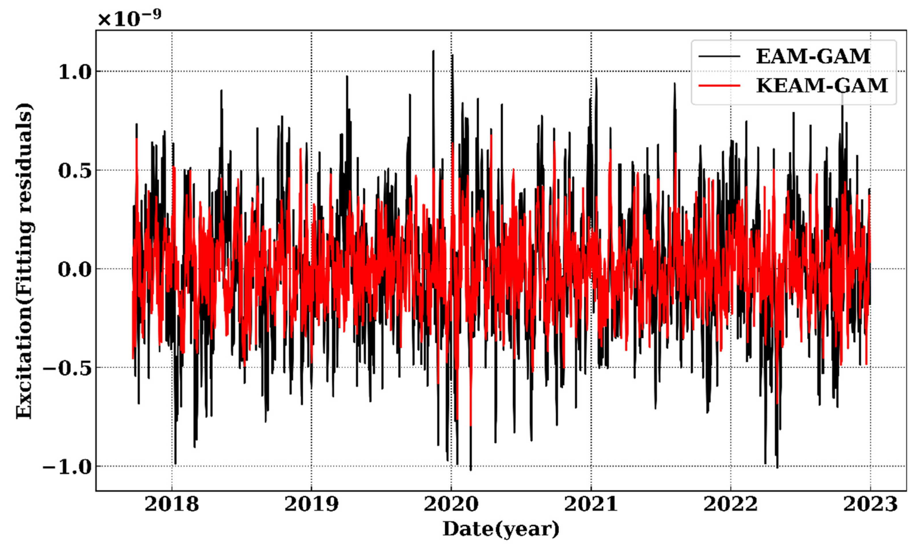
From Figure 3, it can be observed that the LS fitting residual of GAM and EAM exhibit a strong correlation, with similar magnitude fluctuations. The calculated Pearson coefficient reaches as high as 98.59%.

From Figure 4, it can be observed that the difference between the new EAM and the GAM, which preserves the same long-term trend and with much lower random fluctuations.

The 1–6 days forecast of the EAM dataset plays a crucial role in improving the accuracy of UT1-UTC and LOD predictions. Given the existence of noise in the 1–6 days forecast dataset, in principle suppression, the noise of the 1–6 days forecast data would improve the final output. Here, we used Kalman filtering to suppress noise in the 1–6 days forecast of the EAM data. We, firstly, concinnated both the historical and the prediction of the EAM dataset. Then, we made an LS fitting to the concinnated series. Thirdly, the Kalman filter was used with the LS fitting residual to suppress the noise. Finally, the Klaman filter smoothed residuals were added to the LS model to produce the denoised 1–6 days forecast of the EAM series.

From Figure 5, it can be seen that after applying the Kalman Filter, the noise level of the fitting residual is reduced. The flowchart of the denoising process for EAM is as in Figure 6.

2.3. Forecasting Methods

This article adopts the EAM + LS + AR forecasting method [36,39]. In order to fully utilize the 1–6 days forecast data of EAM, the UT1-UTC and LOD forecast is divided into two stages. (a) Short-term forecast for 1–6 days: first, convert IERS LODR, which has deducted the tidal term, to GAM data based on the Liouville equation. Then, subtract the denoised EAM (New EAM) obtained in Section 2.2 from GAM to yield the GAM-EAM series. Next, use LS + AR to extrapolate the GAM-EAM to the future 1–6 days. Add the 1–6 days prediction of GAM-EAM to the denoised 6-day New EAM forecast data to obtain the 6-day GAM forecast value. Finally, use the Liouville equation to convert the added 6-day GAM to LODR, and then integrate and correct for the tidal term to obtain the 1–6 days UT1-UTC and LOD forecast value.

(b) Medium to long-term forecast for 7–90 days: the 1–6 days GAM obtained from the short-term forecast is concatenated with the historical values of the GAM data to form Full GAM. The LS + AR method is used to extrapolate Full GAM to the future 90th day. By employing Liouville’s equation and correcting for tidal terms, the 7–90 days UT1-UTC and LOD forecast is finally obtained. In the short-term forecast, the fitting data segment length for the LS linear term and periodic term is selected as 4 years, while the fitting data segment length for the AR model is also selected as 4 years. In the medium to long-term forecast, the fitting data segment length for the LS linear term is chosen as 1 year, the fitting data segment length for the periodic term is selected as 4 years, and the fitting data segment length for the AR model is chosen as 2 years. The LS fitting formula for the first stage is shown in Equation (2), and the LS fitting for the second stage is as follows:

$$f_{FullGAM}(t)=\{\begin{array}{l}{a}_0+a_{1}t\\ a_2+a_{3}t\\ a_4+a_{5}t\\ a_6+a_{7}t\end{array}\}+\underset{i=1}{\overset{n}{\Sigma }}\left[c_i\sin (\frac{2\pi t}{T_i})+d_i\cos (\frac{2\pi t}{T_i})\right]$$

(3)

The parameters $a_i$ represent the linear trend components, and the periodic component parameters can be referred to as Equation (2). For a stationary random sequence z_t (t = 1, 2, …, N), the AR (p) model [49] is expressed as follows:

$$z_t=\sum _{i=1}^p{\phi }_i{z}_{t-i}+a_t$$

(4)

where ${\phi }_1,{\phi }_2,\mathrm{\dots }{\phi }_i$ are the AR coefficients, $a_t$ is the white noise with zero means, and p is the AR model order. In this study, the final prediction error criterion is adopted to determine the order.

3. Results Comparison

3.1. Error Analysis

In order to evaluate the accuracy of the UT1-UTC and LOD predictions in this paper, the Mean Absolute Error (MAE) is selected as the evaluation metric for forecast results.

$$MA{E}_i=\frac{1}{n}\sum _{j=1}^n\left|P_j^i-O_j^i\right| i=1,\cdots ,m$$

(5)

where O represents the observed values of UT1-UTC and LOD, P represents the predicted values of UT1-UTC and LOD, i represents the forecast interval, j represents the forecast start date, and n represents the number of forecast points.

3.2. Comparison of UT1-UTC Forecasts with IERS

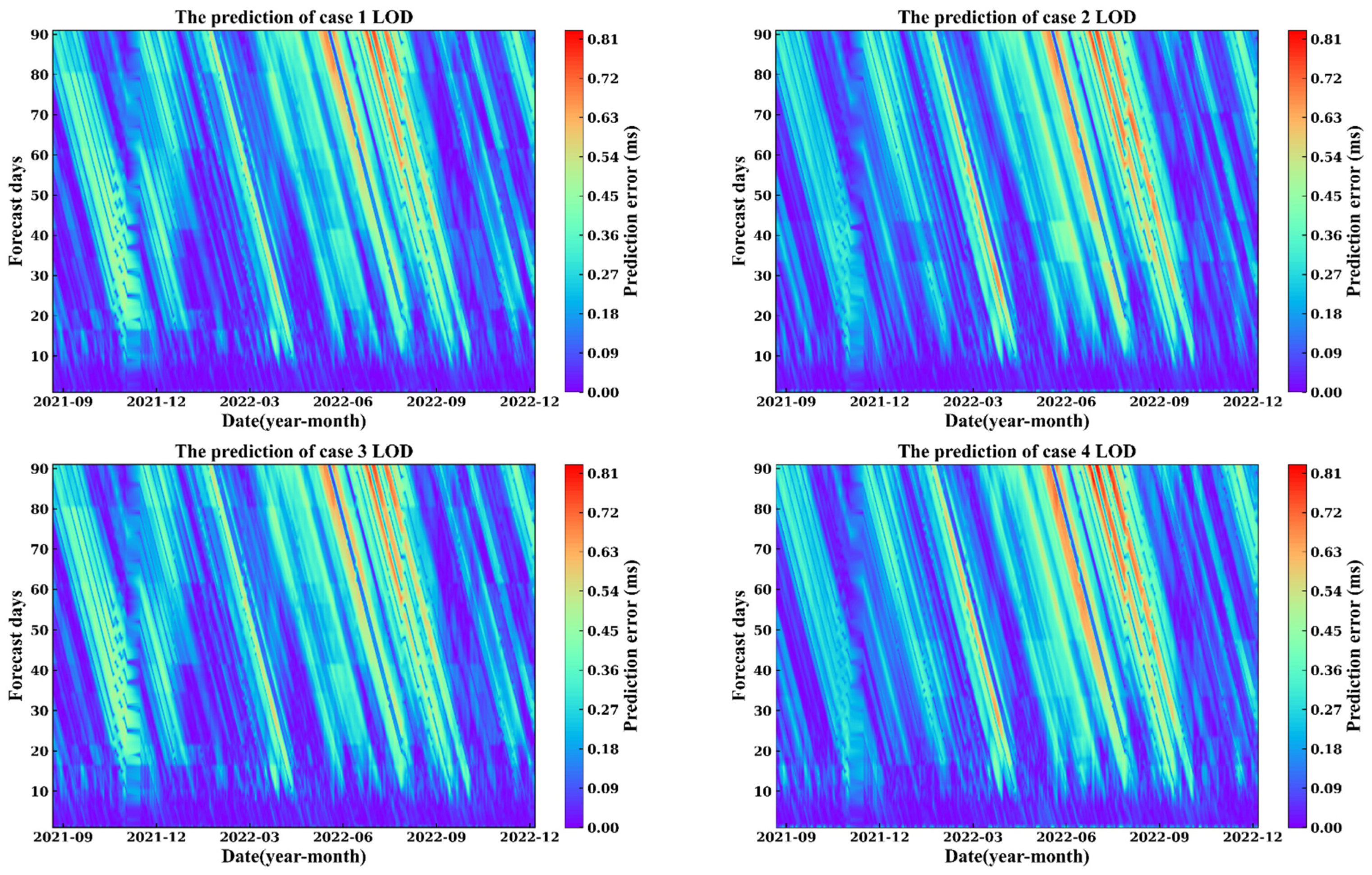
In the time span from September 2021 to December 2022, more than 430 UT1-UTC forecast experiments were conducted. The calculated results were compared with the UT1-UTC data provided by EOP C04, as shown in Figure 7.

In Figure 7, Case 1 represents the final solution in this paper. It utilizes a method based on denoising the EAM dataset + LS + AR. The construction of the denoising EAM dataset is described in detail in Section 2.2, including using GAM to denoise the observed dataset of EAM and using Kalman filtering to denoise the 6-day forecast data of EAM. In the least-squares fitting, periodic components of 23.9 days and 91.3 days are added; Case 2 also uses the denoising EAM dataset + LS + AR method. The difference from Case 1 is that it does not include the 23.9 days and 91.3 days periodic components; Case 3 adopts the method based on denoising the observed EAM dataset + LS + AR. The difference from Case 1 is that it does not apply Kalman filtering to denoise the 6-day forecast data of EAM; Case 4 is the prediction of ID 101 in the second EOPPCC method, which is presented in [39]. It is based on EAM + LS + AR and does not involve denoising the EAM dataset or adding the 23.9 days and 91.3 days periodic components; Bulletin A refers to the forecast results from IERS/USNO, which are used for comparison and validation.

From Figure 7, it can be seen that in the 1–6 days forecast, Case 1 performs significantly better than Case 3, Case 4, and Bulletin A. In the forecast of 7–80 days, Case 1 outperforms Case 2, Case 4, and Bulletin A. As for Case 3, its MAE almost overlaps with Case 1 after a 10 days forecast period. However, there is a notable improvement in MAE within the 1–10 days forecast span, indicating the necessity of applying Kalman filtering to denoise the EAM dataset and indirectly demonstrating the presence of noise in the EAM dataset. The main differences between Case 1 and Case 2 happen after 27 days, where Case 1 performs significantly better than Case 2 in the 27–90 days forecast, especially from 30 to 60 days. From the forecast results, it is demonstrated that including the 23.9 days and 91.3 days periodic components in the LS fitting can improve the 27–90 days prediction.

The 23.9 days and 91.3 days tidal terms marginally identified in the Fourier spectra of the EAM and GAM dataset belong to the Mm and Sta tidal components, with amplitudes about 10 and 6 us, respectively [46,48]. Currently, the IERS tidal model includes 62 harmonic tidal terms with periods from 5 days to 18.6 years [46], Ray and Erofeeva [48] propose an 80-term LOD tidal model, which is supposed to have better performance for the Sa, Ssa, Mf, and Mt tidal components. It is noted that all these main tidal components have been included in our LS fittings of GAM and EAM data.

Table 1. MAE for different prediction intervals for UT1-UTC (ms). Reduction A represents the improvement in prediction accuracy of Case 1 relative to Bulletin A, the Reduction 4 represents the improvement in prediction accuracy of Case 1 relative to Case 4.

MAE	Case 1	Case 2	Case 3	Case 4	Bulletin A	Reduction A	Reduction 4
0 days	0.0492	0.0492	0.0492	0.0492	0.0477	−3.14%	0
1 day	0.0557	0.0555	0.0582	0.0625	0.0638	12.70%	10.88%
2 days	0.0697	0.0697	0.0760	0.0868	0.0925	24.65%	19.70%
3 days	0.0876	0.0878	0.0975	0.1147	0.1268	30.91%	23.63%
4 days	0.1084	0.1095	0.1224	0.1461	0.1614	32.84%	25.80%
5 days	0.1328	0.1337	0.1513	0.1806	0.1956	32.11%	26.47%
6 days	0.1592	0.1604	0.1812	0.2175	0.2319	31.35%	26.80%
10 days	0.3603	0.3674	0.3836	0.4482	0.4317	16.54%	19.61%
15 days	0.8637	0.8766	0.8832	1.0258	0.9179	5.90%	15.80%
20 days	1.4804	1.4998	1.4930	1.6782	1.6257	8.94%	11.79%
25 days	2.1872	2.2153	2.1928	2.3836	2.4756	11.65%	8.24%
30 days	2.9169	3.0532	2.9081	3.1859	3.3373	12.60%	8.44%
35 days	3.5196	3.8481	3.5072	3.9641	4.0882	13.91%	11.21%
40 days	4.1864	4.6201	4.1675	4.7416	4.7224	11.35%	11.71%
45 days	4.8472	5.3831	4.8271	5.5233	5.3547	9.48%	12.24%
50 days	5.6589	5.9098	5.6644	6.0611	5.9999	5.68%	6.64%
55 days	6.2291	6.4405	6.2257	6.5919	6.8544	9.12%	5.50%
60 days	6.7857	6.9512	6.7813	7.2770	7.7938	12.93%	6.75%
65 days	7.5204	7.6214	7.5117	7.9717	8.6121	12.68%	5.67%
70 days	8.2271	8.3017	8.2528	8.5370	9.2820	11.37%	3.63%
75 days	8.8524	9.0037	8.8627	9.0730	9.7400	9.11%	2.43%
80 days	9.4235	9.6502	9.4215	9.6683	9.8954	4.77%	2.53%
85 days	10.1537	10.4142	10.1360	10.3865	10.0865	−0.67%	2.24%
90 days	10.9139	11.1243	10.8754	11.1187	10.3257	−5.70%	1.84%

presents the MAE of more than 430 forecast experiments with time spans from September 2021 to December 2022. In order to strictly compare the forecast accuracy with Bulletin A, the same forecast history data as Bulletin A was chosen in this study. Specifically, the forecast history data used was a combination of the final product of IERS C04 and the Bulletin A data from the most recent month. Among the more than 430 predictions, the case scenario on day 0 had a slight difference of 1.5 us compared to the UT1-UTC dataset of day 0 in Bulletin A. This difference was mainly due to missing files in several days of case data during the forecast period from September 2021 to December 2022.

From Table 1, it can be observed that in the 430 forecast experiments from September 2021 to December 2022, Case 1 outperformed Case 4 in the 1–90 days forecast span. This improvement is particularly significant in the short-term forecasts of 1–6 days. This can be attributed to the importance of the EAM dataset in the 1–6 days predictions of UT1-UTC and LOD. The improvements decreased at longer forecast days. Specifically, on the 6 days, 10 days, 30 days, 60 days, and 90 days, the MAE decreased by 26.80%, 19.61%, 8.44%, 6.75%, and 1.84%, respectively. Furthermore, Case 1 outperformed Bulletin A in the forecast spans of 1–80 days and exhibited a particularly significant improvement in the accuracy of 1–6 days forecasts. In the forecast spans of 6 days, 10 days, 30 days, and 60 days, the MAE decreased by 31.35%, 16.54%, 12.60%, and 12.93%, respectively. It is worth mentioning that in the forecast span of 80–90 days, Bulletin A exhibited a significant slowdown in the growth rate of MAE, demonstrating excellent performance.

3.3. Comparison of LOD Forecasts with IERS

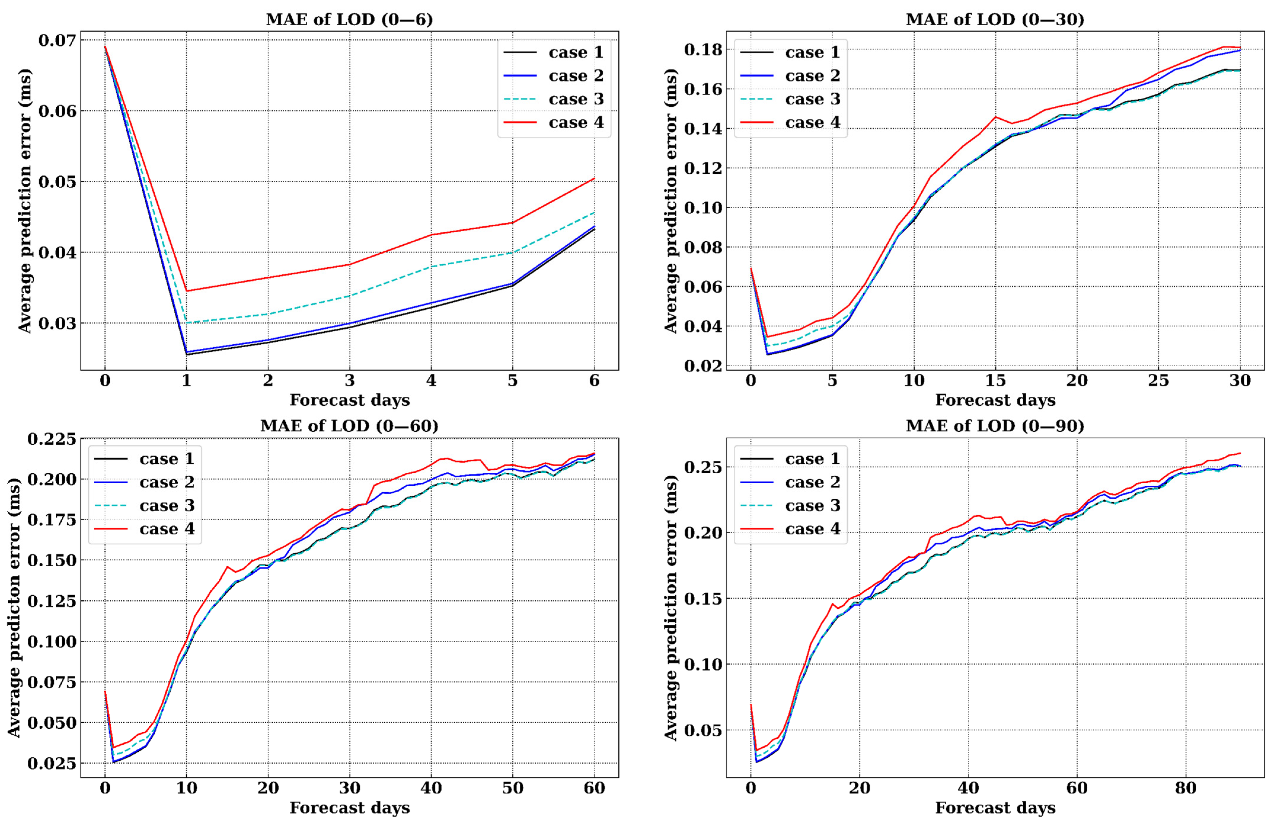
In the time span from September 2021 to December 2022, more than 430 LOD forecast experiments were conducted. The calculated results were compared with the LOD data provided by EOP C04, as shown in Figure 8.

In Figure 8, the solutions for Case 1, Case 2, Case 3, and Case 4 can be referenced in Section 3.2. They are consistent with the description in Section 3.2, with the only difference being that the LOD data have been forecasted. Due to the absence of forecast data for LOD in Bulletin A, only the forecast accuracy of these four case scenarios was compared from 1 to 90 days. The reason for the larger historical LOD data on day 0 is that the LOD data in Bulletin A is lagging, so we differentiate the UT1-UTC data from Bulletin A to obtain the 0-day’s LOD.

From Figure 8 and

Table 2. MAE for different prediction intervals for LOD (ms). The Reduction 4 represents the improvement in prediction accuracy of Case 1 relative to Case 4, the Reduction 3 represents the improvement in prediction accuracy of Case 1 relative to Case 3, the Reduction 2 represents the improvement in prediction accuracy of Case 1 relative to Case 2.

MAE	Case 1	Case 2	Case 3	Case 4	Reduction 4	Reduction 3	Reduction 2
0 days	0.0690	0.0690	0.0690	0.0690	0	0	0
1 day	0.0255	0.0259	0.0300	0.0345	26.09%	15.00%	1.54%
2 days	0.0272	0.0276	0.0312	0.0364	25.27%	12.82%	1.45%
3 days	0.0293	0.0299	0.0338	0.0382	23.30%	13.31%	2.01%
4 days	0.0321	0.0328	0.0379	0.0424	24.29%	15.30%	2.13%
5 days	0.0352	0.0355	0.0399	0.0441	20.18%	11.78%	0.85%
6 days	0.0432	0.0436	0.0456	0.0504	14.29%	5.26%	0.92%
10 days	0.0935	0.0944	0.0947	0.1006	7.06%	1.28%	0.95%
15 days	0.1308	0.1317	0.1320	0.1457	10.23%	0.91%	0.68%
20 days	0.1465	0.1451	0.1464	0.1527	4.06%	−0.06%	−0.96%
25 days	0.1572	0.1647	0.1564	0.1681	6.48%	−0.51%	4.55%
30 days	0.1694	0.1794	0.1690	0.1809	6.36%	−0.23%	5.57%
35 days	0.1828	0.1913	0.1824	0.1991	8.19%	−0.22%	4.44%
40 days	0.1953	0.1996	0.1949	0.2088	6.47%	−0.21%	2.15%
45 days	0.1995	0.2025	0.1992	0.2115	5.67%	−0.15%	1.48%
50 days	0.2028	0.2061	0.2028	0.2086	2.78%	0%	1.60%
55 days	0.2018	0.2051	0.2016	0.2085	3.21%	−0.10%	1.61%
60 days	0.2121	0.2151	0.2119	0.2159	1.76%	−0.09%	1.39%
65 days	0.2242	0.2289	0.2243	0.2313	3.07%	0.04%	2.05%
70 days	0.2264	0.2307	0.2261	0.2341	3.29%	−0.13%	1.86%
75 days	0.2337	0.2350	0.2334	0.2387	2.09%	−0.13%	0.55%
80 days	0.2446	0.2448	0.2442	0.2495	1.96%	−0.16%	0.08%
85 days	0.2480	0.2481	0.2474	0.2548	2.67%	−0.24%	0.04%
90 days	0.2505	0.2507	0.2504	0.2603	3.76%	−0.04%	0.08%

, it can be seen that Case 1 shows a particularly significant improvement in short-term forecasts (1–6 days) compared to Case 4, with an increase of over 14%. On the forecast span of 7–90 days, Case 1 performs better than Case 2. Specifically, on the 1st, 6th, 10th, 30th, 60th, and 90th days, Case 1 improves by 26.09%, 14.29%, 7.06%, 6.36%, 1.76%, and 3.76%, respectively, compared to Case 4. In comparison to Case 2, Case 1 shows more significant improvements in the forecast span of 25–75 days. Compared to Case 3, Case 1 exhibits particularly significant improvements in the forecast span of 1–6 days. These findings are consistent with the performance of UT1-UTC.

4. Discussion

4.1. Discussion on Order of AR Model

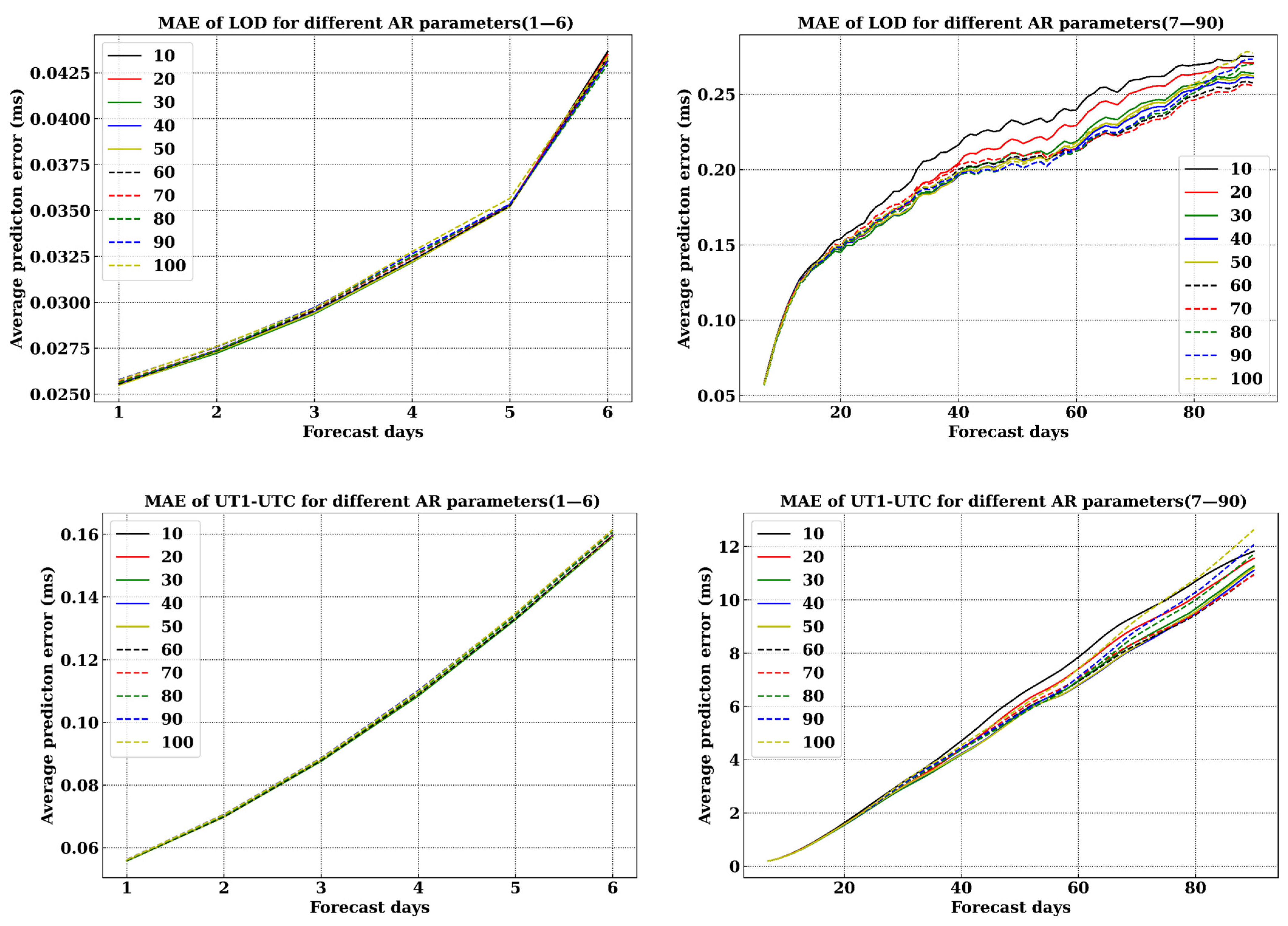
From September 2021 to December 2022, more than 430 short-term forecasts (1–6 days) and medium to long-term forecasts (7–90 days) of UT1-UTC and LOD were compared using different orders of AR models in terms of MAE. For the 1–6 days forecast, the AR model order within the range of 10 to 100 was searched when dealing with the fitting residual of GAM-EAM. For the 7–90 days forecast, the AR model order within the range of 10 to 100 was searched when dealing with the fitting residual of Full GAM.

From Figure 9, it can be seen that for short-term forecasts of 1–6 days, the choice of AR order is not critical. For UT1-UTC, different AR orders result in a difference of 2 us in MAE on the sixth day, while for LOD, the difference is only 0.7 us. However, for forecasts of 7–90 days, the impact of different AR orders is more significant. For UT1-UTC, different AR orders result in a difference of 1.705 ms in MAE on the 90th day, while for LOD, the difference is 0.022 ms.

4.2. Discussion on Prediction Error

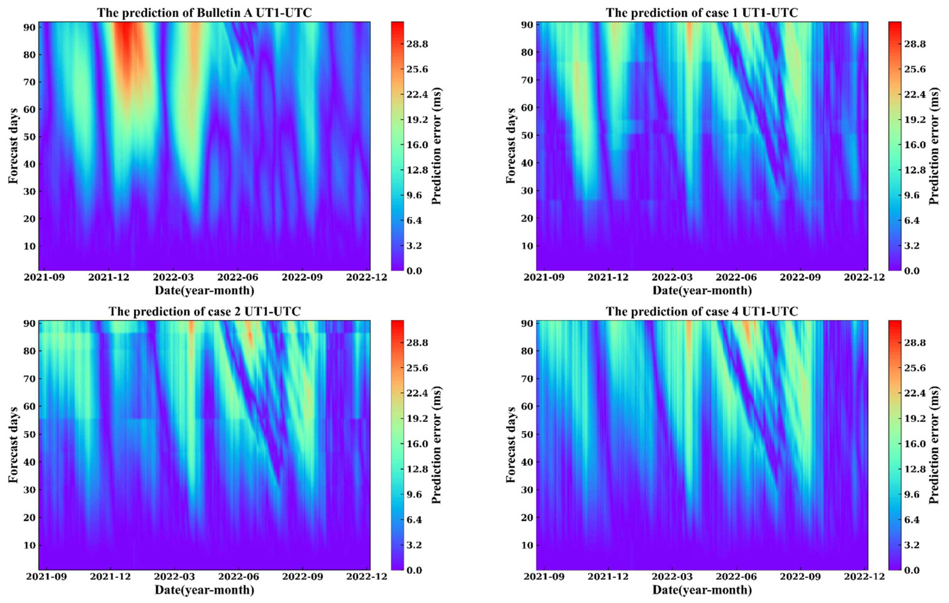
To analyze the forecasting accuracy in detail, a graph will be plotted for more than 430 forecasts of UT1-UTC and LOD errors from September 2021 to December 2022, ranging from 1 to 90 days.

As shown in Figure 10, UT1-UTC has a forecast error within 30 ms for a forecast span of 1–90 days. In the vicinity of December 2021, Bulletin A exhibited a significant forecast error for a forecast span of 30–90 days, which was not observed in the case scenario. Case 1 showed significant improvement in the forecast span of 30–80 days during September to November 2021 and December 2021 to March 2022.

Figure 11 displays that LOD has a forecast error within 0.9 ms for a forecast span of 1–90 days. Compared to Case 2 and Case 4, Case 1 exhibited significant improvement during December 2021 to June 2022. Case 1 and Case 3 performed almost identically in the medium to long-term forecast, mainly because Case 1 only underwent Kalman denoising of 1–6 days EAM forecast data relative to Case 3. Additionally, both UT1-UTC and LOD show a correlation between forecast performance and forecast time span. This is an interesting phenomenon, and based on Figure 10 and Figure 11, we can see that the prediction accuracy deteriorates in both semi-annual and annual cycles over the 1–90 day forecast span for both UT1 and LOD during September 2021 to December 2022. Specifically, all four scenarios showed a deterioration in forecast accuracy in September 2021, March 2022, and September 2022.

This phenomenon has been discussed in previous studies, suggesting that it may be caused by deteriorating observation quality or geophysical signals. For example, Dill et al. [36] mentioned that EAM can detect short-term and high-frequency deviations of long-term periodic signals in recent geophysical excitations, which have a sustained positive impact on EOP predictions for the next 90 days. Wu et al. [50] pointed out that the decrease in global flights due to the COVID-19 pandemic may deteriorate the quality of meteorological radar data, which may result in deteriorated weather and AAM forecasting. Xu et al. [51] mentioned that the occurrence of the La Nina phenomenon can cause anomalies of LOD and EAM.

From Figure 2 in this paper, it can be observed that GAM and EAM exhibit strong semi-annual and annual periodic components. The strong periodic variations in the Earth’s rotation may also be reflected in EOP predictions. Even though the semi-annual and annual periodic components are considered during least-squares modeling, it may not completely avoid the influence of strong periodic components in the forecasts. Some phenomena in the forecast data may also be related to certain geophysical processes, which deserves further investigation.

4.3. Perspective on UT1-UTC and LOD Forecast

In this study, for Case 1, the UT1/LOD forecast on the 10th day had an MAE of 0.3603 ms and 0.0935 ms, respectively. According to the statistical data collected by Tomasz et al. [38] based on the second EOP PCC during the period from 1 September 2021 to 29 May 2022, the MAE of UT1/LOD on the 10th day ranged from 0.36 to 3.13 ms and 0.07 to 0.28 ms. It is worth noting that there are some differences between the evaluation methods used in this article and the second EOP PCC. This article evaluates on a daily basis, while the second EOP PCC evaluates on a weekly basis. Additionally, this article uses approximately 400 files for MAE evaluation, while the second EOP PCC only uses around 60 files. Using a fixed interval of one file per week can to some extent reflect the forecast accuracy but may also introduce some randomness. Therefore, due to the different number of files used and the evaluation time units, there may be differences in the evaluation results between this article and the second EOP PCC evaluation. The Case 1 scheme in this study is an improvement on the forecasting method proposed in Dill [36], which first proposes denoising of the EAM dataset based on the use of EAM + LS + AR, and conducts research on forecast using the denoised EAM dataset. In addition, parameter optimization was performed, including the determination of the AR order and the selection of the least-squares periodic terms.

The algorithm used in this paper, based on denoising EAM + LS + AR, is more complex and accurate compared to the traditional LS + AR algorithm. This algorithm requires daily updates of the EAM dataset, and if there is an interruption in the EAM dataset, the daily forecasts cannot be completed. Fortunately, apart from GFZ, Eidgenössische Technische Hochschule (ETH) Zurich also provides EAM predictions [52,53,54]. However, there is still a lack of accuracy estimation in the EAM data, and our research also indicates the feasibility for improvement in EAM. Due to the significance of EAM data, the evaluation and improvement in EAM accuracy will be one of the key issues in future EOP forecasting.

For further research on EOP forecasting, the 14-day EAM predictions provided by ETH Zurich can be utilized. It is important to note that the method described in this paper is highly sensitive to the accuracy of the dataset, especially the initial values on day 0. Additionally, the choice of AR order is closely related to the data and may require periodic adjustments to achieve optimal forecasting. In future research, the combination of machine learning algorithms, such as incorporating long short-term memory (LSTM), can be employed to further improve the accuracy of EOP predictions.

Based on the comparison of UT1-UTC and LOD forecasts, the following points of view are proposed:

(a)

According to the comparison between Case 1 and Case 2, as well as the GAM spectrum analysis results, we plan to evaluate and use an improved tidal model for EOP forecasting research in the future, for example, Ray and Erofeeva [48], to expand the 62 solid Earth tidal constituents in future IERS Conventions’ tidal models.

(b)

Comparing Case 1 with Bulletin A, it is evident that the EAM forecast dataset has a significant impact on short-term UT1-UTC and LOD forecasts. Therefore, it is recommended to consider using geophysical models or ML techniques to extend the 6-day EAM forecast to 10–15 days and then conduct corresponding UT1/LOD forecast experiments.

(c)

The forecasts are sensitive to initial conditions. It is suggested that combination algorithms to improve the accuracy of the initial values of UT1-UTC and LOD on day 0 are used.

(d)

This study used a preliminary denoising method on the EAM and EAM 1–6 days forecast datasets, but a detailed investigation has not been conducted. Future research could focus on specific accuracy studies for the EAM dataset and its forecast dataset to provide estimations on the uncertainties of the EAM dataset.

5. Conclusions

This study adopted the UT1-UTC and LOD forecasting algorithm of EAM+LS+AR. The GAM dataset was used to denoise the EAM observation dataset, and the Kalman filter was used to denoise the 6-day forecast dataset of EAM. Through spectrum analysis of GAM and EAM, periodic terms of 23.9 days and 91.3 days were marginally identified, and comparison experiments on these two terms were conducted. In a total of over 430 UT1-UTC and LOD forecasting experiments for the period from September 2021 to December 2022, with forecast horizons ranging from 1 to 90 days, the following main conclusions were drawn:

(a)

Through the UT1-UTC and LOD forecast comparison experiments of Case 1, Case 3, and Case 4, it has been demonstrated that using GAM and Kalman filtering to denoise the EAM and EAM 6-day forecast data can significantly improve the forecast accuracy of UT1-UTC and LOD. The improvement is particularly significant in the short-term forecast of 1–6 days, which also confirms the effectiveness of noise suppression of EAM on EOP predictions.

(b)

By comparing the UT1-UTC and LOD between Case 1 and Case 2, we found that adding the least-squares fitting periodic terms of 23.9 days and 91.3 days can significantly improve the forecast accuracy in the medium-to-long term of 30–80 days. This means model fitting of tidal components with an amplitude of 5 us can enhance the accuracy of the forecast.

(c)

Through the GAM spectral analysis, it is confirmed that the Earth tidal models from the IERS 2010 Conventions proposed in the 1980s and 1990s cannot fully compensate for tidal effects. This suggests that we need to continuously improve and adopt better tidal models in studies of geodynamics, Earth rotation, and EOP measurement and predictions.

Using the GAM dataset and Kalman filtering algorithm to denoise EAM and EAM 6-day forecast data can effectively improve the forecast accuracy of UT1-UTC and LOD, especially in short-term forecasts. In addition, the choice of the least-squares fitting periodic term significantly affects the forecast accuracy of UT1-UTC and LOD. Furthermore, the historical dataset based on the forecasting algorithm is crucial for the accuracy of the forecast.

References

1. Nastula, J.; Chin, T.M.; Gross, R.; Sliwinska, J.; Winska, M. Smoothing and predicting celestial pole offsets using a Kalman filter and smoother. J. Geod. 2020, 94, 2–17. [Google Scholar] [CrossRef]
2. Gambis, D.; Luzum, B. Earth rotation monitoring, UT1-UTC determination and prediction. Metrologia 2011, 48, 165–170. [Google Scholar] [CrossRef]
3. Gambis, D. Monitoring earth orientation using space-geodetic techniques: State of the art and prospective. J. Geod. 2004, 78, 295–303. [Google Scholar] [CrossRef]
4. Kalarus, M.; Schuh, H.; Kosek, W.; Akyilmaz, O.; Bizouard, C.; Gambis, D.; Gross, R.; Jovanovi’c, B.; Kumakshev, S.; Kutterer, H.; et al. Achievements of the Earth orientation parameters prediction comparison campaign. J. Geod. 2010, 84, 587–596. [Google Scholar] [CrossRef]
5. Schuh, H.; Ulrich, M.; Egger, D.; Müller, J.; Schwegmann, W. Prediction of Earth orientation parameters by artificial neural networks. J. Geod. 2002, 76, 247–258. [Google Scholar] [CrossRef]
6. Schuh, H.; Johannes, B.; Heinkelmann, R.; Hobiger, T.; Jorge, M.C.P.; Pany, A.; Tanir, E.; Teke, K.; Todorova, S. International VLBI Service for Geodesy and Astrometry 2006 Annual Report. No. NASA/TP-2007-214151. 2007; pp. 208–211. Available online: https://ivscc.gsfc.nasa.gov/publications/ar2006/IVS-2006-Annual-Report.pdf (accessed on 12 August 2023).
7. Nilsson, T.; Böhm, J.; Schuh, H. Sub-diurnal earth rotation variations observed by VLBI. Artif. Satell. 2010, 45, 49–55. [Google Scholar] [CrossRef]
8. Nilsson, T.; Böhm, J.; Schuh, H. Universal time from VLBI single-baseline observations during CONT08. J. Geod. 2011, 85, 415–423. [Google Scholar] [CrossRef]
9. Nilsson, T.; Heinkelmann, R.; Karbon, M.; Raposo-Pulido, V.; Soja, P.; Schuh, H. Earth orientation parameters estimated from VLBI during the CONT11 campaign. J. Geod. 2014, 88, 491–502. [Google Scholar] [CrossRef]
10. Byram, S.; Hackman, C. High-precision GNSS orbit, clock and EOP estimation at the United States Naval Observatory. In Proceedings of the 2012 IEEE/ION Position, Location and Navigation Symposium, Myrtle Beach, SC, USA, 23–26 April 2012. [Google Scholar] [CrossRef]
11. Mireault, Y.; Kouba, J. IGS earth rotation parameters. GPS Solut. 1999, 3, 59–72. [Google Scholar] [CrossRef]
12. Zajdel, R.; Sośnica, K.; Bury, G.; Dach, R.; Prange, L. System-specific systematic errors in earth rotation parameters derived from GPS, GLONASS, and Galileo. GPS Solut. 2020, 24, 74. [Google Scholar] [CrossRef]
13. Hein, G.W. Status, perspectives and trends of satellite navigation. Satell. Navig. 2020, 1, 22. [Google Scholar] [CrossRef] [PubMed]
14. Coulot, D.; Pollet, A.; Collilieux, X.; Berio, P. Global optimization of core station networks for space geodesy: Application to the referencing of the SLR EOP with respect to ITRF. J. Geod. 2010, 84, 31. [Google Scholar] [CrossRef]
15. Pavlov, D. Role of lunar laser ranging in realization of terrestrial, lunar, and ephemeris reference frames. J. Geod. 2020, 94, 5. [Google Scholar] [CrossRef]
16. Pearlman, M.R.; Degnan, J.J.; Bosworth, J.M. The international laser ranging service. Adv. Space Res. 2002, 30, 135–143. [Google Scholar] [CrossRef]
17. Angermann, D.; Seitz, M.; Drewes, H. Analysis of the DORIS contributions to ITRF2008. Adv. Space Res. 2010, 46, 1633–1647. [Google Scholar] [CrossRef]
18. Moreaux, G.; Lemoine, F.G.; Capdeville, H.; Kuzin, S.; Otten, M.; Stepanek, P.; Willis, P.; Ferrage, P. The international DORIS service contribution to the 2014 realization of the international terrestrial reference frame. Adv. Space Res. 2016, 58, 2479–2504. [Google Scholar] [CrossRef]
19. Willis, P.; Fagard, H.; Ferrage, P.; Lemoine, F.G.; Noll, C.E.; Noomen, R.; Otten, M.; Ries, J.C.; Rothacher, M.; Soudarin, L.; et al. The international DORIS service (IDS): Toward maturity. Adv. Space Res. 2010, 45, 1408–1420. [Google Scholar] [CrossRef]
20. Ratcliff, J.T.; Gross, R.S. Combinations of Earth orientation measurements: SPACE2008, COMB2008, and POLE2008. JPL Publ. 2010, 10–14, 1–27. [Google Scholar]
21. Artz, T.; Bernhard, L.; Nothnagel, A.; Steigenberger, P.; Tesmer, S. Methodology for the combination of sub-daliy earth rotation from GPS and VLBI observations. J. Geod. 2012, 86, 221–239. [Google Scholar] [CrossRef]
22. Bizouard, C.; Lambert, S.; Gattano, C.; Becker, O.; Richard, J.-Y. The IERS EOP 14C04 solution for Earth orientation parameters consistent with ITRF 2014. J. Geod. 2019, 93, 621–633. [Google Scholar] [CrossRef]
23. Gambis, D.; Bizouard, C. Monitoring UT1-UTC from astrogeodetic techniques at the EOP Center of the IERS. In Proceedings of the 28th IAU General Assembly, Beijing, China, 20–31 August 2012; International Astronomical Union: Paris, France, 2009; pp. 207–208. [Google Scholar]
24. Akulenko, L.D.; Kumakshev, S.A.; Markov, Y.G. Motion of the Earth’s pole. Dokl. Phys. 2002, 47, 78–84. [Google Scholar] [CrossRef]
25. Akulenko, L.D.; Kumakshev, S.A.; Rykhlova, L.V. A model for the polar motion of the deformable Earth adequate for astrometric data. Astron. Rep. 2002, 46, 74–82. [Google Scholar] [CrossRef]
26. Akulenko, L.D.; Kumakshev, S.A.; Rykhlova, L.V. Forecasting the polar motions of the deformable Earth. Astron. Rep. 2002, 46, 858–866. [Google Scholar] [CrossRef]
27. Kosek, W.; Kalarus, M.; Niedzielski, T. Forecasting of the Earth orientation parameters comparison of different algorithms. In The Celestial Reference Frame for the Future, Proceedings of the Journèes 2007 Systèmes Deréférence Spatio-Temporels, Paris, France, 17–19 September 2007; Capitaine, N., Ed.; Observatoire de Paris, Systèmes de RéférenceTemps-Espace: Paris, France, 2008; pp. 155–158. [Google Scholar]
28. Guo, J.Y.; Li, Y.B.; Dai, C.L.; Shum, C.K. A technique to improve the accuracy of Earth orientation prediction algorithms based on least squares extrapolation. J. Geodyn. 2013, 70, 36–48. [Google Scholar] [CrossRef]
29. Wang, Q.J.; Liao, D.C.; Zhou, Y.H. Real-time rapid prediction of variations of Earth’s rotational rate. Chin. Sci. Bull. 2008, 53, 969–973. [Google Scholar] [CrossRef]
30. Yu, L.; Guo, M.; Hu, D.D.; Cai, H.-B.; Zhao, D.-N.; Hu, Z.-P.; Gao, Y.-P. Short-term prediction of UT1-UTC-UTC by combination of the grey model and neural networks. Adv. Space Res. 2017, 59, 524–531. [Google Scholar]
31. Kosek, W.; Kalarus, M.; Johnson, T.J.; Wooden, W.H.; McCarthy, D.D.; Popinski, W. A comparison of LOD and UT1-UTC-UTC forecasts by different combination prediction techniques. Artif. Satell. 2005, 40, 119–125. Available online: https://www.researchgate.net/publication/236149838 (accessed on 13 August 2023).
32. Kosek, W.; Kalarus, M.; Johnson, T.J.; Wooden, W.H.; McCarthy, D.D.; Popinski, W. A comparison of UT1-UTC-UTC forecasts by different prediction techniques. Proc. Journeys Syst. De Ref. Spatiotemporal 2004, 140–141. Available online: https://www.researchgate.net/publication/263529654 (accessed on 13 August 2023).
33. Freedman, A.P.; Steppe, J.A.; Dickey, J.O.; Eubanks, T.M.; Sung, L.Y. The short-term prediction of universal time and length of day using atmospheric angular momentum. J. Geophys. Res. 1994, 99, 6981–6996. [Google Scholar] [CrossRef]
34. Gross, R.S.; Eubanks, T.M.; Steppe, J.A.; Freedman Dickey, J.O.; Runge, T.F. A Kalman filter-based approach to combining independent Earth-orientation series. J. Geod. 1998, 72, 215–235. [Google Scholar] [CrossRef]
35. Xu, X.Q.; Zhou, Y.H.; Liao, X.H. Short-term earth orientation parameters predictions by combination of the least-squares, AR model and Kalman filter. J. Geodyn. 2012, 62, 83–86. [Google Scholar] [CrossRef]
36. Dill, R.; Dobslaw, H.; Thomas, M. Improved 90-day Earth orientation predictions from angular momentum forecasts of atmosphere, ocean, and terrestrial hydrosphere. J. Geod. 2019, 93, 287–295. [Google Scholar] [CrossRef]
37. Yang, Y.G.; Xu, T.H.; Sun, Z.Z.; Nie, W.F.; Fang, Z.L. Middle- and Long-Term UT1-UTC-UTC Prediction Based on Constrained Polynomial Curve Fitting, Weighted Least Squares and Autoregressive Combination Model. Remote Sens. 2022, 14, 3252. [Google Scholar] [CrossRef]
38. Tomasz, K.; Henryk, D.; Justyna, Ś.; Jolanta, N.; Małgorzata, W.; Aleksander, P. Evaluation of selected short-term predictions of UT1-UTC-UTC and LOD collected in the second earth orientation parameters prediction comparison campaign. Earth Planets Space 2022, 74, 191. [Google Scholar] [CrossRef]
39. Yang, X.Y.; Wu, Y.W.; Zhao, X.; Yang, X.H.; Zhang, S.G. Piecewise UT1-UTC prediction based on the Earth’s fluid effective angular momentum function. J. Time Freq. 2023, 46, 94–104. [Google Scholar]
40. Jungclaus, J.H.; Fischer, N.; Haak, H.; Lohmann, K.; Marotzke, J.; Matei, D.; Mikolajewicz, U.; Notz, D.; VonStorch, J.S. Characteristics of the ocean simulations in the Max Planck Institute Ocean Model (MPIOM) the ocean component of the MPI-Earth system model. J. Adv. Model. Earth Syst. 2013, 5, 422–446. [Google Scholar] [CrossRef]
41. Dill, R. Hydrological Model LSDM for Operational Earth Rotation and Gravity Field Variations; Scientific Technical Report STR 08/09; GFZ: Potsdam, Germany, 2008; p. 35. [Google Scholar]
42. Dobslaw, H.; Dill, R. Predicting earth orientation changes from global forecasts of atmosphere hydrosphere dynamics. Adv. Space Res. 2018, 61, 1047–1054. [Google Scholar] [CrossRef]
43. Dobslaw, H.; Dill, R. Product Description Document: Effective Angular Momentum Functions from Earth System Modelling at GeoForschungsZen truminPotsdam. 2019. Available online: http://rz-vm115.gfz-potsdam.de:8080/repository/entry/show?entryid=e8e59d73-c0c2-4a9d-b53b-f2cd70f85e28 (accessed on 12 August 2023).
44. Tamisiea, M.E.; Hill, E.M.; Ponte, R.M.; Davis, J.L.; Velicogna, I.; Vinogradova, N.T. Impact of self-attraction and loading on the annual cycle in sea level. J. Geophys. Res. 2010, 115, 1–15. [Google Scholar] [CrossRef]
45. Hagemann, S.; Dumenil, L. A parametrization of the waterflow for the global scale. Clim. Dynam. 1998, 14, 17–31. [Google Scholar] [CrossRef]
46. Petti, G.; Luzum, B. IERS Conventions 2010; Verlag des Bundesamts für Kartographie und Geodäsie: Frankfurt am Main, Germany, 2010; ISBN 3-89888-989-6. [Google Scholar]
47. Barnes, R.T.H.; Hide, A.; White, A.; Wilson, C.A. Atmospheric angular momentum fluctuations. Length-of-day changes and polar motion. Proc. R. Soc. Lond. Ser. A Math. Phys. Eng. Sci. 1983, 387, 31–73. [Google Scholar] [CrossRef]
48. Ray, R.D.; Erofeeva, S.Y. Long-period tidal variations in the length of day. J. Geophys. Res. 2014, 119, 1498–1509. [Google Scholar] [CrossRef]
49. Box, G.E.P.; Jenkins, G.M. Time Series Analysis: Forecasting and Control; Holden Day: San Francisco, CA, USA, 1976. [Google Scholar]
50. Wu, Y.W.; Zhao, X.; Yang, X.Y. Improved Prediction of polar motions by piecewise parameterization. Artif. Satell. 2022, 57, 290–299. [Google Scholar] [CrossRef]
51. Xu, X.-Q.; Zhou, Y.-H.; Duan, P.-S.; Fang, M.; Kong, Z.-Y.; Xu, C.-C.; An, X.-R. Contributions of oceanic and continental AAM to interannual variation in Delta LOD with the detection of 2020–2021 La Nina event. J. Geod. 2022, 96, 43. [Google Scholar] [CrossRef]
52. Kiani Shahvandi, M.; Gou, J.; Schartner, M.; Soja, B. Data driven approaches for the prediction of Earth’s effective angular momentum functions. In Proceedings of the IGARSS 2022—2022 IEEE International Geoscience and Remote Sensing Symposium, Kuala Lumpur, Malaysia, 17–22 July 2022; pp. 6550–6553. [Google Scholar]
53. Kiani Shahvandi, M.; Soja, B. Small geodetic datasets and deep networks: Attention-based residual LSTM autoencoder stacking for geodetic time series. In Machine Learning, Optimization, and Data Science, Proceedings of the 7th International Conference, LOD 2021, Grasmere, UK, 4–8 October 2021, Revised Selected Papers, Part I; Lecture Notes in Computer Science; Springer: Cham, Switzerland, 2021; Volume 13163. [Google Scholar] [CrossRef]
54. Soja, B.; Kiani Shahvandi, M.; Schartner, M.; Gou, J.; Kłopotek, G.; Crocetti, L.; Awadaljeed, M. The New Geodetic Prediction Center at ETH Zurich. In Proceedings of the New Geodetic Prediction Center at ETH Zurich, EGU General Assembly 2022, Vienna, Austria, 23–27 May 2022; p. EGU22-9285. [Google Scholar] [CrossRef]
Figure 1. GAM and EAM series from 2000 to 2023. The left graph shows the GAM series (shown as a blue dashed line), derived from the IERS C04 LODR sequence using Liouville’s equation. The green dashed line represents the EAM dataset, which is composed of AAM, OAM, HAM, and SLAM. The red line on the right side shows the difference between GAM and EAM. Both GAM and EAM are dimensionless.
Remotesensing 15 04654 g001
Figure 2. Fourier spectrum of geodetic excitation GAM (blue) modeled angular momentum function EAM (green), and the GAM-EAM (red); the right panel shows the sub-monthly Fourier spectrum.
Remotesensing 15 04654 g002
Figure 3. The blue dashed line in the left plot represents the GAM dataset from 2017 to 2022. The green solid line represents the GAM LS fitting curve, and the red line represents the GAM LS fitting residual. In the right plot, the blue dashed line represents the EAM dataset from 2017 to 2022. The green solid line represents the EAM LS fitting curve, and the red line represents the EAM LS fitting residual. The LS fitting residuals of GAM and EAM have been downward shifted by 1.4 × 10⁻⁸.
Remotesensing 15 04654 g003
Figure 4. The left plot shows the comparison between New EAM and EAM, while the right plot represents the difference between New EAM and EAM with respect to GAM.
Remotesensing 15 04654 g004
Figure 5. The black lines show the differences between the least-squares fitting residual of the EAM and the GAM, and the red lines show the differences between the least-squares fitting residual of the filtered EAM and GAM.
Remotesensing 15 04654 g005
Figure 6. Flowchart of EAM Denoising Process.
Remotesensing 15 04654 g006
Figure 7. The comparison of UT1-UTC forecast accuracy for the period of 0 to 90 days.
Remotesensing 15 04654 g007
Figure 8. The comparison of LOD forecast accuracy for the period of 0 to 90 days.
Remotesensing 15 04654 g008
Figure 9. The MAE of the UT1-UTC and LOD prediction values corresponding to different AR models.
Remotesensing 15 04654 g009
Figure 10. The absolute prediction error from 1 to 90 days in 430 UT1-UTC prediction experiments between 2021.09 and 2022.12.
Remotesensing 15 04654 g010
Figure 11. The absolute prediction error from 1 to 90 days in 430 LOD prediction experiments between 2021.09 and 2022.12.
Remotesensing 15 04654 g011