Imprint of Mesoscale Eddies on Air-Sea Interaction in the Tropical Atlantic Ocean

Abstract

This study investigates the effect of mesoscale eddies on air–sea heat and fresh water exchange in the tropical Atlantic Ocean (TAO) using 8 years of satellite altimetry data, combined with sea surface temperature (SST), latent and sensible heat fluxes (LHF and SHF), infrared fluxes (IRF) and precipitation (PR) data. Results indicate that approximately ∼40% of cyclonic eddies contribute to warm SST anomalies, and ∼40% of anticyclonic eddies contribute to cold SST anomalies. Eddies were found to play a role in the variability in LHF, SHF and IRF, contributing 10–35% of their total variability, with the largest contributions observed beneath the intertropical convergence zone (ITCZ) and frontal SST areas. Composite analysis of SST and heat flux anomalies over eddies suggested that the anomalies created through horizontal advection processes may not significantly impact the overall LHF, SHF and IRF over eddies, contrary to vertical processes. Despite a lack of clear correlation between heat flux and PR anomalies over eddies in the TAO, significant correlations were found beneath the ITCZ, suggesting that eddies may impact both heat fluxes and PR in the ITCZ region. This study provides an original contribution to the understanding of the impact of ocean mesoscale eddies on the atmosphere in the TAO.

1. Introduction

Over the past 30 years, extensive research has been conducted to describe and understand ocean mesoscale dynamics, made possible by the constellation of altimetry satellites that measure sea surface height. These measurements have revealed the widespread presence of energetic cyclonic and anticyclonic eddies (CE and AE, respectively), that have typical radii of several tens of kilometers and lifetimes lasting several months or years [1,2,3,4,5,6,7,8,9,10,11,12]. The vertical extent of mesoscale eddies can reach several hundred meters, impacting the ocean at depth [8,13,14,15,16,17,18,19]. These structures can trap water masses within their cores and transport them across long distances and they play a key role in the transport, mixing and redistribution of heat, salt, nutrients and other physical and biogeochemical tracers [20,21,22,23]. Recently, research has shown that oceanic eddies can significantly impact the atmosphere above them by altering ocean–atmosphere heat exchange, causing modification in wind characteristics, cloud coverage and precipitation (PR) [24,25]. In the Southern Ocean, for instance, heat transfer from the ocean to the atmosphere is increased above AEs, linked to positive sea surface temperature (SST) anomalies, leading to more convection, clouds and PR [25]. On the other hand, CEs with negative SST anomalies reduce heat exchange with the atmosphere and thus reduce convection, clouds and PR [25]. The impact of CEs and AEs on turbulent heat exchange at the ocean-atmosphere interface has also been studied in the South Atlantic, particularly in highly energetic eddy regions such as the Brazil–Malvinas confluence and the Agulhas Current retroflection [10]. Our study aims to fill the gap in the knowledge of the impact of mesoscale eddies on heat and freshwater exchange in the tropical Atlantic Ocean (TAO), a region of interest in this regard, in particular because of the possible impact on the African Monsoon.

The TAO is a vital component of the Earth’s climate system, playing a significant role in shaping the world’s weather patterns by exchanging heat, moisture and other important variables between the ocean and atmosphere [26]. Its location near the equator and high intensity of solar radiation result in higher sea surface temperatures (SST, Figure 1) and a positive heat balance, making it a key source of heat for the atmosphere [26]. This heat exchange leads to increased atmospheric turbulence and low-level wind speeds [24], driving deep atmospheric convection and the formation of the Intertropical Convergence Zone (ITCZ, Figure 1). The ITCZ, marked by cumulus and cumulonimbus clouds and heavy PR, represents an essential feature in the global water and energy cycles, affecting the distribution of PR, clouds, and atmospheric circulation across the tropics. The ITCZ’s seasonal migration from its northernmost position (approximately 8°N) in the boreal summer to its southernmost position (approximately 2°N) in the boreal winter (Figure 1) [27,28,29] also influences global wind patterns and ocean currents, making the TAO a critical component of the Earth’s climate system.

However, these complex processes in the TAO can also be influenced by mesoscale oceanic eddies that can have, as mentioned above, a significant impact on air–sea heat and moisture exchanges. Our study aims to investigate the imprint of these mesoscale eddies on air–sea interaction in the TAO, and in particular, in the ITCZ region, which is a key area for heat and moisture exchange between the ocean and atmosphere. In the Earth climate models (e.g., CPIM) small-scale structures are not taken into account explicitly, due to the coarse spatial resolution. Warm SST biases are mentioned in the CMIP estimations in the eastern part of the TAO [30] and might be due to the non representation of small-scale structures such as mesoscale eddies. A comprehensive understanding of the influence of mesoscale eddies on air–sea interaction in the TAO is thus crucial for improving our understanding and modeling of the Earth’s climate system.

In the TAO, mesoscale eddies have typical amplitudes of 1–5 cm and radii of 40–100 km, with the highest eddy kinetic energy (EKE) located in the western boundary in the North Brazil Current retroflection [1]. On average, TAO eddies persist for several months and can cross the Atlantic basin from east to west [1,7]. As shown by ARGO data, most of these eddies are located subsurface, with their maximum temperature and salinity anomalies located below the pycnocline [8,13]. A unique feature of these subsurface eddies is their inverse SST signature compared to surface intensified eddies, with negative SST anomalies for subsurface AEs and positive for CEs [13,14,31]. Referred to as “Inverse Eddy SST Anomalies” or “Abnormal Mesoscale Eddies”, they make up approximately one third of the global oceanic mesoscale eddy population [32]. The abnormal SST anomalies in mesoscale eddies have been linked to factors such as vertical mixing, particularly during ocean re-stratification in spring and early summer [13,33], or the surrounding large-scale SST distribution [13,34,35]. Indeed, the SST signature/anomaly of an eddy may change as it moves through different water masses and during its decay, through the absorption of surrounding water masses [35]. Thus, mesoscale eddies with inverse SST anomalies may impact ocean–atmosphere interactions differently from eddies with the same polarity but a normal SST signature, particularly at the seasonal scale. The aim of this study is to investigate the impact of these cold-core or warm-core eddies, regardless of their cyclonic or anticyclonic polarity, on latent heat fluxes (LHF), sensible heat fluxes (SHF), ocean infrared fluxes (IRF) at the ocean-atmosphere interface and their relationship with PR anomalies in the TAO region.

The paper first provides a detailed presentation of the dataset and methodology used. Then, it analyzes the SST anomalies across mesoscale eddies in the TAO to determine the presence of warm-core or cold-core eddies. This preliminary analysis serves as the foundation for the subsequent examination of the eddies’ influence on heat fluxes and PR anomalies.

2. Materials and Methods

The study period for all the data used extends from January 2010 to December 2017.

2.1. Altimetry Data and Mesoscale Eddy Tracking

In the present study, mesoscale eddies were detected and tracked from daily absolute dynamic topography (ADT) maps, which is a multimission satellite altimetry product, optimally interpolated onto a 0.25° × 0.25° longitude/latitude grid [36]. This product is freely distributed by the Copernicus Marine Environment Monitoring Service and available on https://marine.copernicus.eu/ (accessed on 15 February 2023).

The mesoscale eddies were detected using the eddy detection algorithm by [2,3], which defines the center of an eddy as a local maximum for AEs or a local minimum for CEs in the ADT maps, and the edge as the outermost closed ADT contours surrounding the center. After an eddy is detected, its properties such as amplitude, radius and EKE are derived. Eddy amplitude is defined as the absolute value of the ADT difference between the eddy center and the averaged ADT along the eddy edge. The radius of an eddy corresponds to the radius of an equivalent circular vortex having the same area, delimited by the eddy edge, while the EKE of an eddy is the average eddy kinetic energy over the considered eddy.

The eddy trajectories were reconstructed using the eddy tracking algorithm by [8]. To ensure robust results, we only considered eddies that lasted for a minimum of 30 days and had a median amplitude and radius greater than 1 cm and 30 km respectively, all along their trajectory. This approach is consistent with previous studies in TAO such as [1,13].

2.2. Sea Surface Temperature, Heat Fluxes and Precipitation Data

In order to investigate mesoscale eddy signatures on SST, we used the v2.1 version of the optimum interpolated sea surface temperature (OISST) analysis https://www.ncei.noaa.gov/products/ (accessed on 15 February 2023). The OISST product, formerly known as Reynolds SST, is a multi-platform product merging infrared satellite observations of the Advanced Very High-Resolution Radiometer and in situ measurements [37,38]. This dataset provides daily SST data on a grid with a resolution of 0.25° longitude by 0.25° latitude, with a good accuracy (bias = 0.04 °C and root mean square difference = 0.24 °C, see Table 3 in [37]).

To study the impact of mesoscale eddies on turbulent heat fluxes, we used the LHF and SHF products, version 4.1, provided by the Institut Français de Recherche pour l’Exploitation de la Mer (IFREMER, https://wwz.ifremer.fr/oceanheatflux/, accessed on 15 February 2023). These products offer daily global heat fluxes at a spatial-resolution of 0.25° × 0.25° in longitude and latitude. The computation of LHF and SHF is derived from atmospheric boundary layer parameters including wind-speed, air and SST and air specific humidity [39,40,41]. Ocean IRF is calculated based on the SST. The LHF, SHF and IRF are given by the following bulk formulae:

$$LHF=\rho C_E{L}_{v}U(q_s-q_a)$$

(1)

$$SHF=\rho C_p{C}_{h}U({\theta }_s-{\theta }_a)$$

(2)

$$IRF=ϵ\sigma {\left(SST\right)}^4$$

(3)

where ${\theta }_s$ and ${\theta }_a$ represent the sea surface and air (10 meters above sea level) temperature respectively, $q_s$ and $q_a$ denote the saturated and specific humidity in the air. The air density $\rho$ and latent heat of vaporization ($L_v$) are also taken into account, as well as the specific heat capacity of air at constant pressure ($C_p$), turbulent exchange coefficients for latent heat ($C_E$) and sensible heat ($C_h$), wind-speed at 10 meters above the sea surface (U), sea surface emissivity ($ϵ$), and the Boltzmann constant ($\sigma$). For IRF, SST represents the sea surface skin temperature in Kelvin degrees (° K).

The analysis of PR over mesoscale eddies were performed using the 3B42 version of the Tropical Rainfall Measuring Mission Multi-satellite Precipitation Analysis (TMPA) distributed by the National Aeronautics and Space Administration (NASA, https://disc.gsfc.nasa.gov/, accessed on 15 February 2023). This product is elaborated from a satellite constellation equipped with infrared and microwave sensors measuring PR between latitudes 50°N and 50°S [42,43]. Daily PR data were obtained by accumulating the 3-hourly data over 24-h periods. The mean latitude and the northernmost and southernmost locations of the ITCZ were determined using the latitude of the maximum annual mean PR and the maximum latitude during the boreal summer (July to September) and winter (January to March).

2.3. Eddy Induced Anomalies and Composite Analysis

To obtain mesoscale signals, large-scale structures and low-frequency variations unrelated to eddies were removed from the background features (SST, LHF, SHF, IRF and PR). The high-pass filtering of the background features was performed in both space and time using a 6° × 6° longitude/latitude and 120 days Hanning filter as described in [44]. Slight variations in the spatial and temporal filtering scales did not affect the results significantly. Eddies detected on ADT maps were then colocalized with high-pass filtered data to determine anomalies in SST, LHF, SHF, IRF and PR that are induced by the eddies, following the method outlined in [10]. As an example for SST, the Figure 2 shows the detected eddies on 25 November 2012, colocalized with the corresponding daily high-pass filtered SST. The SST anomalies within eddy contours were then extracted from each daily SST map.

Mesoscale eddies were classified into 2 groups, depending on whether eddy-induced SST anomalies were positive or negative. A warm-core (cold-core) eddy is defined as an eddy that has, on average, a positive (negative) SST anomaly within its central core. The central core of an eddy, as depicted by Figure 3a, is defined as the inner part between the center and 2/3 of its radius. The outer parts were not considered in the classification to eliminate potential biases from the surrounding water masses as in [44]. The Figure 3b,c show the example of the detected eddies on 25 November 2012 that were separated into warm-core and cold-core eddies and their corresponding mean SST anomalies. Both of them are composed of AEs and CEs. After eddies were classified, the corresponding LHF, SHF, IRF and PR anomalies were also determined. From daily eddy-induced anomaly maps the mean eddy-induced anomalies throughout the study period were calculated.

For each group of eddies (warm-core or cold-core) we performed composite analysis of the various properties (SST, LHF, SHF, IRF and PR). To study the impact of the eddies regardless of their size, we interpolated the property anomalies onto a high-resolution two-dimensional Cartesian grid for each identified vortex, normalized by the radial distance from the center of the vortex to twice its radius. Note that eddies were classified regardless of their trajectories. This is the same as eddy composite analysis.

SST can be influenced by eddy surface currents through horizontal advection [44,45], which can result in dipolar anomalies with opposite signs depending on the large-scale background SST gradient and the eddy’s rotation (clockwise or counterclockwise). To highlight these influences, we examined composite anomalies in a rotated frame, aligning the large-scale SST gradients to a same direction (here to a polar angle of −90° such that warmer SST are oriented in a southward direction ($\partial SST/\partial x=0$ and $\partial SST/\partial y<0$)) in both the northern and southern hemispheres for all eddies. Figure 4a displays an example of the mean composite of large-scale SST within a set of eddies (case of AEs) after rotation. For this example, eddy effects of warm surface water advection northward and cold surface water southward can be readily observed. This approach eliminated the horizontal blurring of dipolar structures in anomalies caused by spatial variations in the large scale SST gradient and its direction as in [44].

To isolate the portion of SST anomalies caused by eddy-driven horizontal advection of large-scale SST, composite maps of SST anomalies were decomposed into axisymmetric and non-axisymmetric components, as performed by [46]. An example of this can be seen in the mean composite of a set of warm-core and counterclockwise eddies, with a maximum SST anomaly (>0.2 °C) located in the northeast quadrant (Figure 4b). The mean composite was separated into a non-axisymmetric component, forming a dipole pattern with opposite sign anomalies near the eddy periphery (Figure 4c), and an axisymmetric component, consisting of a monopole structure with a maximum positive anomaly centered within the eddy cores (Figure 4d). As indicated by previous studies, the axisymmetric component is likely associated with initial water masses trapped in the eddy core and vertical processes such as vertical displacement of the isopycnals or mixing, while the non-axisymmetric component arises from horizontal advection of large-scale gradient properties at the periphery of the eddy cores [44,45,46,47].

3. Results

3.1. Mesoscale Eddy Characteristics

The main surface characteristics of TAO’s eddies, including their occurrence, amplitudes, radius, EKE, generation location and lifespan, have recently been studied by [1]. The present study analyzed ∼7800 long-lived AE and ∼8100 CE trajectories, which correspond to ∼329,000 and ∼368,000 individual AEs and CEs, respectively, detected in the TAO from January 2010 to December 2017. Approximately half of detected AEs and CEs in the TAO have amplitudes less than 2 cm, but some exhibit amplitude greater than 12 cm (Figure 5a). The EKE is relatively low for most eddies in the TAO, with only about 20% having EKE greater than 100 cm² s⁻², indicating a general low level of EKE in the region (Figure 5b). The majority of eddies have a radius smaller than 200 km, with the most common range being between 60 and 70 km (Figure 5c). Eddy lifespan ranges mostly between 30 and 60 days. Only 2% of eddies have a lifespan longer than a year (Figure 5d).

3.2. Eddy-Induced SST Anomalies and Composite Analysis

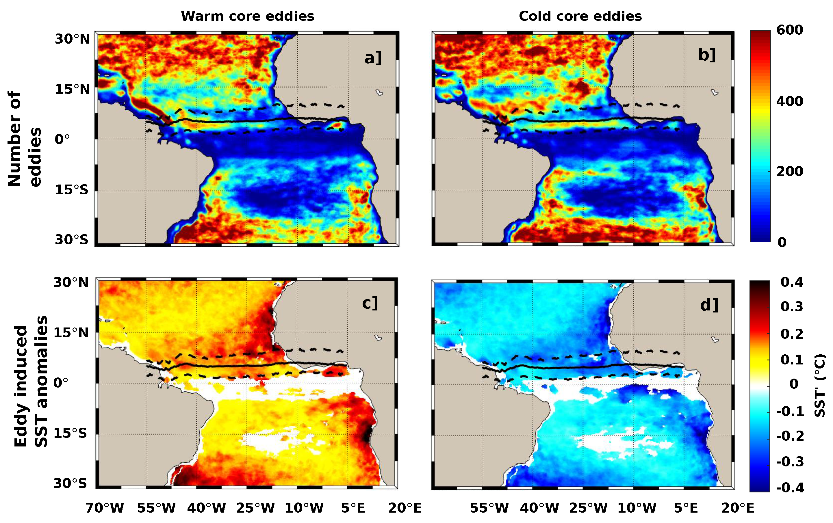
3.2.1. Spatial Distribution of Eddy-Induced SST Anomalies

On average, ∼60% of AEs and ∼40% of CEs have a positive SST anomaly, while the remaining ∼40% of AEs and ∼60% of CEs have a negative SST anomaly (

Table 1. Warm-core and cold-core eddies with their mean SST, LHF, SHF and IRF anomalies over 2010–2017 period.

	Cyclonic Eddies					Anticyclonic Eddies
	Number (%)	SST’ (°C)	LHF’ (W m−2)	SHF’ (W m−2)	IRF’ (W m−2)	Number (%)	SST’ (°C)	LHF’ (W m−2)	SHF’ (W m−2)	IRF’ (W m−2)
Warm-core eddies	145,868 (39.7%)	0.12 ± 0.05 *	1.5 ± 2.09	0.5 ± 0.60	0.73 ± 0.27	196,989 (59.8%)	0.16 ± 0.06	4.10 ± 2.27	1.15 ± 0.67	0.92 ± 0.33
Cold-core eddies	221,785 (60.3%)	−0.17 ± 0.08	−4.60 ± 2.14	−1.36 ± 0.63	−0.96 ± 0.40	132,231 (40.2%)	−0.13 ± 0.06	−2.78 ± 2.00	−0.80 ± 0.63	−0.79 ± 0.40
Total	367,653 (100%)	–	–	–	–	329,220 (100%)	–	–	–	–

* mean values ± one standard deviation.

). This suggests that AEs and CEs are not systematically warm-core or cold-core eddies, contrary to popular belief. However, the observed fraction of cold-core AEs and warm-core CEs in the TAO is higher than in the global ocean, where cold-core AEs and warm-core CEs account for about one-third of all eddies [32]. The spatial distributions of warm-core and cold-core eddies are comparable (Figure 6a,b). Eddy activities are most pronounced in the eastern and western boundaries, specifically in the eastern boundary upwelling systems (EBUS), along the southeastern coast of America, and north of 15°N and south of 20°S (Figure 6a,b). However, there are some regional differences, such as in the northern Hemisphere, south of 20°S and in SST frontal areas in the Cape Verde Frontal Zone (CVFZ) and in the Angola Benguela Frontal Zone (ABFZ). Indeed, in these regions, cold-core eddies slightly outnumber warm-core eddies with a maximum of 600 eddies per square degree. In the equatorial region, similarly to previous studies [1,5,6], the number of both warm-core and cold-core eddies is limited. However, a hot spot of both cold-core and warm-core eddies can be found beneath the ITCZ, between 40°W and 10°W longitude (Figure 6b), probably due to the zonal current instabilities, especially the North Equatorial Countercurrent, combined with equatorial upwelling which induces strong SST gradient. In the following, and for consistency, areas with a small number of eddies were discarded and were not taken into account in our analysis.

Figure 6c,d, displays the distribution of the mean eddy-induced SST anomalies in the TAO during the study period. In general, the distribution indicates low values of averaged eddy-induced SST anomalies of ±0.2 °C in the most areas. However, SST anomalies of ±0.4 °C are found in some regions such as in (i) the EBUS, (ii) the equatorial regions beneath the ITCZ, and (iii) southwest of the TAO off Brazil. There is also a hot spot of SST anomalies near the northern coast of the Gulf of Guinea. Despite these areas not being highly energetic in terms of EKE [1], they have a relatively high number of eddies (Figure 6a,b).

Despite the large number of warm-core CEs and cold-core AEs, the mean SST anomalies induced by all CEs (AEs respectively) remain dominantly negative (positive), reflecting what has been traditionnally admitted. In addition, the observed positive and negative anomalies witin all detected eddies do not cancel each other, highlithing the imprint of mesoscale eddies on SST in the TAO. On average, the ratio of the variance of eddy-induced SST anomalies to the total SST variability indicates that mesoscale eddies contribute to 10–25% oh the total SST variability in the TAO (not shown), with the maximum contribution observed beneath the ITCZ.

At the basin scale, eddy-induced SST anomalies exhibit no strong seasonal variability (not shown). However, in particular regions, mainly in the coastal and equatorial upwelling areas, a seasonal amplitude of eddy-induced SST anomalies up to 0.5 °C are observed. The seasonal amplitude is defined as the absolute difference of the maximum and minimum monthly anomalies.

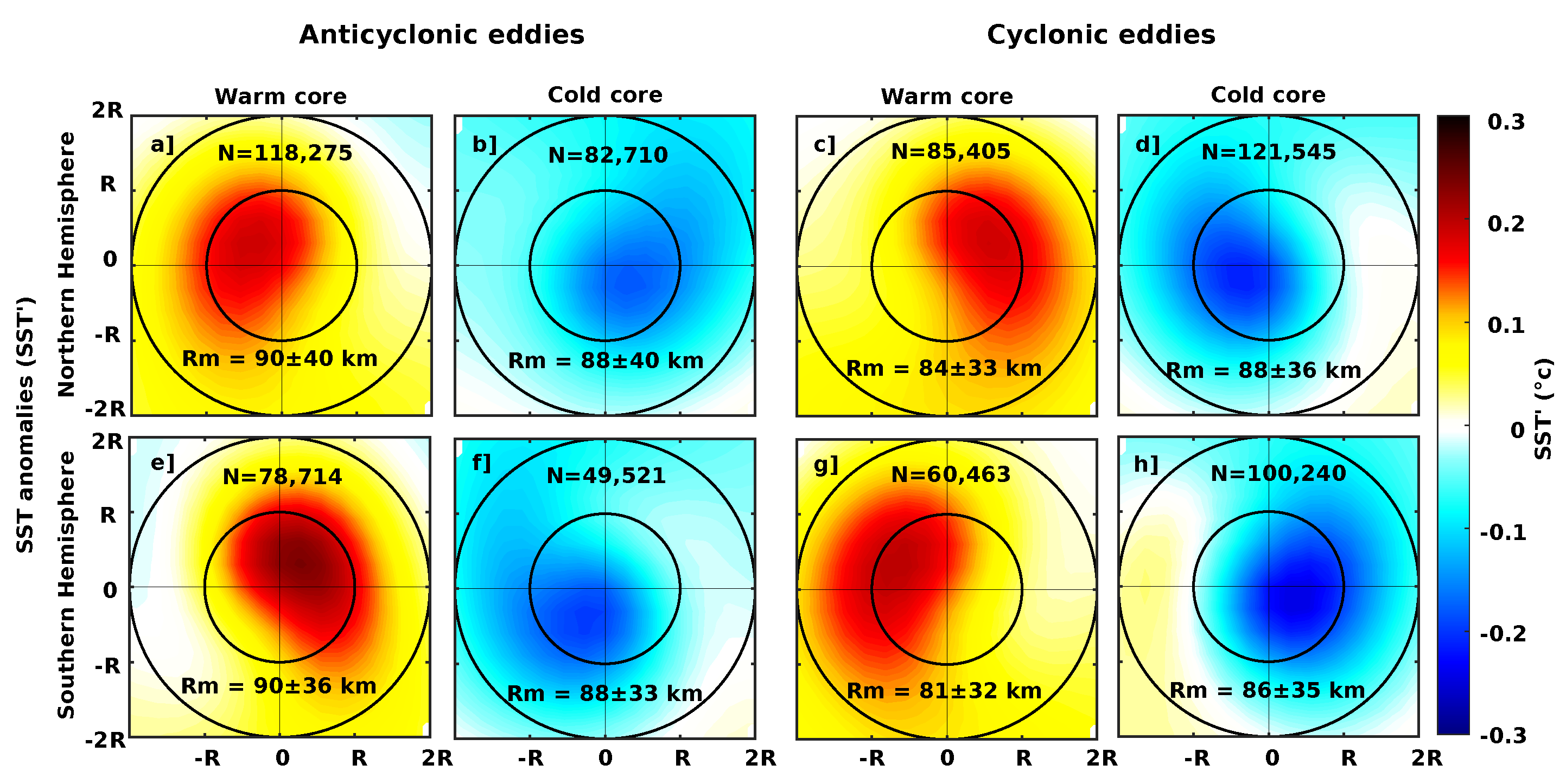
3.2.2. Composite Analysis of Eddy-Induced SST Anomalies

The composite analysis of eddy-induced SST anomalies was conducted in the Northern and Southern Hemispheres using the method outlined in Section 2. The results show that the maximum SST anomalies in both hemispheres are generally displaced from eddy centers and are closer to the edges (Figure 7). More precisely, in the Northern Hemisphere, maximum anomalies of about ±0.3 °C were found in the northwest quadrant for warm-core AEs and in the southeast quadrant for cold-core AEs (Figure 7a,b). AEs rotate clockwise in the Northern Hemisphere, and the mean large-scale SST gradient is southward-oriented in the rotated frame as shown by Figure 4a. This leads to the horizontal advection of warm SST from the south to the northwest and concurrently, cold SST from the north to the southeast. This mechanism of horizontal advection leads to positive SST anomalies in the northwest side of the eddies and negative SST anomalies in the southeast side. Similar processes have also been found to play a key role in eddy-induced SST, sea surface salinity and chlorophyll anomalies in some regional studies outside of the TAO [44,45,46,47]. In the Southern Hemisphere, maximum positive and negative SST anomalies were observed in opposite quadrants due to the anticlockwise rotation of AE (Figure 7e,f). Similar results were also obtained for CEs, but with opposite rotation direction in both hemispheres (Figure 7c,d,g,h).

Figure 8 shows the spatial distribution of axisymmetric and non-axisymmetric components of SST anomalies within AEs, averaged in 15° × 15° longitude/latitude subregions. Axisymmetric component distribution displays a similar pattern as the spatial distibution of mean SST anomalies (see Figure 6b,d), for both AEs and CEs (Figure 8a,b and Figure 9a,b). Stronger positive and negative composite anomalies are located along the eastern and southwestern boundaries of the TAO basin where coastal upwelling and where eddy activities are more intense. It is likely that these areas are favorable for vertical processes, basically because of uplifting/downlifting of isopycnal levels that occur inside eddies leading to cooling/warming of the ocean surface. In addition, as suggested by [33] in the Mediterranean Sea, vertical mixing modulation by eddies may also contribute in SST cooling and warming within AEs and CEs respectively, especially during spring and summer seasons. Moreover [21] demonstrated that AEs are more productive during winter due to the modulation of vertical mixing. Such a mechanism may lead to the cooling (warming) of SST witin AEs (CEs).

The non-axisymmetric components of SST anomalies are alsmost similar for both warm-core and cold-core AEs (Figure 8b,d). They are relatively weak, with average anomalies of around ±0.1 °C across the basin. However, certain areas, such as the ABFZ (near 10°E and 15°S) and the Cabo Frio Frontal Zone (CFFZ) (near 42°W and 23°S) display strong anomalies (Figure 8b,d) due to strong large-scale SST gradients as displayed in Figure 1. Likewise south of the equator and east of 25°W, where the seasonal Atlantic cold tong appears, causing a strong SST gradient, composite of SST anomalies are up to 0.2. Similar observations are valid for composite SST anomalies within CEs, as shown in Figure 9b,d. However, anomalies tend to be slightly higher compared with AEs non-axisymmetric composite, especially in high SST frontal areas.

3.2.3. Impact of Eddies on Latent Heat, Sensible Heat and Infrared Flux Anomalies

The spatial distribution of LHF, SHF and IRF anomalies within eddies is similar to that of SST anomalies. The maximum magnitude of the eddy-induced anomalies reaches up to ±10 W m⁻² for LHF, ±4 W m⁻² for SHF, and ±2 W m⁻² for IRF (Figure 10a–f), representing 10 to 35% of the heat fluxes variability. These results can be compared with previously studied regions of strong instabilities and high EKE, such as in the Agulhas Current retroflection, eddy-associated heat fluxes can reach ±20 W m⁻² [10]. Similarly, in the confluence of the Brazil–Malvinas confluence, LHF in some eddies can reach ±80 W m⁻² [34].

Eddy-induced heat flux anomalies are quasi-linear functions of eddy-induced SST anomalies (e.g., [48]) as shown by the bulk formulae relating LHF/SHF and SST (see Section 2). A relationship was established between eddy-induced SST anomalies and corresponding latent and sensible heat flux anomalies to better understand the coupling between SST and heat flux over eddies in the TAO. Eddy-induced SST anomalies were binned into 0.1 °C intervals, and the corresponding average heat flux anomalies were computed within each interval. As shown in Figure 11, significant linear relationships were observed between the eddy-induced SST and LHF/SHF anomalies, with correlation coefficients of 0.94 and 0.93, respectively. On average, the coupling strengths are ∼25 W m⁻² °C⁻¹ and ∼8 W m⁻² °C⁻¹ for LHF and SHF anomalies, respectively (Figure 11). However, it is important to note that heat fluxes are also influenced by other factors such as wind speed or the vertical temperature and moisture gradients between the ocean surface and the lower atmosphere (stratification). Additionally, the magnitude of heat fluxes over eddies are likely linked to eddy properties such as amplitude and radius, as previously reported by [10]. Larger amplitude eddies are generally associated with higher SST anomalies and stronger turbulent flux anomalies (not shown).

The LHF and SHF anomalies within eddies are proportional to the eddy-induced SST anomalies, resulting in similar spatial characteristics for composite averages of these heat flux anomalies (Figure 12) compared to those observed for SST anomalies (Figure 7). The highest heat-flux anomalies are observed close to eddy periphery with maximum values of ∼±8 W m⁻² and ∼±3 W m⁻² for LHF and SHF, respectively (Figure 12a–p).

3.3. Precipitation Anomalies over Eddies

The mean spatial structure of PR anomalies within eddies beneath the ITCZ and in the ∼10°W to 40°W longitude band differs from other regions in the TAO (Figure 13). PR Anomalies reach a maximum of ∼±2 mm day⁻¹ and represent ∼15–20% of daily mean PR (Figure 13a,b). There is a positive correlation between the PR and the turbulent heat flux anomalies, suggesting that increased (decreased) PR occurs over warm-core (cold-core) eddies (Figure 13a–c). However, the correlation coefficient found is relatively weak (|r| < 0.5), but with an average p-value of ∼0.05. In other areas of the TAO, no difference in the mean spatial distribution of PR between warm-core or cold-core eddies is observed (Figure 13a,b), with anomalies ranging by ±0.5 mm day⁻¹ and no significant correlation (|r| < 0.2; Figure 13c). This may be due to lower PR levels in these regions, which are generally 8 to 10 times lower than beneath the ITCZ (e.g., [49]).

4. Discussion

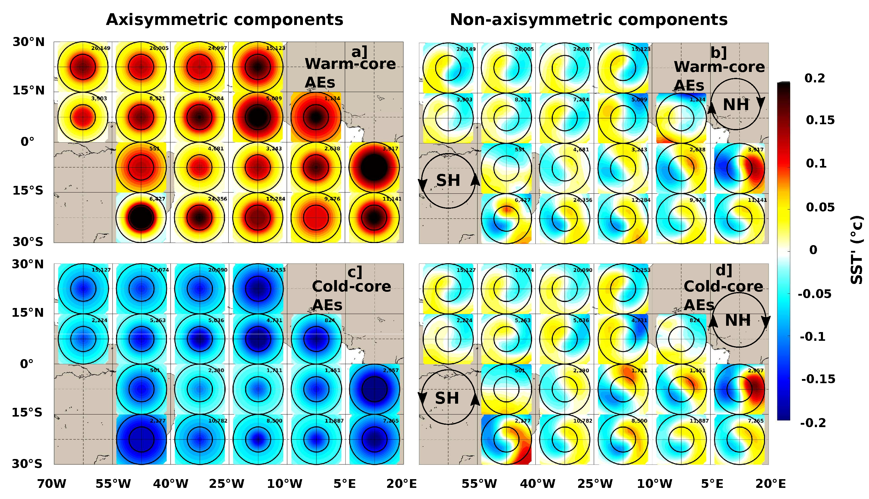
4.1. Contribution of Axisymmetric and Non-Axisymmetric Structures to Eddy Heat Flux

The results from Figure 8a,c and Figure 9a,c indicate net positive and negative SST anomalies within warm-core and cold-core eddies respectively, with high SST anomalies compared to the non-axisymmetric one. Even if the physical processes (including vertical mixing and advections) are complex to determine at this stage, these results suggest that axisymmetric components would have a greater impact on heat flux compared with non-axisymmetric components. Consequently, the non-axisymmetric components may not significantly contribute to the net LHF and SHF within eddies.

For evidence, the relationship between LHF and SHF anomalies have been reconstructed by considering only axisymmetric components of SST and heat flux anomalies, leading to similar relationships between heat flux anomalies and SST anomalies as observed in Figure 11. These results would suggest that, within the non-axisymmetric component, the upward heat fluxes are compensated by downward fluxes within the eddy interior as illustrated by Figure 14a). Contrastingly, the axisymmetric components are thought to be the main contributors to the net upward or downward heat fluxes within eddies, because of the one-way fluxes they induce (Figure 14b,c). These observations are also valid for the shortwave IRF anomalies, as IRF is a function of SST.

4.2. Relationship between Heat Flux and Precipitation Anomalies within Eddies

Despite the lower number of detected eddies near equatorial regions (Figure 4a,b), the ITCZ is characterized by a relatively high mean values of LHF and SHF anomalies within eddies. Moreover the fraction of the contribution of mesoscale activities relative to the totale variability was evaluated to 20–30%, highlighting the role that mesoscale eddies would play in the air–sea interaction and on cloud formation in the ITCZ. However, the ITCZ represents an area of high atmospheric convection processes and heavy precipitations area,thus, a high heat flux anomalies is expected and may explain the observed anomalies within eddies in this region.

Observations indicate that beneath the ITCZ, especially east of 35°W (see black box in Figure 12), higher positive PR anomalies within warm-core eddies are located south of ∼5°N (latitude of the mean location of the ITCZ), while within cold-core eddies, higher negative PR anomalies are almost centered on the ITCZ, extending from ∼5°N to ∼8°N (Figure 12a,b). As shown by the correlation between the total heat flux and PR anomalies (Figure 12c), the observed PR anomalies corroborated well with the SHF and LHF anomalies in the defined area. Indeed, SHF and LHF anomalies within warm-core edddies are relatively higher south of the mean location of the ITCZ, compared with anomalies in the northern part (Figure 9a,c). In contrast, within cold-core eddies, negative PR anomalies are almost centered on the mean location of the ITCZ (Figure 9b,d), highlighting the influence that eddies might have on PR in this area. This correlation is weak (between ∼2 and 8°N), but significant (p-value ≈ 0.05). The observed weak correlations might be explained by the fact that evaporation and PR processes do not occur instantly in space and time, particularly beneath the ITCZ, where higher heat flux and PR anomalies are observed. Indeed, the propagation of eddies, coupled with the displacement of atmospheric air masses and precipitating clouds, can induce a potential spatio-temporal phase shift between the eddy signature on heat fluxes and PR. It is likely that excessive heat release from a warm-core eddy leads to cloud formation and PR outside of the eddy. Another potential reason could be the low eddy activity that characterizes near equatorial regions such as the TAO, compared to mid- and high-latitude regions where eddy activities are more intense [1,5,50,51].

The strong positive PR anomalies observed in the ∼2–5°N latitude band seem to appear seasonally. Indeed, the seasonal variation reveals that positive PR anomalies within eddies are maximum during boreal winter (not shown). Since the ITCZ is at its southernmost latitudes (between 2 and 5°N) during this period of the year [52], the observed PR maximum anomalies within eddies might possibly be influenced by the induced heavy PR. In addition, the seasonal variation of SST gradient due to atmospheric and oceanic processes such as trade winds and equatorial upwelling [53], might also have an influence on the eddy-induced SST anomalies and thus on the heat fluxes and PR anomalies. Analysis of such processes is beyond the scope of this study but are of a great interest for future studies, especially using modeling.

5. Conclusions

Combining 8 years of daily altimetry ADT, SST, LHF, SHF, ocean IRF and PR data, this study aimed to investigate the influence of mesoscale eddies on air–sea heat exchange in the TAO, and the relationship between heat flux and PR anomalies over eddies. Results indicated that in the TAO, about 40% of the CEs are warm-core CEs and 40% of AEs are cold-core AEs. Eddy-induced SST anomalies ranged between ±0.4 °C, contributing to 10–25% of the total SST variability in the TAO, with higher anomalies observed in coastal regions, especially EBUS.

Heat flux anomalies over eddies showed patterns similar to SST anomalies, with maximum positive and negative values of ±10 W m⁻² for LHF, ±4 W m⁻² for SHF, and ±2 W m⁻² for IRF. The eddy-associated anomalies accounted for 10–35% of the LHF and SHF variability. On average, LHF and SHF anomalies over eddies varied quasi-linearly with eddy-induced SST anomalies, with coupling strength coefficients of ∼25 and ∼8 W m⁻² °C⁻¹, respectively. Composite anomalies were constructed and decomposed into axisymmetric and non-axisymmetric components. Only the axisymmetric part of eddy-induced SST anomalies were found to significantly influence the net LHF, SHF and IRF over eddies.

The PR anomalies over eddies are significant only beneath the ITCZ, with values up to ∼±2 mm day⁻¹. The correlation between heat flux et PR anomalies are relatively weak but significant, probably because of the differences of spatial and temporal scale of atmospheric and oceanic mesoscale processes. Investigations of the impact of such difference and the atmospheric responses in wind speed and cloud formation could be set up from a high resolution numerical coupled ocean-atmosphere model, and will deserve future studies. Moreover, PR, as a freshwater flux, is known to be the main driver of large-scale salinity changes in the equatorial Atlantic beneath the ITCZ [54]. However, the role of mesoscale eddies in salinity variability in the near-equatorial region, beneath the ITCZ is not well understood. Investigating the influence of mesoscale eddies in this context would deepen our understanding of the mesoscale physical processes influence in salinity changes in the equatorial Atlantic.

References

1. Aguedjou, H.M.A.; Dadou, I.; Chaigneau, A.; Morel, Y.; Alory, G. Eddies in the Tropical Atlantic Ocean and Their Seasonal Variability. Geophys. Res. Lett. 2019, 46, 12156–12164. [Google Scholar] [CrossRef]
2. Chaigneau, A.; Gizolme, A.; Grados, C. Mesoscale eddies off Peru in altimeter records: Identification algorithms and eddy spatio-temporal patterns. Prog. Oceanogr. 2008, 79, 106–119. [Google Scholar] [CrossRef]
3. Chaigneau, A.; Eldin, G.; Dewitte, B. Eddy activity in the four major upwelling systems from satellite altimetry (1992–2007). Prog. Oceanogr. 2009, 83, 117–123. [Google Scholar] [CrossRef]
4. Chelton, D.B.; Schlax, M.G.; Samelson, R.M.; de Szoeke, R.A. Global observations of large oceanic eddies. Geophys. Res. Lett. 2007, 34. [Google Scholar] [CrossRef]
5. Chelton, D.B.; Schlax, M.G.; Samelson, R.M. Global observations of nonlinear mesoscale eddies. Fluids 2011, 91, 167–216. [Google Scholar] [CrossRef]
6. Fu, L.-L.; Chelton, D.; Le Traon, P.-Y.; Morrow, R. Eddy Dynamics From Satellite Altimetry. Oceanography 2011, 23, 14–25. [Google Scholar] [CrossRef]
7. Laxenaire, R.; Speich, S.; Blanke, B.; Chaigneau, A.; Pegliasco, C.; Stegner, A. Anticyclonic Eddies Connecting the Western Boundaries of Indian and Atlantic Oceans. J. Geophys. Res. Ocean. 2018, 123, 7651–7677. [Google Scholar] [CrossRef]
8. Pegliasco, C.; Chaigneau, A.; Morrow, R. Main eddy vertical structures observed in the four major Eastern Boundary Upwelling Systems. J. Geophys. Res. Ocean. 2015, 120, 6008–6033. [Google Scholar] [CrossRef]
9. Chu, X.; Xue, H.; Qi, Y.; Chen, G.; Mao, Q.; Wang, D.; Chai, F. An exceptional anticyclonic eddy in the South China Sea in 2010. J. Geophys. Res. Ocean. 2014, 119, 881–897. [Google Scholar] [CrossRef]
10. Villas Bôas, A.B.; Sato, O.T.; Chaigneau, A.; Castelão, G.P. The signature of mesoscale eddies on the air-sea turbulent heat fluxes in the South Atlantic Ocean. Geophys. Res. Lett. 2015, 42, 1856–1862. [Google Scholar] [CrossRef]
11. Yang, P.; Jing, Z.; Wu, L. An Assessment of Representation of Oceanic Mesoscale Eddy-Atmosphere Interaction in the Current Generation of General Circulation Models and Reanalyses. Geophys. Res. Lett. 2018, 45, 11856–11865. [Google Scholar] [CrossRef]
12. Wang, D.X.; Xu, H.Z.; Lin, J.; Hu, J.Y. Anticyclonic eddies in the northeastern South China Sea during winter 2003/2004. J. Oceanogr. 2008, 64, 925–935. [Google Scholar] [CrossRef]
13. Aguedjou, H.M.A.; Chaigneau, A.; Dadou, I.; Morel, Y.; Pegliasco, C.; Da-Allada, C.Y.; Baloïtcha, E. What Can We Learn From Observed Temperature and Salinity Isopycnal Anomalies at Eddy Generation Sites? Application in the Tropical Atlantic Ocean. J. Geophys. Res. Ocean. 2021, 126, 1–27. [Google Scholar] [CrossRef]
14. Chaigneau, A.; Le Texier, M.; Eldin, G.; Grados, C.; Pizarro, O. Vertical structure of mesoscale eddies in the eastern South Pacific Ocean: A composite analysis from altimetry and Argo profiling floats. J. Geophys. Res. Ocean. 2011, 116. [Google Scholar] [CrossRef]
15. Keppler, L.; Cravatte, S.; Chaigneau, A.; Pegliasco, C.; Gourdeau, L.; Singh, A. Observed Characteristics and Vertical Structure of Mesoscale Eddies in the Southwest Tropical Pacific. J. Geophys. Res. Ocean. 2018, 123, 2731–2756. [Google Scholar] [CrossRef]
16. Sandalyuk, N.V.; Belonenko, T.V. Three-dimensional structure of the mesoscale eddies in the Agulhas Current region from hydrological and altimetry data. Russ. J. Earth Sci. 2021, 21, 1–19. [Google Scholar] [CrossRef]
17. Schütte, F.; Brandt, P.; Karstensen, J. Occurrence and characteristics of mesoscale eddies in the tropical northeastern Atlantic Ocean. Ocean. Sci. 2016, 12, 663–685. [Google Scholar] [CrossRef]
18. Sun, W.; Dong, C.; Tan, W.; Liu, Y.; He, Y.; Wang, J. Vertical structure anomalies of oceanic eddies and eddy-induced transports in the South China Sea. Remote Sens. 2018, 10, 795. [Google Scholar] [CrossRef]
19. Zhang, Z.; Zhao, W.; Tian, J.; Liang, X. A mesoscale eddy pair southwest of Taiwan and its influence on deep circulation. J. Geophys. Res. 2013, 118, 6479–6494. [Google Scholar] [CrossRef]
20. Dadou, I.; Garçon, V.; Andersen, V.; Flierl, G.R.; Davis, C.S. Impact of the North Equatorial Current meandering on a pelagic ecosystem: A modeling approach. J. Mar. Res. 1996, 54, 311–342. [Google Scholar] [CrossRef]
21. Dufois, F.; Hardman-Mountford, N.J.; Greenwood, J.; Richardson, A.J.; Feng, M.; Matear, R.J. Anticyclonic eddies are more productive than cyclonic eddies in subtropical gyres because of winter mixing. Sci. Adv. 2016, 2, e1600282. [Google Scholar] [CrossRef]
22. Mcgillicuddy, D.J., Jr. Mechanisms of Physical- Biological-Biogeochemical Interaction at the Oceanic Mesoscale. Annu. Rev. Mar. Sci. 2016, 8, 125–159. [Google Scholar] [CrossRef] [PubMed]
23. Chen, G.; Wang, Q.; Chu, X. Accelerated spread of Fukushima’s waste water by ocean circulation. Innovation 2021, 2, 100119. [Google Scholar] [CrossRef] [PubMed]
24. Chelton, D.B.; Xie, S.P. Coupled ocean-atmosphere interaction at oceanic mesoscales. Oceanography 2010, 23, 54–69. [Google Scholar] [CrossRef]
25. Frenger, I.; Gruber, N.; Knutti, R.; Münnich, M. Imprint of Southern Ocean eddies on winds, clouds and rainfall. Nat. Geosci. 2013, 6, 608–612. [Google Scholar] [CrossRef]
26. Carton, J.A.; Chepurin, G.A.; Ligan, C.; Grodsky, S.A. Improved Global Net Surface Heat Flux. J. Geophys. Res. Ocean. 2018, 123, 3144–3163. [Google Scholar] [CrossRef]
27. Adam, O.; Bischoff, T.; Schneider, T. Seasonal and interannual variations of the energy flux equator and ITCZ. Part II: Zonally varying shifts of the ITCZ. J. Clim. 2016, 29, 7281–7293. [Google Scholar] [CrossRef]
28. Eichhorn, A.; Bader, J. Impact of tropical Atlantic sea-surface temperature biases on the simulated atmospheric circulation and precipitation over the Atlantic region: An ECHAM6 model study. Clim. Dyn. 2017, 49, 2061–2075. [Google Scholar] [CrossRef]
29. Xie, S.; Carton, J.A. Tropical Atlantic Variability: Patterns, Mechanisms, and Impacts. Earth Clim. Ocean.-Atmos. Interact. 2004, 147, 121–142. [Google Scholar]
30. Farneti, R.; Stiz, A.; Ssebandeke, J.B. Improvements and persistent biases in the southeast tropical Atlantic in CMIP models. NPJ Clim. Atmos. Sci. 2022, 5, 42. [Google Scholar] [CrossRef]
31. Assassi, C.; Morel, Y.V.; Ermeirsch, F.; Chaigneau, A.; Pegliasco, C.; Morrow, R.; Colas, F.; Fleury, S.; Carton, X.; Klein, P.; et al. An index to distinguish surface- and subsurface-intensified vortices from surface observations. J. Phys. Oceanogr. 2016, 46, 2529–2552. [Google Scholar] [CrossRef]
32. Liu, Y.; Zheng, Q.; Li, X. Characteristics of Global Ocean Abnormal Mesoscale Eddies Derived From the Fusion of Sea Surface Height and Temperature Data by Deep Learning. Geophys. Res. Lett. 2021, 48, e2021GL094772. [Google Scholar] [CrossRef]
33. Moschos, E.; Barboni, A.; Stegner, A. Why Do Inverse Eddy Surface Temperature Anomalies Emerge? The Case of the Mediterranean Sea. Remote Sens. 2022, 14, 3807. [Google Scholar] [CrossRef]
34. Leyba, I.M.; Saraceno, M.; Solman, S.A. Air-sea heat fluxes associated to mesoscale eddies in the Southwestern Atlantic Ocean and their dependence on different regional conditions. Clim. Dyn. 2016, 49, 2491–2501. [Google Scholar] [CrossRef]
35. Sun, W.; Dong, C.; Tan, W.; He, Y. Statistical characteristics of cyclonic warm-core eddies and anticyclonic cold-core eddies in the North Pacific based on remote sensing data. Remote Sens. 2019, 11, 208. [Google Scholar] [CrossRef]
36. Pujol, M.I.; Faugère, Y.; Taburet, G.; Dupuy, S.; Pelloquin, C.; Ablain, M.; Picot, N. DUACS DT2014: The new multi-mission altimeter data set reprocessed over 20 years. Ocean. Sci. 2016, 12, 1067–1090. [Google Scholar] [CrossRef]
37. Huang, B.; Liu, C.; Banzon, V.; Freeman, E.; Graham, G.; Hankins, B.; Smith, T.; Zhang, H.M. Improvements of the Daily Optimum Interpolation Sea Surface Temperature (DOISST) Version 2.1. J. Clim. 2021, 34, 2923–2939. [Google Scholar] [CrossRef]
38. Reynolds, R.W.; Smith, T.M.; Liu, C.; Chelton, D.B.; Casey, K.S.; Schlax, M.G. Daily high-resolution-blended analyses for sea surface temperature. J. Clim. 2021, 20, 5473–5496. [Google Scholar] [CrossRef]
39. Bentamy, A.; Grodsky, S.A.; Katsaros, K.B.; Mestas-Nuñez, A.M.; Blanke, B.; Desbiolles, F. Improvement in air–sea flux estimates derived from satellite observations. Int. J. Remote Sens. 2013, 34, 5243–5261. [Google Scholar] [CrossRef]
40. Bentamy, A.; Grodsky, S.A.; Elyouncha, A.; Chapron, B.; Desbiolles, F. Homogenization of scatterometer wind retrievals. Int. J. Climatol. 2016, 37, 870–889. [Google Scholar] [CrossRef]
41. Bentamy, A.; Piolle, J.F.; Grouazel, A.; Danielson, R.; Gulev, S.; Paul, F.; Azelmat, H.; Mathieu, P.P.; von Schuckmann, K.; Sathyendranath, S.; et al. Review and assessment of latent and sensible heat fl ux accuracy over the global oceans. Remote Sens. Environ. 2017, 201, 196–218. [Google Scholar] [CrossRef]
42. Huffman, G.J.; Adler, R.F.; Arkin, P.; Chang, A.; Ferraro, R.; Gruber, A.; Janowiak, J.; McNab, A.; Rudolf, B.; Schneider, U. The Global Precipitation Climatology Project (GPCP) Combined Precipitation Dataset. Bull. Am. Meteorol. Soc. 1997, 78, 5–20. [Google Scholar] [CrossRef]
43. Huffman, G.J.; Adler, R.F.; Bolvin, D.T.; Nelkin, E.J. The TRMM Multi-Satellite Precipitation Analysis (TMPA). In Satellite Rainfall Applications for Surface Hydrology; Springer: Berlin/Heidelberg, Germany, 2010; pp. 3–22. [Google Scholar]
44. Delcroix, T.; Chaigneau, A.; Soviadan, D.; Boutin, J.; Pegliasco, C. Eddy-Induced Salinity Changes in the Tropical Pacific. J. Geophys. Res. Ocean. 2019, 124, 374–389. [Google Scholar] [CrossRef]
45. Gaube, P.; Chelton, D.B.; Samelson, R.M.; Schlax, M.G.; O’Neill, L.W. Satellite observations of mesoscale eddy-induced Ekman pumping. J. Phys. Oceanogr. 2015, 45, 104–132. [Google Scholar] [CrossRef]
46. Chelton, D.B.; Gaube, P.; Schlax, M.G.; Early, J.J.; Samelson, R.M. The Influence of Nonlinear Mesoscale Eddies on Near-Surface Oceanic Chlorophyll. Science 2011, 334, 328–333. [Google Scholar] [CrossRef]
47. Gaube, P.; McGillicuddy, D.J.; Chelton, D.B.; Behrenfeld, M.J.; Strutton, P.G. Regional variations in the influence of mesoscale eddies on near-surface chlorophyll. J. Geophys. Res. Ocean. 2014, 119, 8195–8220. [Google Scholar] [CrossRef]
48. Liu, Y.; Yu, L.; Chen, G. Characterization of Sea Surface Temperature and Air-Sea Heat Flux Anomalies Associated with Mesoscale Eddies in the South China Sea. J. Geophys. Res. Ocean. 2020, 125, e2019JC015470. [Google Scholar] [CrossRef]
49. Liu, X.; Chang, P.; Kurian, J.; Saravanan, R.; Lin, X. Satellite-observed precipitation response to ocean mesoscale eddies. J. Clim. 2018, 31, 6879–6895. [Google Scholar] [CrossRef]
50. Greaser, S.R.; Subrahmanyam, B.; Trott, C.B.; Roman-Stork, H.L. Interactions Between Mesoscale Eddies and Synoptic Oscillations in the Bay of Bengal During the Strong Monsoon of 2019. J. Geophys. Res. Ocean. 2020, 125, 1–29. [Google Scholar] [CrossRef]
51. Trott, C.B.; Subrahmanyam, B.; Chaigneau, A.; Delcroix, T. Eddy Tracking in the Northwestern Indian Ocean During Southwest Monsoon Regimes. Geophys. Res. Lett. 2018, 45, 6594–6603. [Google Scholar] [CrossRef]
52. Nnamchi, H.C.; Latif1, M.; Keenlyside, N.S.; Kjellsson, J.; Richter, I. Diabatic heating governs the seasonality of the Atlantic Niño. Nat. Commun. 2021, 12, 376. [Google Scholar] [CrossRef] [PubMed]
53. Helber, R.W.; Weisberg, R.H.; Bonjean, F.; Johnson, E.S.; Lagerloef, G.S.E. Satellite-derived surface current divergence in relation to tropical Atlantic SST and wind. Am. Meteorol. Soc. 2006, 37, 1357–1375. [Google Scholar] [CrossRef]
54. Da-Allada, C.Y.; Alory, G.; Du Penhoat, Y.; Kestenare, E.; Dur, F.; Hounkonnou, N.M. Seasonal mixed-layer salinity balance in the tropical Atlantic Ocean: Mean state and seasonal cycle. J. Geophys. Res. Ocean. 2013, 118, 332–345. [Google Scholar] [CrossRef]
Figure 1. Mean sea surface temperature (SST, background color) and SST gradient (black thin contour lines) in the tropical Atlantic ocean (TAO) from 2010 to 2017. The green thick solid and dashed lines denote the average and the northernmost and southernmost locations of the intertropical convergence zone (ITCZ), during boreal winter and summer, respectively. Magenta dashed lines represent Cape Verde Frontal Zone, Angola Benguela Frontal and Cabo Frio Frontal. North Brazil Current Retroflection (NBCR), North Equatorial Current (NEC), North Equatorial Counter-current (NECC), Brazil Current (BC), Angola Current (AC) and Benguela Current (BeC) are shown by wide black arrows.
Remotesensing 15 03087 g001
Figure 2. High-pass filtered SST (background color) and detected eddies on 25 November 2012. Cyclonic and anticyclonic eddy edges are represented in thick and thin black contours, respectively.
Remotesensing 15 03087 g002
Figure 3. (a) A representative example of an eddy with its central core, where the mean anomalies were computed. (b,c) Mean SST anomalies induced by warm-core and cold-core eddies on 25 November 2012. White areas are areas without eddies.
Remotesensing 15 03087 g003
Figure 4. (a) Example of large-scale SST pattern within an eddy after rotation in a normalized coordinate system. (b) Composite of SST anomalies within eddy with corresponding (c) non-axisymmetric and (d) axisymmetric component. Surface geostrophic currents are represented by black arrows. R denotes the eddy radius.
Remotesensing 15 03087 g004
Figure 5. Histograms of eddy (a) amplitude, (b) kinetic energy, (c) radius and (d) lifespan in the TAO.
Remotesensing 15 03087 g005
Figure 6. Distribution of (a,b) warm-core and cold-core eddies, and (c,d) eddy-induced SST anomalies over the 2010–2017 period. Solid and dashed curves represent the mean annual and extreme (during boreal winter and summer) location of the ITCZ. White areas stand for areas where not enough eddies were available.
Remotesensing 15 03087 g006
Figure 7. Averaged composites of SST anomalies within warm-core and cold-core (a,b,e,f) anticyclonic and (c,d,g,h) cyclonic eddies in the Northern and Southern Hemisphere. For each composite, N denotes the number of individual eddy while Rm denotes their mean radius ± one standard deviation.
Remotesensing 15 03087 g007
Figure 8. Distribution of (a,c) axisymmetric and (b,d) non-axisymmetric component of warm-core and cold-core anticyclonic eddies. Rotation direction of eddies are indicated in the Northern and Southern Hemisphere on black circles.
Remotesensing 15 03087 g008
Figure 9. Distribution of (a,c) axisymmetric and (b,d) non-axisymmetric component of warm-core and cold-core cyclonic eddies. Rotation direction of eddies are indicated in the Northern and Southern Hemisphere on black circles.
Remotesensing 15 03087 g009
Figure 10. Distribution of (a,b) latent heat flux (LHF), (c,d) sensible heat flux (SHF) and (e,f) ocean infrared flux (IRF) anomalies over warm-core and cold-core eddies. Solid and dashed curves represent the mean annual and extreme (during boreal winter and summer) location of the ITCZ.
Remotesensing 15 03087 g010
Figure 11. Eddy-induced heat flux anomalies as function of SST anomalies (black dots) with the corresponding linear fitting for LHF (magenta full line) and SHF (green full line) anomalies. Dashed lines indicate the linear fitting obtained when considering only the axisymmetric components of composites of SST and heat flux anomalies (see text). Error bars denote ±1 standard deviation.
Remotesensing 15 03087 g011
Figure 12. Same as Figure 5 for (ah) latent and (ip) sensible heat flux anomalies. The number of average eddy composites is denoted N.
Remotesensing 15 03087 g012
Figure 13. Mean spatial distribution of PR anomalies over (a) warm-core and (b) cold-core eddies and (c) correlation coefficient between heat flux and PR anomalies.
Remotesensing 15 03087 g013
Figure 14. Schematic representation of the contribution of (a) non-axisymmetric and (b,c) axisymmetric components to the net latent and sensible heat fluxes. The considered eddy in (a) has a counterclockwise rotation direction.
Remotesensing 15 03087 g014