Object-Oriented Clustering Approach to Detect Evolutions of ENSO-Related Precipitation Anomalies over Tropical Pacific Using Remote Sensing Products

Abstract

Precipitation extremes driven by the El Niño–Southern Oscillation (ENSO) are one of the critical ways in which the ENSO impacts the global climate, specifically in the tropical Pacific, where they have the potential to cause extreme weather conditions. However, existing approaches struggle to effectively identify the evolution of ENSO-related precipitation anomalies that change rapidly in spatial distribution. To address this challenge, we propose the object-oriented spatiotemporal clustering approach using remote sensing products (OSCAR) for detecting evolutions of ENSO-related precipitation anomalies. The OSCAR was validated using simulated datasets and applied to precipitation anomalies over the tropical Pacific. The simulation experiment demonstrates that the OSCAR outperforms the dual-constraint spatiotemporal clustering approach (DcSTCA) in accuracy, particularly for rapidly evolving precipitation anomaly variations. The application of the OSCAR demonstrates its ability to recognize the evolution of ENSO-related precipitation anomalies over the tropical Pacific, which may offer valuable references for global climate change research.

1. Introduction

The El Niño–Southern Oscillation (ENSO) is an interannual phenomenon characterized by sea surface temperatures and convection anomalies in the tropical Pacific [1,2,3]. Precipitation extremes driven by the ENSO are a crucial pathway through which the ENSO affects the global climate [4]. ENSO-driven tropical Pacific precipitation, anticipated to be amplified due to surface warming [4,5,6], can result in extreme weather events worldwide, causing significant damage to agriculture, ecosystems, and the economy [7,8,9]. Precipitation is not only driven by the ENSO, but it also has the potential to influence ENSO in reverse. The precipitation–SST feedback loop, which plays a vital role in ENSO development, can significantly modulate the ENSO’s properties by affecting sea surface salinity, mixed-layer depth, and the ocean barrier layer [10,11,12,13,14,15,16].

Thanks to the advances in remote sensing technology, numerous remote sensing products offer long-term series of historical data for analyzing global climate change, including changes in precipitation [17]. Pike and Lintner utilized the K-means clustering approach to identify characteristic spatial patterns of precipitation over the South Pacific convergence zone (SPCZ) and analyzed the relationship between the spatial pattern of precipitation and ENSO phases [18]. Wang et al. discussed the robustness of the relationship between precipitation in Asia and the ENSO [19]. Ma et al. studied the mechanisms of the ENSO’s impact on precipitation anomalies in East Asia during early winter [20]. The previous studies mainly focus on the overall spatial patterns of precipitation statistics during various periods in the study area rather than the spatiotemporal dynamic evolution of precipitation from its inception to development and dissipation.

To track the evolution of storms, Dixon and Wiener introduced the thunderstorm identification, tracking, analysis, and nowcasting (TITAN) methodology utilizing radar data [21]. The limitation of TITAN is that it only considers a few factors when identifying and tracking rainstorm events, and these factors are not comprehensive enough [22,23]. Several modifications to two aspects of this methodology have been proposed to overcome this limitation: identification and tracking. To improve rainstorm identification, multiple thresholds and spatiotemporal features have been employed to discern different types of rainstorms [22,23,24,25,26]. To improve the tracking of rainstorms, several modifications have been introduced. For example, Liu et al. distinguished rainstorm events based on overlap area, centroid distance, and velocity direction [25]. Muñoz et al. integrated an optical-flow field tracker to enhance the matching of rainstorms at successive timestamps [23]. Hou and Wang designed a tree structure model of a rainstorm to represent the intensity regions in radar images and their spatial relationships [27]. Xue et al. proposed a process-oriented algorithm for identifying and tracking rainstorms that outperforms the TITAN algorithm [28]. These identification and tracking methods are specific to rainstorm events and are usually applied to precipitation data with temporal resolutions higher than the hour. Hence, these methods are not suitable for the spatiotemporal clustering of ENSO-related precipitation anomalies with monthly scales.

In order to identify the spatiotemporal patterns of variations in marine anomalies, Liu et al. proposed a dual-constraint spatiotemporal clustering approach (DcSTCA) and applied it to ENSO-related monthly SST [29]. Since the basic clustering unit of DcSTCA is the pixel, it struggles to accurately capture the evolution process of marine anomalies that change rapidly in the spatial range, resulting in missed pixels at timestamps of sudden change. Depending on the spatiotemporal clusters produced by the DcSTCA, Li et al. and Xue et al. abstracted cluster profiles at each timestamp into snapshot objects and reorganized them based on overlapping or morphological features to reconstruct and optimize the evolutionary structure of clusters [30,31]. Nonetheless, as the snapshot objects are still derived from the DcSTCA, these methods remain ineffective at detecting the rapidly changing variations in marine anomalies.

To address this limitation, we propose an object-oriented spatiotemporal clustering approach using remote sensing products (OSCAR) that uses snapshot objects as the basic clustering unit. The OSCAR was validated using simulated datasets and applied to detect the evolutions of ENSO-related precipitation anomalies in the tropical Pacific from long-term remote sensing products. The relationship between these precipitation evolutions and the ENSO’s development was then analyzed.

2. Materials and Methods

2.1. Materials

2.1.1. Simulated Raster Dataset

To validate the efficacy and accuracy of the OSCAR, a simulated dataset of precipitation anomalies was generated, encompassing 10 consecutive timestamps from 1 to 10, with each timestamp featuring a raster size of 60 × 20, as shown in Figure 1. In this figure, the dark-colored regions signify precipitation anomalies, while the light-colored regions represent the background. The attribute values of the background pixels are not unique values but rather random values that follow a normal distribution with a mean of 0 and a variance of 1. Additionally, noisy pixels with similar attribute values to the precipitation anomalies were inserted to the background. The aim is to enhance the similarity between the simulated dataset and the actual remote sensing products, thereby validating the spatiotemporal clustering of precipitation anomalies accurately.

Precipitation anomalies may expand, narrow, move, merge, and split during their evolution, which is a challenging problem in the spatiotemporal clustering of these variations. Based on these evolutionary behaviors, the evolutionary processes of precipitation anomalies were designed in the simulated dataset. The simulated dataset comprised three evolutionary processes, A, B, and C, representing the expansion and narrowing, movement, and merging and splitting behaviors of precipitation anomalies variations, respectively. Process A initially expanded and then reduced, reaching its maximum area at timestamp 5. Process B’s overall trend was moving from left to right with varying speeds. The movement speed was slow between timestamp 4 and 6 and comparatively faster between timestamp 7 and 10. Process C showed merging at timestamp 3 and splitting at timestamp 8. The objective of the simulation experiment was to evaluate the capability of the OSCAR to recognize development, movement, splitting, and merging evolution processes.

2.1.2. Remote Sensing Products

Integrated Multi-Satellite Retrievals for GPM (IMERG) is a data fusion method within the Global Precipitation Measurement (GPM) project that globally calibrates, combines, and interpolates data from all microwave satellite precipitation, infrared satellite precipitation, and other precipitation data sources. The IMERG-Final Run is the research-quality data series within IMERG, commencing from June 2000.

In this study, the rasters of IMERG-Final Run were resampled to 1° × 1° pixels. As the monthly oscillations of precipitation obscure the annual oscillations induced by ENSO events, we applied the monthly standardized anomaly to each pixel to remove the monthly oscillations, as presented in Equation (1):

$$X_{t,m}^{\prime }=\frac{X_{t,m}-{\overline{X}}_m}{{\delta }_m}$$

(1)

In the formula, m is the month, such as January or February; t is the timestamp, such as January 2020 or February 2020; ${\overline{X}}_m$ is the average value of month m; and ${\delta }_m$ is the standard deviation of month m.

The bi-monthly multivariate ENSO index (MEI) is utilized as an indicator of ENSO event strength to analyze the relationship between the ENSO and tropical Pacific precipitation anomalies. The MEI index was derived from five factors: sea level pressure, sea surface temperature, zonal and meridional components of surface wind, and outgoing longwave radiation [32]. To account for the ENSO’s seasonality and minimize the impact of intraseasonal variability, the MEI index was calculated for 12 overlapping bi-monthly “seasons,” such as December–January, January–February, etc. Based on the MEI index, McPhaden et al. defined El Niño events as periods when the MEI index remains above 0.5 for at least five consecutive months, while La Niña events are periods with an MEI index below −0.5 [2].

2.2. Methods

An object-oriented spatiotemporal clustering approach, called OSCAR, was proposed to detect the evolution of variations in precipitation anomalies. This method first identifies the snapshot objects from the raster of remote sensing products, representing the status of the precipitation anomaly, and then performs spatiotemporal clustering on the snapshot objects, as shown in Figure 2.

The parameters of the OSCAR are density threshold K, attribute threshold Kth, and overlapping threshold θ, corresponding to temporal, spatial, and attribute similarities, respectively, for clustering. Definitions of related concepts are as follows.

• Spatial Neighborhood: The spatial neighborhood of a pixel is the other eight surrounding pixels.
• Core Pixel: For a pixel p, if the number of neighboring pixels with attribute distance from p less than Kth is fewer than K in p’s spatial neighborhood, then p is the core pixel.
• Reachable Pixel: A pixel is considered reachable for a cluster when the difference between its attribute and the average attribute of the cluster does not exceed Kth.
• Isolated Pixel: Isolated pixels are reachable pixels situated at the corners of the spatial neighborhood that are not adjacent to other reachable pixels.
• Merge: Multiple snapshot objects at a given timestamp are overlapping with and similar to a snapshot object from the subsequent timestamp.
• Split: Multiple snapshot objects at a given timestamp are overlapping with and similar to a snapshot object from the previous timestamp.

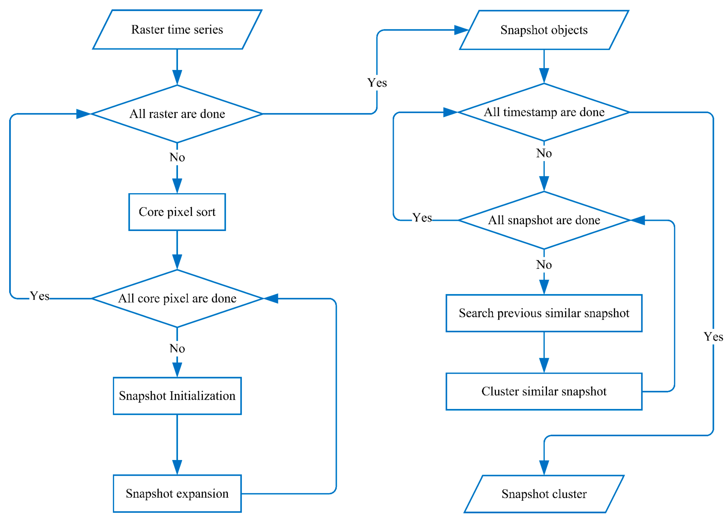
2.2.1. Snapshot Object Extraction

The goal of snapshot object extraction is to cluster spatially adjacent pixels with similar attributes raster by raster and to extract the area covered by such pixels as snapshot objects. The snapshot object’s extraction relies on spatial density clustering utilizing density threshold parameter K and attribute threshold parameter Kth. The steps of snapshot object extraction are summarized in Algorithm 1.

Algorithm 1. Snapshot Object Extraction.

Step1: Scan all pixels and collect core pixels into a list L. Step2: Sort core pixels in list L in descending order based on the distance between pixel attribute and global attribute averages. Step3: Select an unprocessed core pixel from L to initialize a new cluster and add the pixel to an empty queue Q of the cluster. Step4: Pop a core pixel from Q, expand the cluster by incorporating reachable, non-isolated, and unprocessed pixels in spatial neighborhood of the core pixel, and add the new pixels to Q that are also core pixels. Step5: If Q is not empty, repeat step 4 to expand the cluster. Otherwise, jump to step 3 until all core pixels in L have been processed.

In step 2, the goal of sorting is to start clustering from the core pixel with the greatest attribute distance from the precipitation anomaly background, which is approximated by the average attribute of the pixels of all rasters. In step 4, a pixel within the spatial neighborhood of the core pixel is assigned to the core pixel’s cluster if it meets the following three conditions: (1) it has not been clustered; (2) it is reachable from the core pixel’s cluster; (3) it is not an isolated pixel. The reason for excluding isolated pixels is to avoid assigning noise to the cluster edges and merging two clusters without spatial connectivity into a single cluster.

2.2.2. Snapshot Object Clustering

After performing the extraction of snapshot objects of a single raster representing the status at each timestamp, we obtain all independent snapshot objects in the time series. Based on the degree of overlap and attribute distance, snapshot objects with evolutionary relationships at adjacent timestamps are grouped into a spatiotemporal cluster. Each spatiotemporal cluster must contain at least two snapshot objects. The lower bound of attribute similarity is established using the attribute threshold Kth, previously employed in snapshot object extraction, while an overlap threshold θ is introduced to set the lower bound of spatial similarity, as illustrated in Equation (2). If the judgment conditions are met, the two snapshot objects at adjacent timestamps are assigned to the same spatiotemporal cluster.

$$\left|c_i{.att-c}_{i+1}.att\right|\le Kth \mathrm{AND} \left(\frac{\left|c_i\cap c_{i+1}\right|}{\left|c_i\right|}\ge \theta \mathrm{OR} \frac{\left|c_i\cap c_{i+1}\right|}{\left|c_{i+1}\right|}\ge \theta \right)$$

(2)

In the formula, c_i and c_i+1 refer to the snapshot objects at time i and time i + 1, respectively; c_i.att is the average attribute of all pixels in c_i; |c_i| is the number of pixels in c_i; |c_i∩c_i+1|represents the overlapped areas of c_i and c_i+1; and θ is the overlap threshold parameter, whose value range is 0 < θ < 1.

The overlap area between c_i and c_i+1 is calculated to measure spatial similarity. If the proportion of the overlap area in c_i or c_i+1 is no less than θ, c_i and c_i+1 are considered spatially similar. On the other hand, they are considered attribute similar if the attribute distance between them does not exceed the threshold Kth. Unlike snapshot object extraction, when determining whether a new snapshot object can be assigned to a spatiotemporal cluster, the new object is compared to the overlapping snapshot objects of the cluster at an adjacent timestamp instead of the whole cluster. The reason for doing this is that snapshot objects with larger time intervals exhibit weaker relevance in attribute changes and spatial distribution. The pseudocode of spatiotemporal clustering is shown in Algorithm2.

Algorithm 2. Snapshot Object Clustering.

For t in all timestamps         For o in t.Snapshot_Objects              Prev = similar snapshot objects of o at t−1 timestamp              If not the elements of Prev all belong to the same cluster Then                    Merge different clusters of elements to single cluster              Assign o to the cluster of Prev.

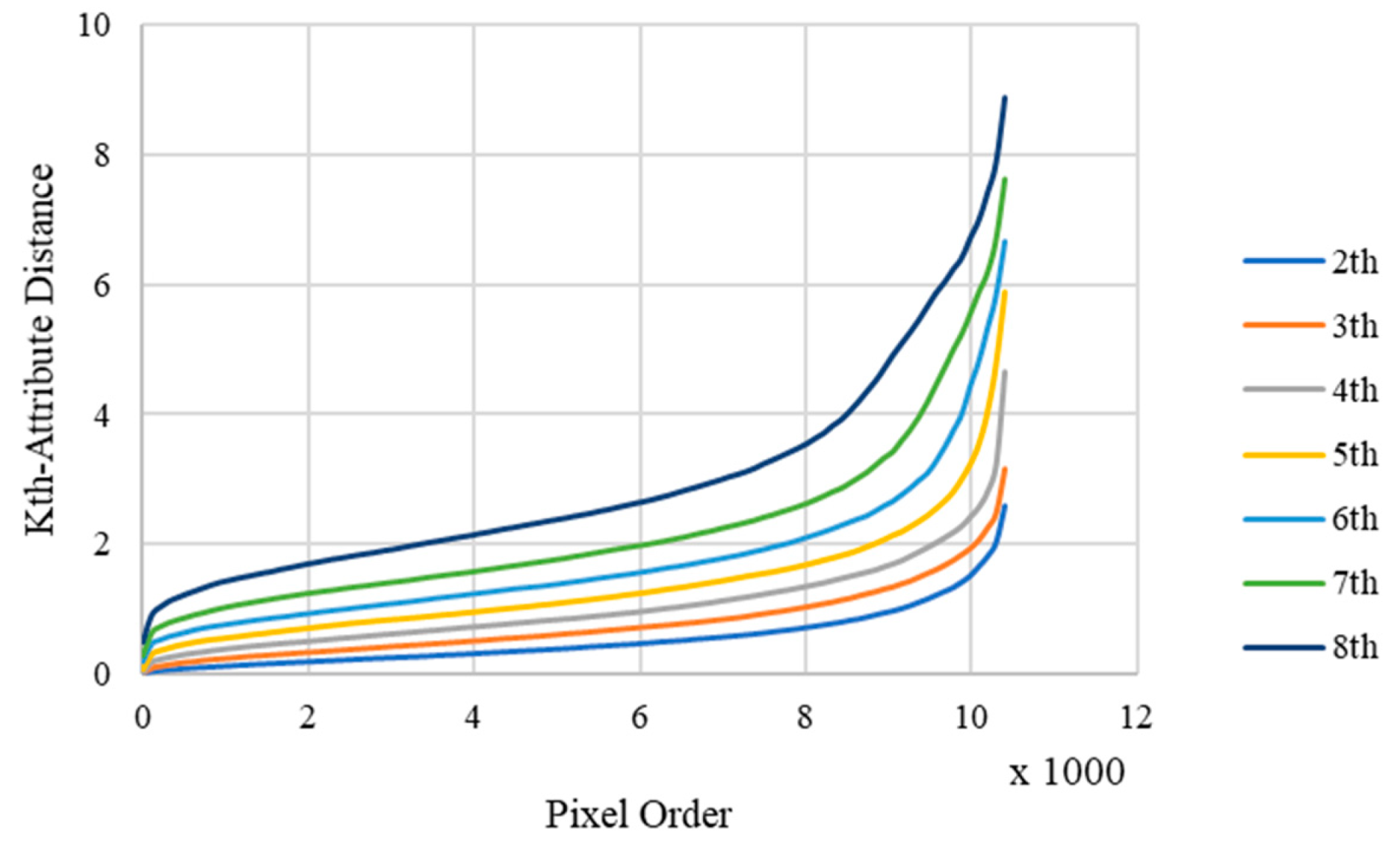
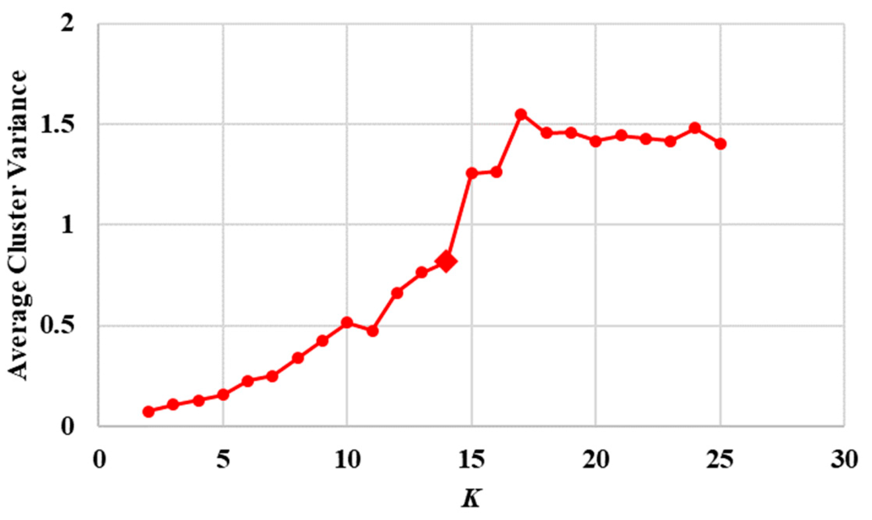
2.2.3. Parameter Setting

The setting of parameter θ requires a rough assessment of the moving speed of precipitation anomaly variations. Generally, θ can be set to 0.5 for precipitation anomaly variations without apparent movement, while a lower value, such as 0.25, should be considered for precipitation anomaly variations with apparent movement.

The parameter Kth is determined by the statistics of the attribute distance between pixels and their Kth spatial neighbors (called Kth-attribute distance). For each K value between 2 and 8, the parameter Kth is computed as follows. First, calculate the Kth-attribute distance of all pixels in the dataset. Subsequently, sort them and draw the change curve in ascending order. Finally, identify the inflection point of the change curve, and set parameter Kth equal to the Kth-attribute distance of this point.

Clustering is performed with different parameter combinations of K and corresponding Kth. The average variance of all clusters in the clustering results is calculated to draw a graph with K as the horizontal axis and average cluster variance as the vertical axis. The final result of the OSCAR is the clustering results of the inflection point in the graph. When computing average cluster variance, the background of the precipitation anomalies is incorporated as a cluster, since average cluster variance without the background cannot reflect the real clustering results. For example, assuming that the variances of all clusters are equal, two parameter combinations resulting in different cluster amounts may have equal average cluster variance. Hence, the variance in the background needs to be considered to ensure that the average cluster variance is comprehensive and accurate.

2.2.4. Complexity

Assuming that there is only one raster at each timestamp, let t represent the number of timestamps and n represent the number of pixels in each raster. The OSCAR comprises two stages: the first stage involves the extraction of snapshot objects, while the second stage focuses on the spatiotemporal clustering of snapshot objects.

The extraction of snapshot objects requires collecting core pixels by traversing and checking all pixels in a raster, resulting in O(n) time complexity. These collected core pixels are then sorted with an average time complexity of O(n log n). Subsequently, the spatial clustering process begins from these core pixels to extract snapshot objects. Considering that all pixels are clustered only once, the time complexity of the clustering process is O(n). To summarize, the time complexity of the snapshot object extraction from one raster is O(n log n). Since the snapshot object extraction is applied to t raster, the total time complexity of snapshot object extraction is O(t n log n).

Spatiotemporal clustering of snapshot objects requires traversing t timestamps chronologically. For each timestamp, previous snapshot objects that are similar to current snapshot objects are searched. Assuming that m_t represents the number of snapshot objects at timestamp t, m_t objects are traversed to search similar snapshot objects among m_t−1 objects. Consequently, the time complexity of searching for similar snapshot objects is O(m_t m_t−1). Although the number of snapshot objects is significantly lower than the number of pixels in a raster, larger rasters contain typically more snapshot objects. Therefore, it is assumed that the number of snapshot objects m is directly proportional to the number of pixels n in a raster. The time complexity of searching for similar snapshot objects is O(n²). As each timestamp is traversed, the time complexity of spatiotemporal clustering is O(t n²).

In conclusion, the time complexity of the OSCAR is O(t n²), meaning it is proportional to the number of timestamps and the square of the number of pixels in each raster.

3. Results

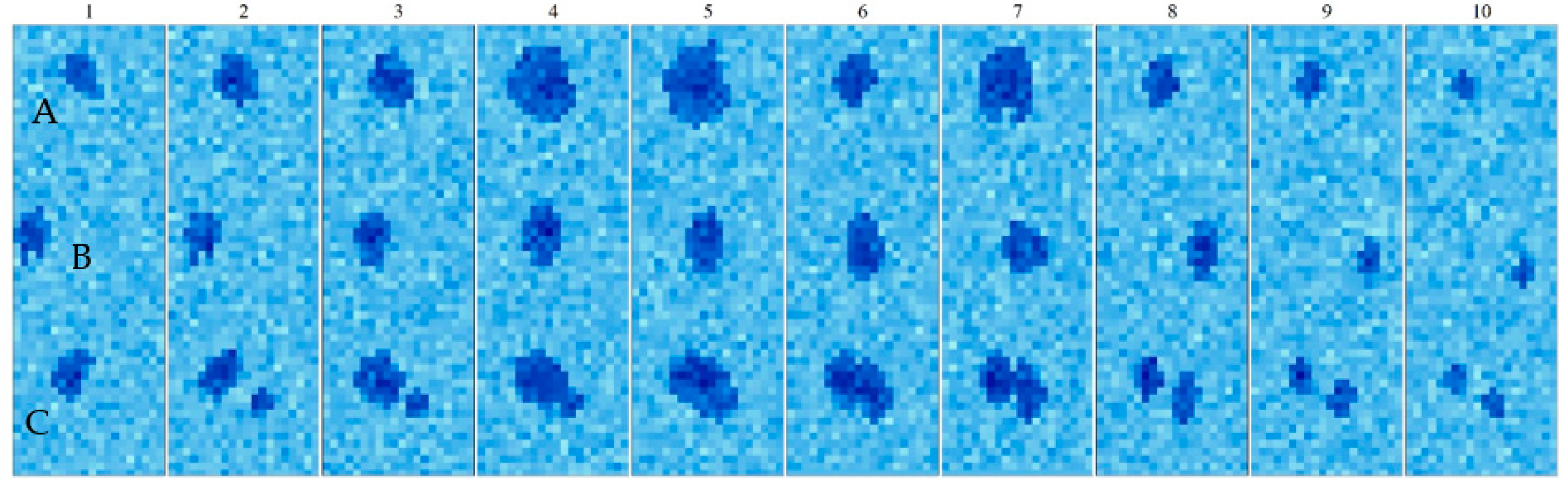
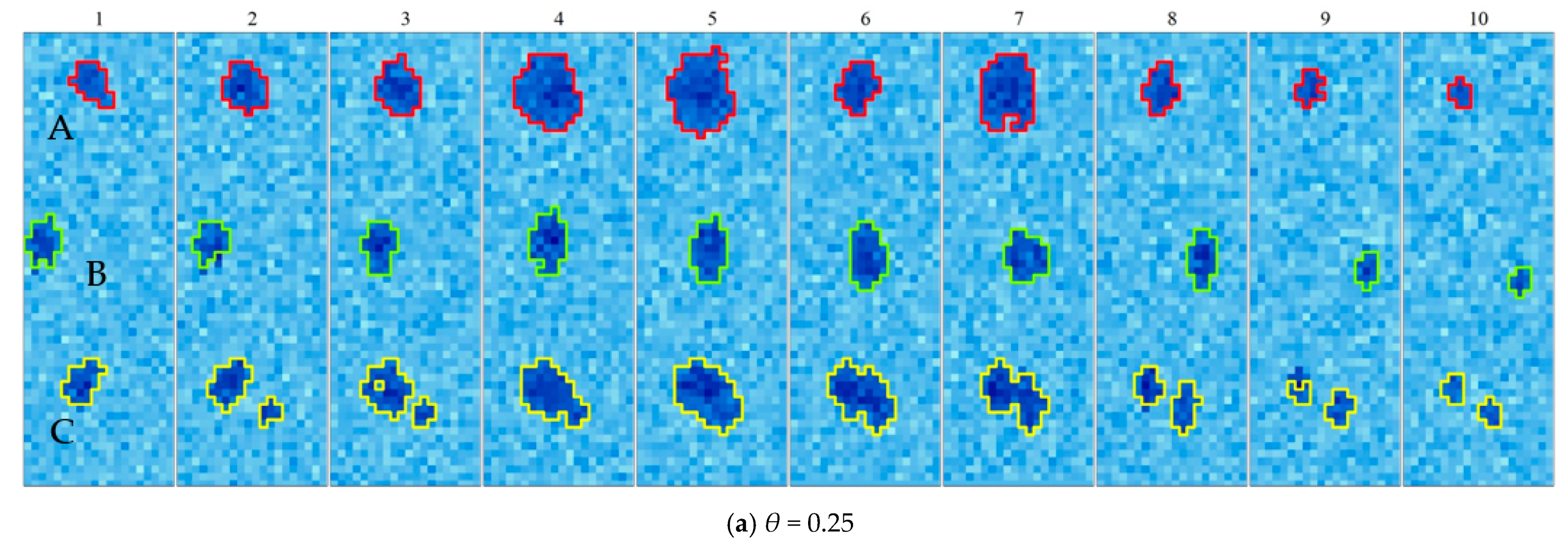
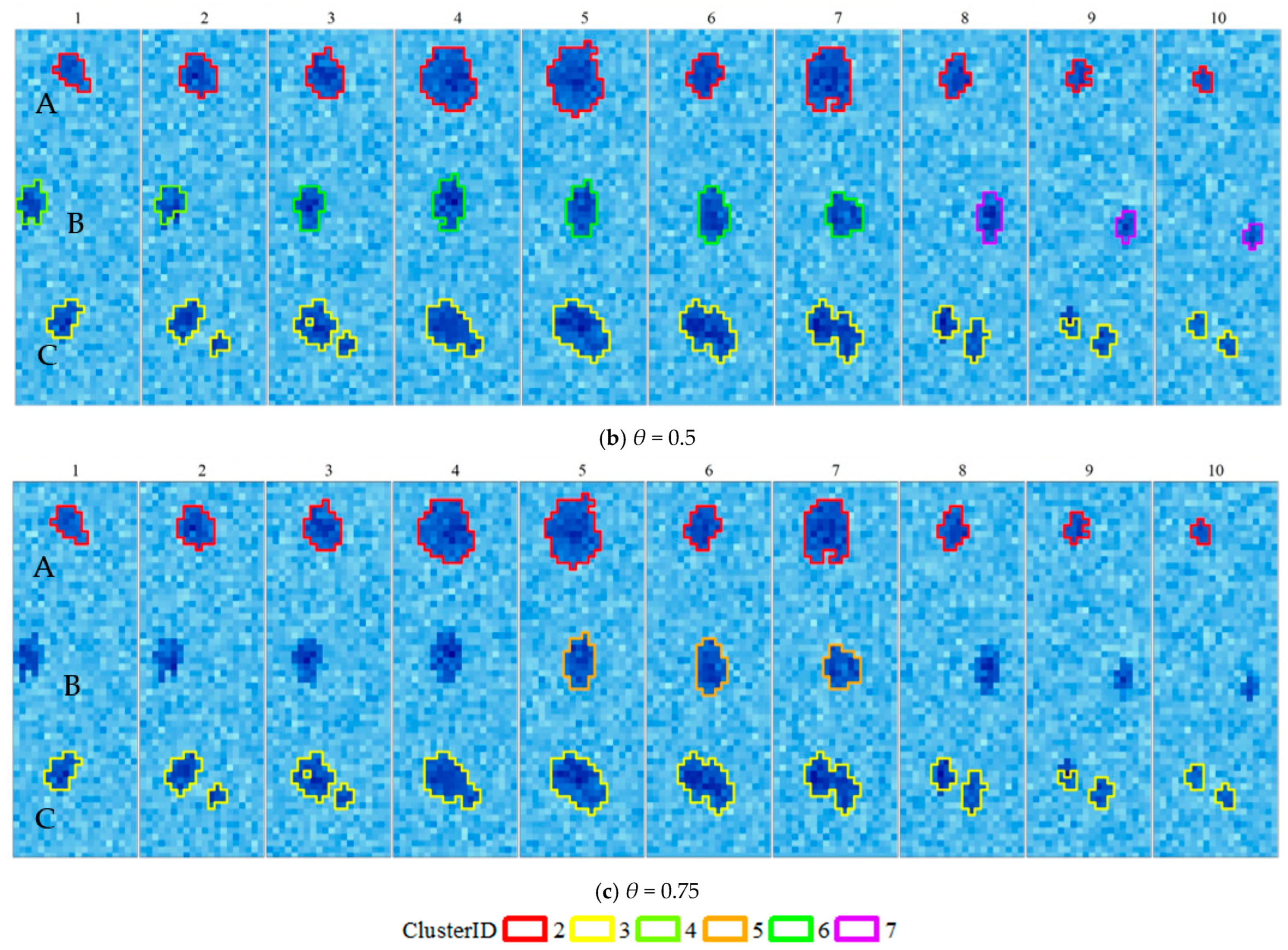
3.1. Experiments on Simulated Dataset

Through statistics on the simulated dataset, all pixels were sorted based on their Kth-attribute distance. The curves of the pixels are plotted in ascending order in Figure 3. The various K and corresponding Kth were obtained based on the inflection points of those curves, which are presented in

Table 1. Parameter combination.

K	Kth
2	2.04
3	2.48
4	2.81
5	3.01
6	3.09
7	3.95
8	4.52

. The parameter θ in the range from 0 to 1 was set to 0.25, 0.5, and 0.75. The parameter combinations of θ, K, and Kth were inputted to the OSCAR to cluster the simulated dataset. The average cluster variance in the different parameter combinations of θ, K, and Kth is depicted in Figure 4. The clustering result when K was 6 was taken as the final result of the OSCAR.

The final result of the OSCAR with distinct θ values is illustrated in Figure 5. The evolution processes of development and disappearance (process A) and merging and splitting (process C) were accurately identified, regardless of which value of θ was used. Nevertheless, for the moving process (process B), the results differed substantially based on θ values. When θ is 0.25, process B at each timestamp could be effectively recognized. Conversely, when θ was set to 0.5, process B was insufficiently identified, resulting in discontinuous spatiotemporal clusters. The speed of process B around timestamp 3 and 7 was fast, causing lower degrees of overlap between snapshot objects at successive timestamps. Therefore, the cluster expansion of process B was interrupted in time dimension and divided into three spatiotemporal clusters: clusters 4, 6, and 7. With θ at 0.75, the process B was only detected when movement was comparatively slow (during timestamp 5 to 7), which was worse than the result when θ was set as 0.5.

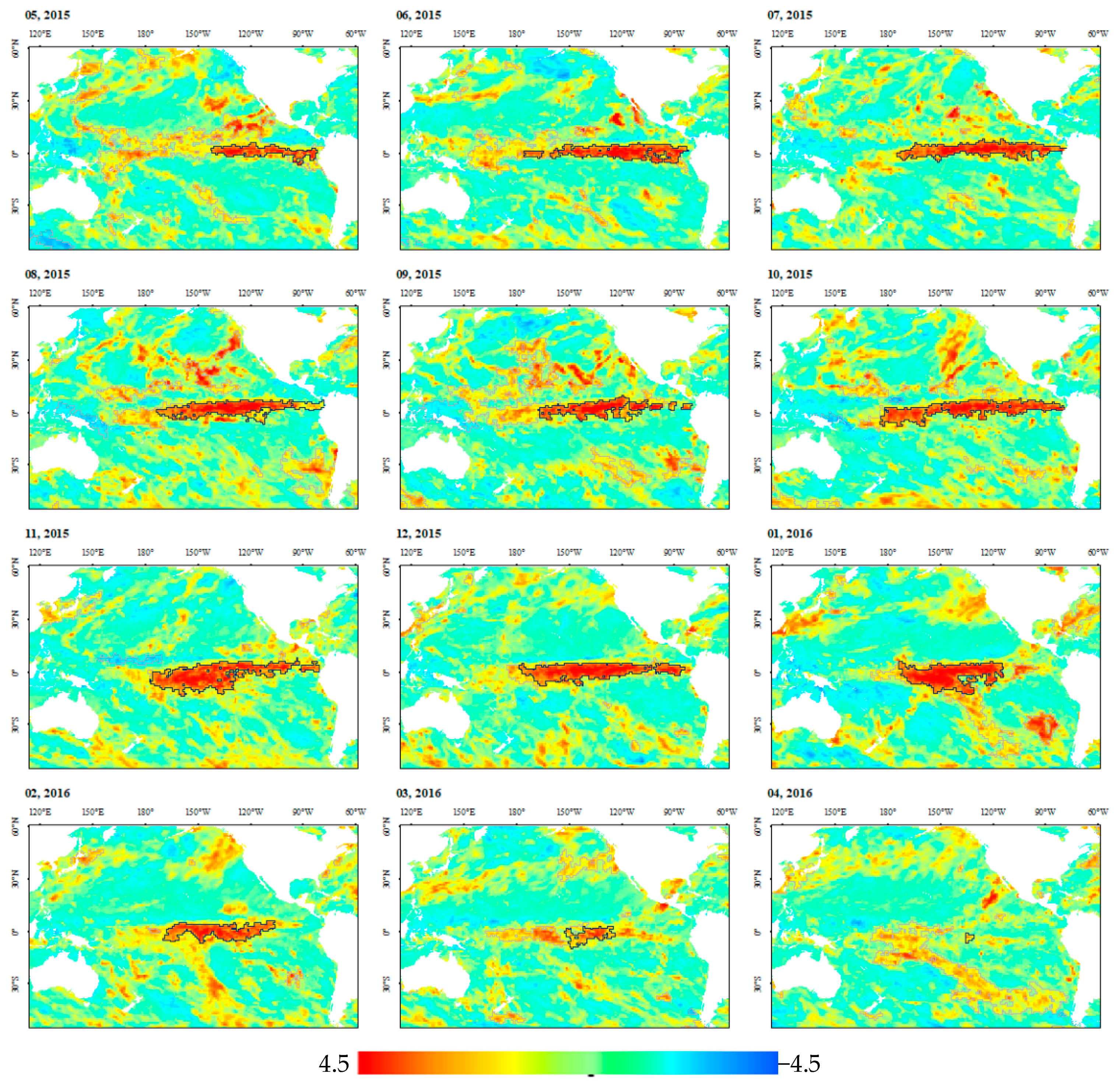
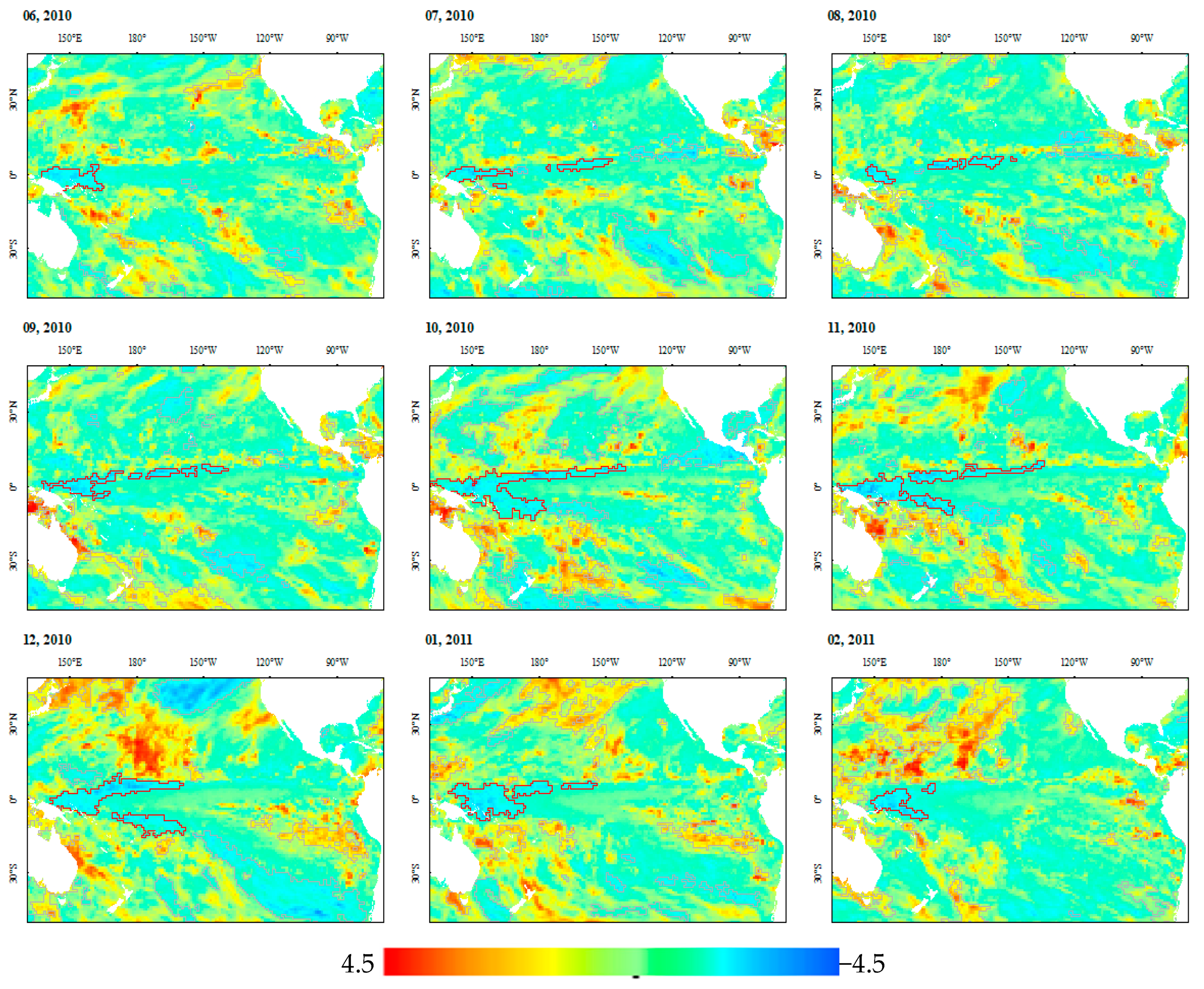
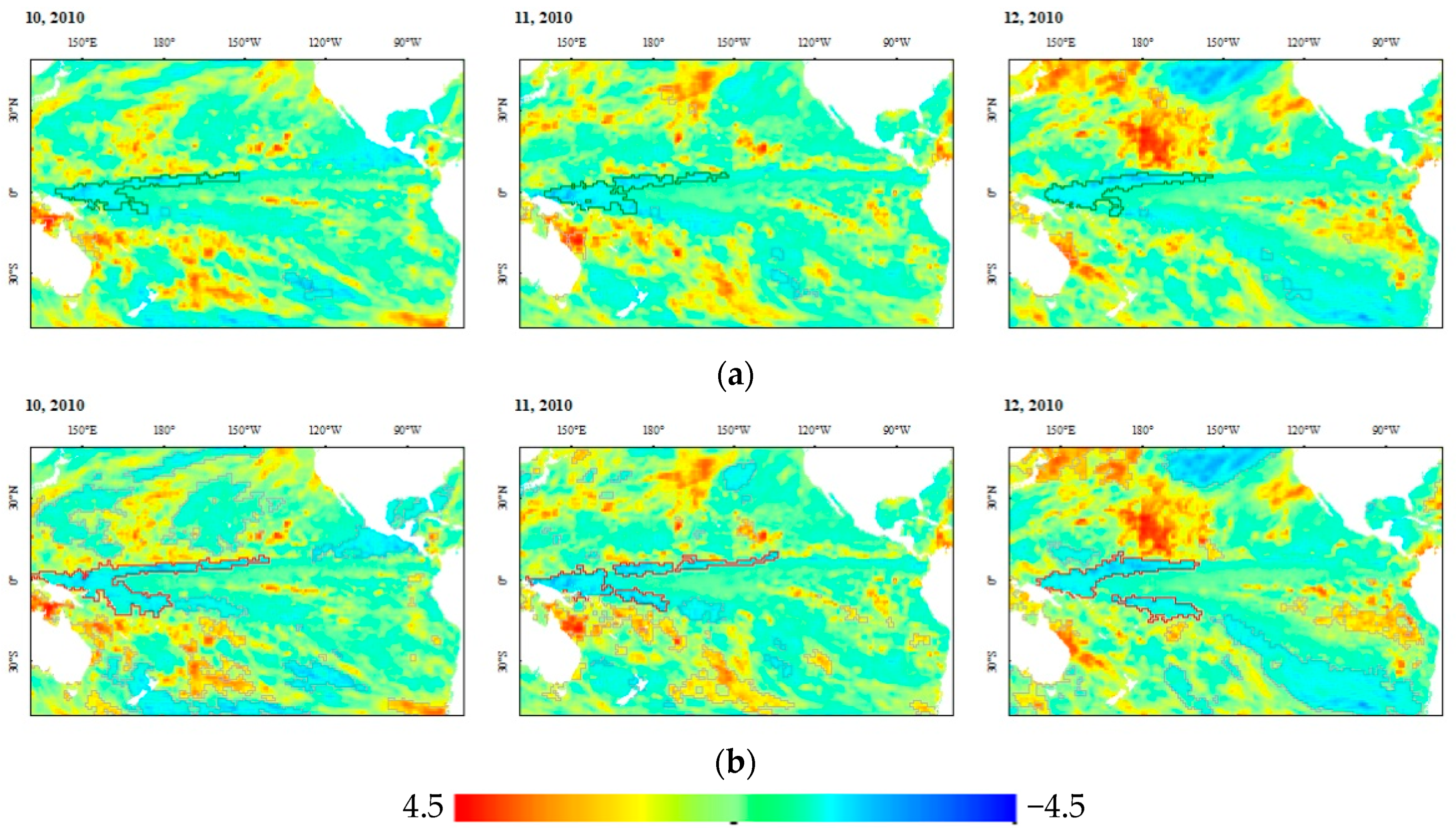
3.2. Case Study of Precipitation Anomalies over the Pacific Ocean

The tropical Pacific region features two prominent precipitation zones, the Pacific intertropical convergence zone (ITCZ) and the South Pacific convergence zone (SPCZ), both of which exhibit associations with the ENSO. During the transition from La Niña to El Niño, the western and central Pacific ITCZ shifts southward by approximately 2° and by nearly 5° during strong El Niño events [33]. A recent study suggested that in the warmer climate of the mid-Pliocene, the ENSO was suppressed by off-equatorial processes initiated by the northward migration of the Pacific ITCZ [34]. The impact of the ENSO on the SPCZ is primarily characterized by the spatial repositioning of the main diagonal axis of precipitation in the SPCZ: under El Niño conditions, the SPCZ diagonal relocates northeastward toward the anomalously warm central and eastern Pacific, while in La Niña conditions, the primary SPCZ diagonal shifts southwestward [35].

The OSCAR was applied to tropical Pacific precipitation anomalies from 2015 to 2016, setting the parameter θ to 0.5, K to 6, and Kth to 1.41. Figure 6 illustrates the spatiotemporal clustering results during the El Niño event, with polygons outlined in dark blue representing typical spatiotemporal clusters and polygons outlined in light gray signifying other clusters.

In May 2015, a spatiotemporal cluster with significantly stronger positive precipitation anomalies than the surrounding areas first emerged in the eastern tropical Pacific, extending westward to the central tropical Pacific. From May to October 2015, the cluster persistently and gradually expanded westward. Between November 2015 and January 2016, the cluster ceased its westward expansion, instead displaying a southward expansion trend in the central tropical Pacific. Concurrently, the positive precipitation anomalies over the eastern tropical Pacific began to weaken, ultimately returning to normal levels by February 2016. Starting from February 2016, the spatiotemporal cluster’s area notably diminished, accompanied by a significant decrease in its anomaly intensity. Eventually, the spatiotemporal cluster ceased in the central tropical Pacific in April 2016.

Figure 7 presents the clustering result of the OSCAR during the La Niña event between 2010 and 2011 when setting θ to 0.5, K to 3, and Kth to 1.03. The negative precipitation anomaly originated in the western tropical Pacific near the coast and expanded progressively eastward and southward. Throughout the La Niña event, the western tropical Pacific persistently maintained a robust negative precipitation anomaly. Conversely, the precipitation anomalies of the central tropical Pacific experienced considerable fluctuations in both spatial coverage and intensity. From June 2010 to September 2010, the cluster extended eastward into the central tropical Pacific. After September 2010, the expansion of the cluster in an easterly direction stalled and began to spread southwards instead. From December 2010 onwards, the spatial extent of the cluster shrunk in the central tropical Pacific until it disappeared completely in February 2011.

4. Discussion

This paper quantitatively evaluated the differences between the OSCAR and the DcSTCA based on the experimental results of the simulated dataset and qualitatively compared the OSCAR and the DcSTCA based on the clustering results of the remote sensing products. In addition, we discussed the relationship between the OSCAR cluster of precipitation anomalies and the ENSO event.

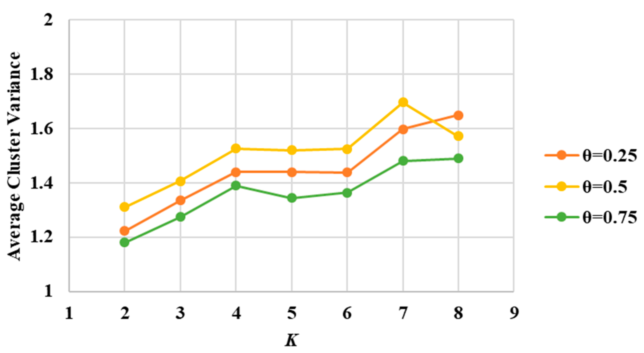
4.1. OSCAR Parameters Setting

As depicted in Figure 3, the predominant feature of the Kth curves is their gradual alteration, with the exception of the tails. This implies that the majority of adjacent pixels in the pixel neighborhood possess minor and analogous attribute distances. Nevertheless, the Kth curves exhibit a sharp incline in the tail, signifying a limited number of anomalous adjacent pixels with extensive and divergent attribute distances, likely attributed to noise. This is why the turning point of the curve serves as the upper threshold for attribute distance.

The overlap threshold parameter θ represents the minimum spatial overlap of the evolution snapshots at adjacent moments. For evolutionary processes that do not move very fast, the value of θ has little effect on the clustering results, e.g., processes A and C in Figure 5. For evolutionary processes that move faster, a too large value of θ may result in incomplete identification of the evolutionary processes, e.g., fast-moving process B in Figure 5. For rapidly moving evolutionary processes, an increase in speed corresponds to diminishing overlapping area of snapshot objects at adjacent timestamps. Therefore, it is necessary to set a low θ value for a fast-moving evolutionary process. The higher movement speed, the lower the assigned value of parameter θ should be. Although there is generally more than one evolutionary process in a remote sensing product dataset, it is sufficient to set the parameter θ according to the fastest moving evolutionary process, since evolutionary processes that can be identified at high θ values can also be identified at low θ values.

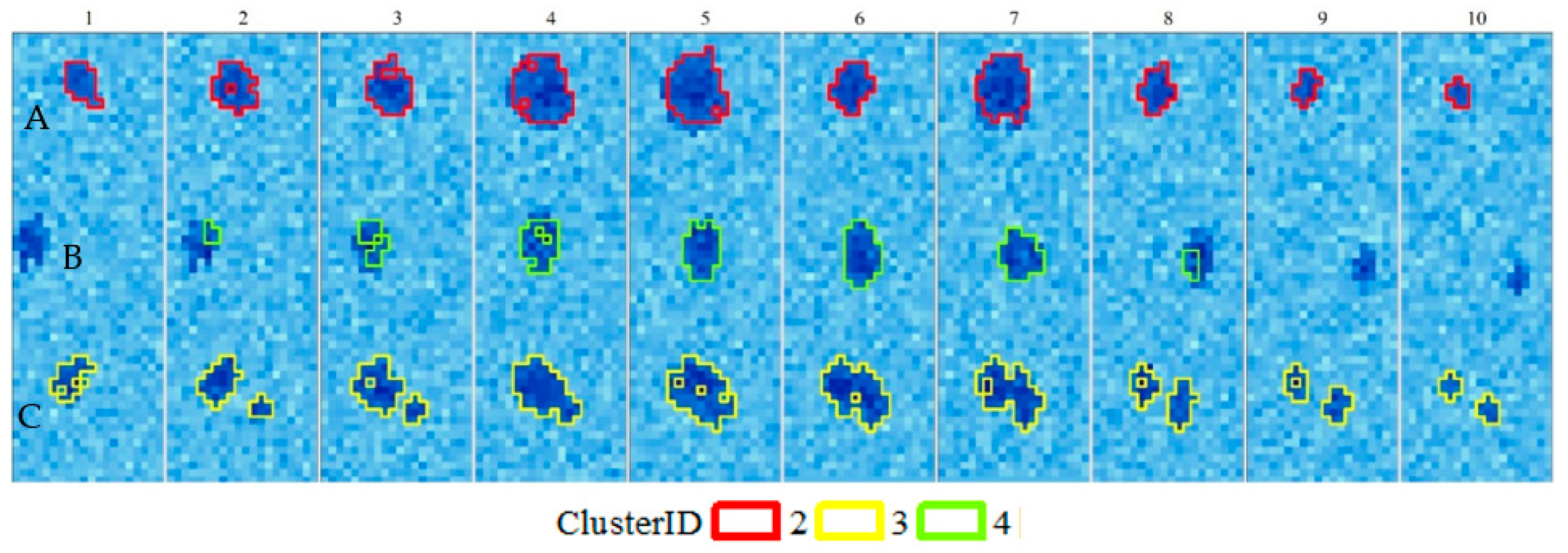
4.2. Quantitative Comparison between OSCAR and DcSTCA

The number threshold and attribute threshold of the DcSTCA were set according to K, while the time interval threshold was fixed at 1. The average cluster variance derived from different parameters is shown in Figure 8. The final result of the DcSTCA was the cluster result when K was 14, as the inflection point of the average cluster variance was where K was 14.

The clusters of the DcSTCA are shown in Figure 9. The time interval threshold, attribute threshold, and number threshold were 1, 0.81, and 14, respectively. The DcSTCA could basically identify the snapshots of processes A and C at various timestamps. For process C, there were many unreasonable holes in cluster 3, especially between timestamp 5 and 9. For process A, some edge pixels were missed at timestamps 4, 5, and 7. Their common feature was that same pixels do not show anomalies at the previous and next timestamps, meaning the anomaly duration does not exceed three timestamps. The DcSTCA’s clustering results for process B were significantly worse, as it could only identify the anomalies that lasted three timestamps.

The inability of the DcSTCA to effectively identify processes A and B stems from its core pixel definition. The DcSTCA requires the core pixel attributes of previous and subsequent timestamps to resemble the current pixel attribute. Consequently, the cluster expansion-based core pixels may miss edge pixels, particularly in areas experiencing rapid changes. In contrast to the DcSTCA, the OSCAR does not consider preceding and following timestamps during the extraction of snapshot objects but takes them into account during the clustering of these objects. As a result, the OSCAR avoids omitting edge pixels when precipitation anomalies change rapidly, ensuring the integrity of snapshot objects.

The Adjusted Rand Index (ARI) and Normalized Mutual Information (NMI) indices of the OSCAR and the DcSTCA are presented in

Table 2. Clustering evaluation index.

Index/Algorithm	DcSTCA	OSCAR	OSCAR (θ = 0.25)	OSCAR (θ = 0.5)	OSCAR (θ = 0.75)
ARI	0.88	0.95	0.98	0.98	0.89
NMI	0.81	0.91	0.96	0.94	0.85

. The accuracy of the OSCAR, regardless of the value of θ, was significantly higher than the accuracy of the DcSTCA. Notably, when θ was set to 0.25, the ARI and NMI indices of OSCAR reached 0.98 and 0.96, respectively. Even in the worst case, with θ at 0.75, OSCAR’s accuracy still surpassed that of the DcSTCA. The average ARI and NMI of the OSCAR were 0.95 and 0.91, respectively, markedly outperforming the DcSTCA’s scores of 0.88 and 0.81. In conclusion, the OSCAR showed overall higher effectiveness and precision than the DcSTCA, especially for the evolution processes that change rapidly in spatial distribution.

4.3. Qualitative Comparison between OSCAR and DcSTCA

The DcSTCA was applied to the same dataset, employing a time interval threshold of 2, an attribute threshold of 1.93, and a number threshold of 24, and was compared to the OSCAR, as shown in Figure 10. In the figure, polygons outlined in purple indicate typical tropical Pacific spatiotemporal clusters, while light gray polygons represent other clusters. The figure shows significant discrepancies in thematic attributes for pixels within snapshots. In other words, the thematic attributes are inconsistent within the snapshots. The clustering of the DcSTCA encompassed the weakly anomalous regions at the western and eastern edges but did not encompass the strongly anomalous region at the southern edge, where the precipitation anomaly was more similar to the precipitation anomaly of the whole cluster. As the precipitation anomalies extended southward, the DcSTCA could not recognize the complete extended areas to the south in November 2015 and January 2016, omitting some edge pixels. This is because the extended areas were not anomalous in the previous and next months. In contrast, the pixels within the snapshot objects of the OSCAR results had more consistent precipitation anomalies. Furthermore, the prominent areas on the southern edge of the cluster were accurately identified.

Figure 11 illustrates the clustering result achieved by the DcSTCA with a number threshold of 30 and an attribute threshold of 2.38 compared to the OSCAR. Referring to the literature on the DcSTCA, the time interval parameter was set to 2 based on ENSO events lasting at least five months [29].

The DcSTCA could not entirely identify the southward expanding region of the precipitation anomaly over the eastern tropical Pacific in November and December of 2010. A similar issue also appears in Figure 10, due to the fact that the region expanding to the south was temporary and did not last for more than the time interval threshold. In contrast, the OSCAR avoids this problem by considering the time factor during the clustering of snapshot objects, rather than during the extraction of snapshot objects, where spatial and attribute factors are used instead.

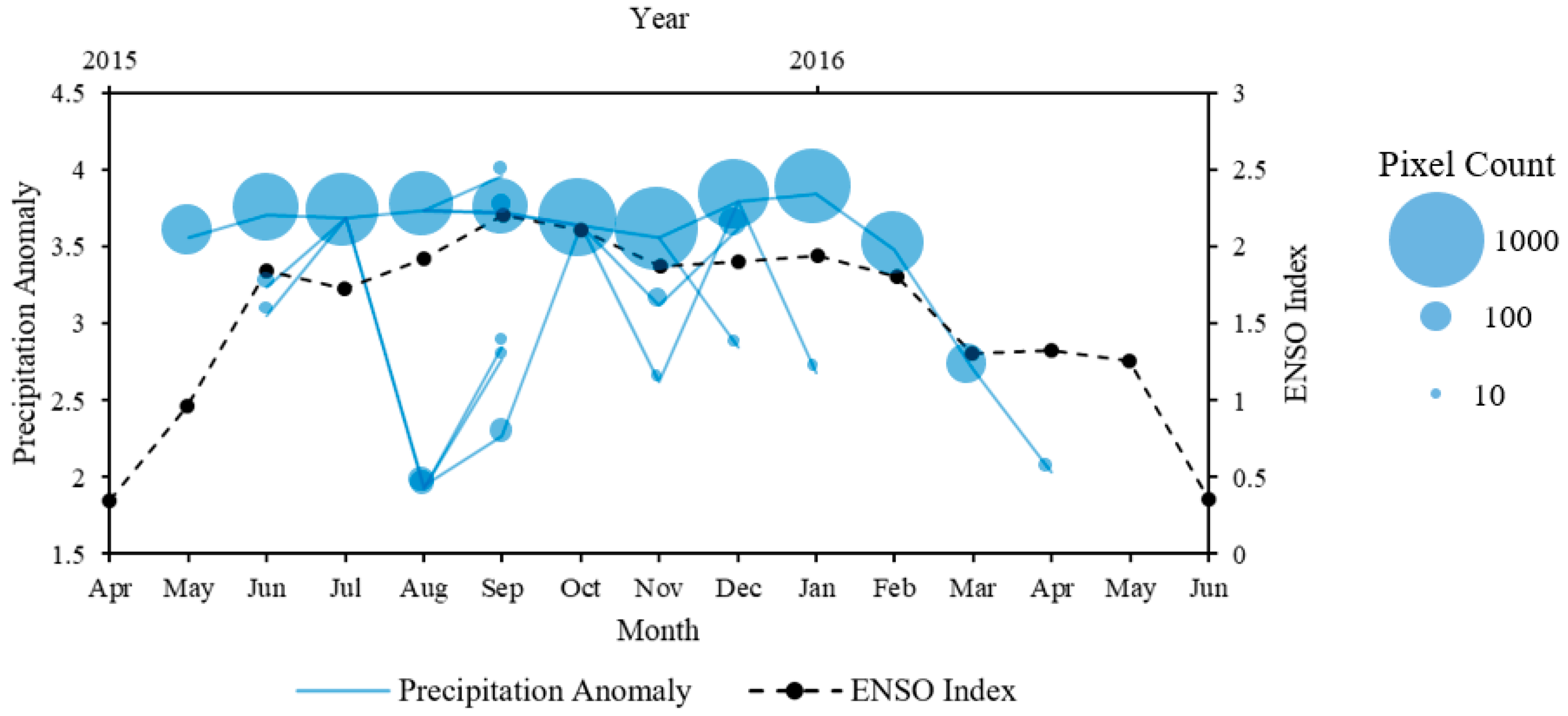
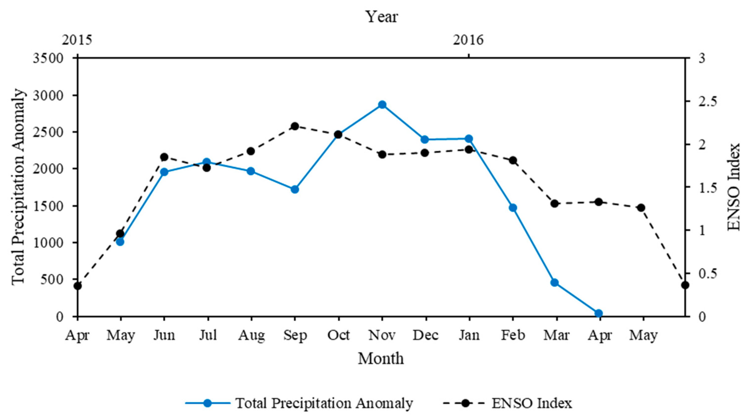
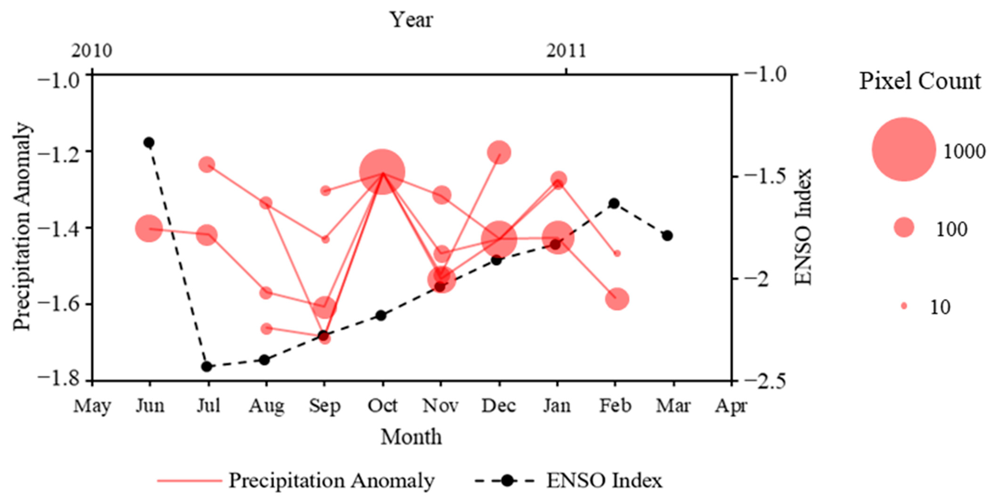
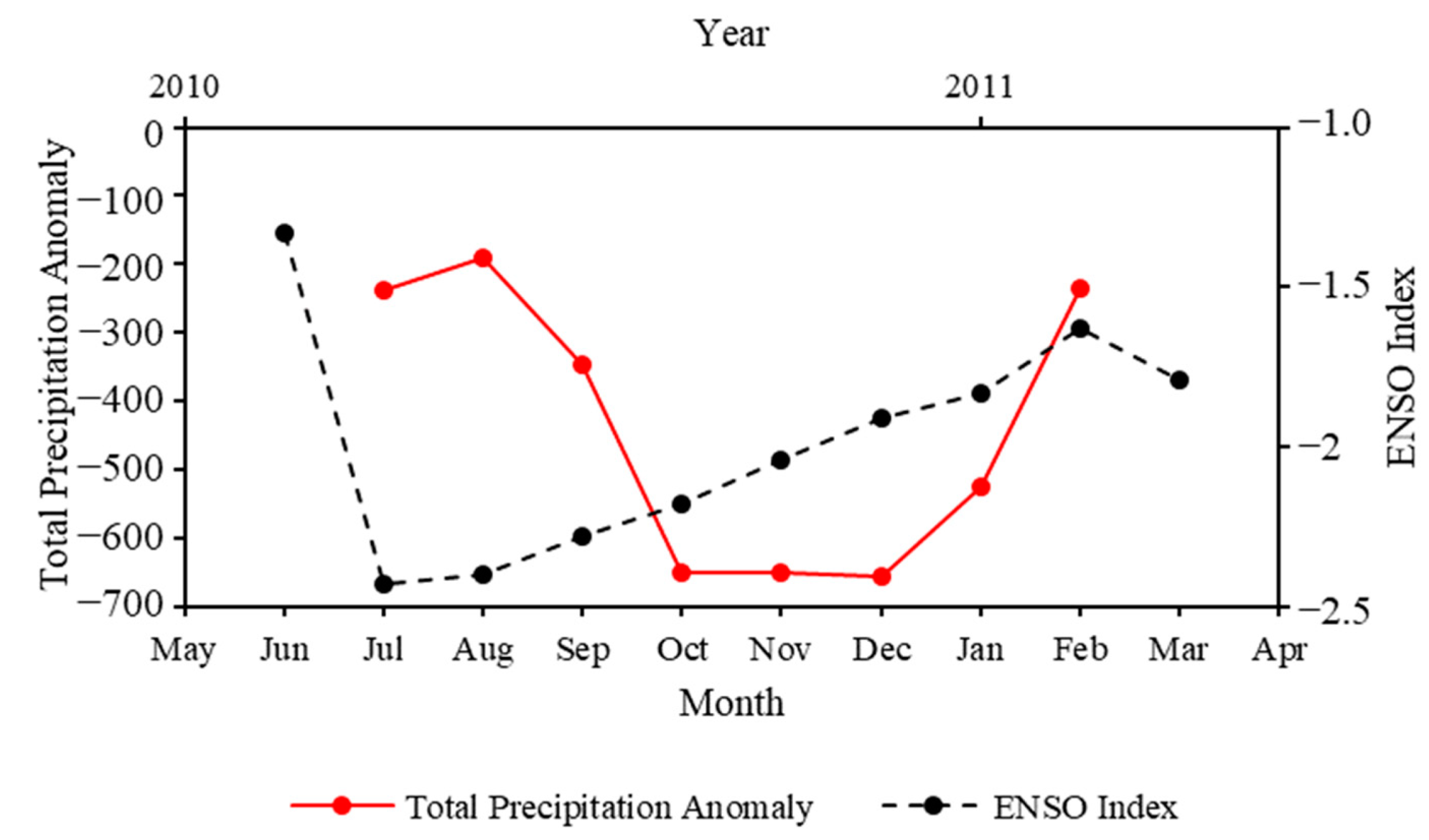
4.4. Relationship between Precipitation Anomalies Clusters and ENSO

The relationship between the ENSO index and the snapshot object of the precipitation anomaly clusters is shown in Figure 12, excluding snapshot objects smaller than 10 pixels. In this figure, the precipitation anomaly of the node center represents the mean precipitation anomaly of the snapshot object, while the node area correlates to the number of pixels with a size of 1° × 1°. The edge between nodes represents the evolutionary relationship between snapshot objects, such as development, merging, and splitting. The cluster began in May 2015, when the ENSO index first exceeded 0.5, marking the start of an El Niño event. The average anomaly of the snapshot object with the largest area tended to change as the ENSO event evolves, particularly from September 2015 to March 2016. As the ENSO index began to decrease in January 2016, the area and anomaly of the cluster experienced an accelerated decline. The duration of the cluster was comparable to that of the El Niño event, which ended in May 2016. In addition, the precipitation anomaly trend of the largest snapshot object was synchronized with the strength variation in the El Niño event.

Figure 13 represents the relationship between the ENSO index and the total precipitation anomaly of the clusters, that is, the sum of the precipitation anomalies of all pixels at a given timestamp. As with the ENSO index, the total precipitation anomaly was at a high level between June 2015 and January 2016. Then, the total precipitation anomaly of the cluster weakened and disappeared before the El Niño event.

Figure 14 illustrates the relationship between the ENSO index and the precipitation anomaly cluster (excluding those smaller than 10 pixels) with the node corresponding to the snapshot object. The change trends in the lowest monthly anomaly of the snapshot objects were roughly synchronized with the development of the La Niña event, with the exception of October 2010, when the snapshot objects temporarily merged into a large object with a slight precipitation anomaly. As the ENSO index dropped rapidly to a minimum value of −2.43 in July 2010, the precipitation anomaly also reached a minimum after a delay of two months. Then, the precipitation anomaly increased with the rising ENSO index after September 2010 and bounced back a month early.

The relationship between the La Niña event and the total precipitation anomaly of the clusters is displayed in Figure 15. The clusters only occurred around the height of the La Niña. The strengthening of the negative precipitation anomaly was delayed compared to the La Niña event. The total precipitation anomaly of the cluster reached its minimum in October 2010, later than the ENSO index, but it rose even faster after staying at a low level from October 2010 to December 2010. The total precipitation anomaly and the La Niña event simultaneously returned to their initial levels in February 2011.

5. Conclusions

Extreme precipitation events influenced by the ENSO serve as a critical pathway by which the ENSO impacts the global climate. Specifically, the precipitation induced by the ENSO in the tropical Pacific has the potential to trigger extreme weather occurrences globally, leading to substantial harm to agriculture, ecosystems, and economic stability. However, existing spatiotemporal clustering algorithms face challenges in effectively identifying rapidly changing variations in sea surface precipitation anomalies. To address this issue, this paper proposes an object-oriented spatiotemporal clustering algorithm using remote sensing products (OSCAR) to identify the evolution of precipitation anomalies.

The OSCAR was validated using simulated datasets and compared with traditional DcSTCA. The results of the experiment show that the OSCAR is more effective in identifying rapidly changing precipitation anomaly variations compared to the DcSTCA. Additionally, the OSCAR exhibits higher accuracy than the DcSTCA, as evidenced by the improvements in the ARI and NMI of the clustering results from 0.88 and 0.81 to 0.95 and 0.91, respectively. This validation study demonstrates the effectiveness of the OSCAR in recognizing spatiotemporal clustering patterns of variations in precipitation anomalies.

The OSCAR was utilized to spatiotemporally cluster ENSO-related precipitation anomalies in the tropical Pacific region. The experimental results indicate that positive anomaly clusters are observed in the central-eastern tropical Pacific during El Niño events, while negative anomaly clusters appear in the western-central tropical Pacific during La Niña events. These findings align with prior research based on static statistical values [4,16,36], demonstrating the efficacy of the OSCAR in detecting the evolution of ENSO-related precipitation anomalies. Moreover, the tropical Pacific precipitation anomalies in the cold and warm ENSO phases intensify with ENSO events. Specifically, positive precipitation anomalies amplify with El Niño events while negative precipitation anomalies strengthen with La Niña events. These insights may offer valuable reference for comprehending the feedback and driving mechanism between tropical Pacific precipitation and ENSO.

In addition to precipitation, marine environmental variables such as sea surface temperature and sea level height exhibit continuous evolution characteristics, reflected in the spatial and temporal continuity of their thematic attributes. In the future, the OSCAR method is anticipated to be employed in the analysis of other marine environmental data to investigate the connection between the ENSO and the evolutionary processes of other marine environment variables.

References

1. Neelin, J.D.; Battisti, D.S.; Hirst, A.C.; Jin, F.-F.; Wakata, Y.; Yamagata, T.; Zebiak, S.E. ENSO theory. J. Geophys. Res. 1998, 103, 14261–14290. [Google Scholar] [CrossRef] [Green Version]
2. McPhaden, M.J.; Zebiak, S.E.; Glantz, M.H. ENSO as an integrating concept in earth science. Science 2006, 314, 1740–1745. [Google Scholar] [CrossRef] [PubMed] [Green Version]
3. Deser, C.; Alexander, M.A.; Xie, S.-P.; Phillips, A.S. Sea Surface Temperature Variability: Patterns and Mechanisms. Annu. Rev. Mar. Sci. 2010, 2, 115–143. [Google Scholar] [CrossRef] [PubMed] [Green Version]
4. Huang, P.; Xie, S.-P. Mechanisms of change in ENSO-induced tropical Pacific rainfall variability in a warming climate. Nat. Geosci. 2015, 8, 922–926. [Google Scholar] [CrossRef]
5. Power, S.; Delage, F.; Chung, C.; Kociuba, G.; Keay, K. Robust twenty-first-century projections of El Niño and related precipitation variability. Nature 2013, 502, 541–545. [Google Scholar] [CrossRef]
6. Cai, W.; Borlace, S.; Lengaigne, M.; van Rensch, P.; Collins, M.; Vecchi, G.; Timmermann, A.; Santoso, A.; McPhaden, M.J.; Wu, L.; et al. Increasing frequency of extreme El Niño events due to greenhouse warming. Nat. Clim. Chang. 2014, 4, 111–116. [Google Scholar] [CrossRef] [Green Version]
7. Alexander, M.A.; Bladé, I.; Newman, M.; Lanzante, J.R.; Lau, N.C.; Scott, J.D. The atmospheric bridge: The influence of ENSO teleconnections on air-sea interaction over the global oceans. J. Clim. 2002, 15, 2205–2231. [Google Scholar] [CrossRef]
8. Yan, Z.; Wu, B.; Li, T.; Collins, M.; Clark, R.; Zhou, T.; Murphy, J.; Tan, G. Eastward shift and extension of ENSO-induced tropical precipitation anomalies under global warming. Sci. Adv. 2020, 6, eaax4177. [Google Scholar] [CrossRef] [Green Version]
9. Yang, Y.; Park, J.; An, S.; Bin, W.; Xiao, L. Mean sea surface temperature changes influence ENSO-related precipitation changes in the mid-latitudes. Nat. Commun. 2021, 12, 1495. [Google Scholar] [CrossRef]
10. Maes, C.; Belamari, S. On the impact of salinity barrier layer on the Pacific ocean mean state and ENSO. SOLA 2011, 7, 97–100. [Google Scholar] [CrossRef] [Green Version]
11. Zhu, J.; Huang, B.; Zhang, R.-H.; Hu, Z.-Z.; Kumar, A.; Balmaseda, M.A.; Marx, L.; Kinter, J.L., III. Salinity anomaly as a trigger for ENSO events. Sci. Rep. 2014, 4, 6821. [Google Scholar] [CrossRef] [Green Version]
12. Zhang, R.-H. A hybrid coupled model for the Pacific ocean-atmosphere system. Part I, description and basic performance. Adv. Atmos. Sci. 2015, 32, 301–318. [Google Scholar] [CrossRef]
13. Kang, X.; Zhang, R.-H.; Wang, G. Effects of different freshwater flux representations in an ocean general circulation model of the tropical Pacific. Sci. Bull. 2017, 62, 345–351. [Google Scholar] [CrossRef]
14. Gao, C.; Zhang, R.-H.; Karnauskas, K.B.; Zhang, L.; Tian, F. Separating freshwater flux effects on ENSO in a hybrid coupled model of the tropical Pacific. Clim. Dyn. 2020, 54, 4605–4626. [Google Scholar] [CrossRef]
15. Zhi, H.; Zhang, R.-H.; Lin, P.; Yu, P.; Zhou, G.; Shi, S. Interannual salinity variability associated with the Central Pacific and Eastern Pacific El Niños in the tropical Pacific. J. Geophys. Res. 2020, 125, e2020JC016090. [Google Scholar] [CrossRef]
16. Zhu, Y.; Zhang, R.-H. A deep learning–based U-Net model for ENSO-related precipitation responses to sea surface temperature anomalies over the tropical Pacific. Atmos. Ocean. Sci. Lett. 2023, 100351. [Google Scholar] [CrossRef]
17. Yang, J.; Gong, P.; Fu, R.; Zhang, M.; Chen, J.; Liang, S.; Xu, B.; Shi, J.; Dickinson, R. The role of satellite remote sensing in climate change studies. Nat. Clim. Chang. 2013, 3, 875–883. [Google Scholar] [CrossRef]
18. Pike, M.; Lintner, B.R. Application of Clustering Algorithms to TRMM Precipitation over the Tropical and South Pacific Ocean. J. Clim. 2020, 33, 5767–5785. [Google Scholar] [CrossRef] [Green Version]
19. Wang, B.; Luo, X.; Liu, J. How Robust is the Asian Precipitation–ENSO Relationship during the Industrial Warming Period (1901–2017)? J. Clim. 2020, 33, 2779–2792. [Google Scholar] [CrossRef]
20. Ma, T.; Chen, W.; Chen, S.; Garfinkel, C.I.; Ding, S.; Song, L.; Li, Z.; Tang, Y.; Huangfu, J.; Gong, H.; et al. Different ENSO Teleconnections over East Asia in Early and Late Winter: Role of Precipitation Anomalies in the Tropical Indian Ocean and Far Western Pacific. J. Clim. 2022, 35, 7919–7935. [Google Scholar] [CrossRef]
21. Dixon, M.; Wiener, G.; Technology, O. TITAN: Thunderstorm Identification, Tracking, Analysis, and Nowcasting—A Radar-based Methodology. J. Atmos. Ocean. Technol. 1993, 10, 785–797. [Google Scholar] [CrossRef]
22. Lakshmanan, V.; Hondl, K.; Rabin, R. An Efficient, General-Purpose Technique for Identifying Storm Cells in Geospatial Images. J. Atmos. Ocean. Technol. 2009, 26, 523–537. [Google Scholar] [CrossRef]
23. Muñoz, C.; Wang, L.-P.; Willems, P. Enhanced object-based tracking algorithm for convective rain storms and cells. Atmos. Res. 2018, 201, 144–158. [Google Scholar] [CrossRef]
24. Han, L.; Fu, S.; Zhao, L.; Zheng, Y.; Wang, H.; Lin, Y. 3D Convective Storm Identification, Tracking, and Forecasting—An Enhanced TITAN Algorithm. J. Atmos. Ocean. Technol. 2009, 26, 719–732. [Google Scholar] [CrossRef]
25. Liu, W.B.; Li, X.G.; Rahn, D.A. Storm event representation and analysis based on a directed spatiotemporal graph model. Int. J. Geogr. Inf. Sci. 2016, 30, 948–969. [Google Scholar] [CrossRef]
26. Lu, E.; Zou, X.; Zhao, C.; Zhao, W.; Ye, D.; Zhang, Q. Temporal–Spatial Monitoring of an Extreme Precipitation Event, Determining Simultaneously the Time Period It Lasts and the Geographic Region It Affects. J. Clim. 2017, 30, 6123–6132. [Google Scholar] [CrossRef]
27. Hou, J.; Wang, P. Tracking via Tree Structure Representation of Radar Data. J. Atmos. Ocean. Technol. 2017, 34, 729–747. [Google Scholar] [CrossRef]
28. Xue, C.; Liu, J.; Yang, G.; Wu, C. A Process-Oriented Method for Tracking Rainstorms with a Time-Series of Raster Datasets. Appl. Sci. 2019, 9, 2468. [Google Scholar] [CrossRef] [Green Version]
29. Liu, J.; Xue, C.; He, Y.; Dong, Q.; Kong, F.; Hong, Y. Dual-Constraint Spatiotemporal Clustering Approach for Exploring Marine Anomaly Patterns Using Remote Sensing Products. IEEE J. Sel. Top. Appl. Earth Obs. Remote Sens. 2018, 11, 3963–3976. [Google Scholar] [CrossRef]
30. Li, L.; Xu, Y.; Xue, C.; Fu, Y.; Zhang, Y. A Process-Oriented Approach to Identify Evolutions of Sea Surface Temperature Anomalies with a Time-Series of a Raster Dataset. ISPRS Int. J. Geo-Inf. 2021, 10, 500. [Google Scholar] [CrossRef]
31. Xue, C.; Xu, Y.; He, Y. A global process-oriented sea surface temperature anomaly dataset retrieved from remote sensing products. Big Earth Data 2022, 6, 179–195. [Google Scholar] [CrossRef]
32. Wolter, K.; Timlin, M.S. Measuring the strength of ENSO events-how does 1997/98 rank? Weather 1998, 53, 315–324. [Google Scholar] [CrossRef]
33. Schneider, T.; Bischoff, T.; Haug, G.H. Migrations and dynamics of the intertropical convergence zone. Nature 2014, 513, 45–53. [Google Scholar] [CrossRef]
34. Pontes, G.M.; Taschetto, A.S.; Sen Gupta, A.; Santoso, A.; Wainer, I.; Haywood, A.M.; Chan, W.-L.; Abe-Ouchi, A.; Stepanek, C.; Lohmann, G.; et al. Mid-Pliocene El Niño/Southern Oscillation suppressed by Pacific intertropical convergence zone shift. Nat. Geosci. 2022, 15, 726–734. [Google Scholar] [CrossRef]
35. Folland, C.K.; Renwick, J.A.; Salinger, M.J.; Mullan, A.B. Relative influences of the Interdecadal Pacific Oscillation and ENSO on the South Pacific Convergence Zone. Geophys. Res. Lett. 2002, 29, 21-1–21-4. [Google Scholar] [CrossRef]
36. Zhang, R.-H.; Busalacchi, A.J. Freshwater flux (FWF)-induced oceanic feedback in a hybrid coupled model of the tropical Pacific. J. Clim. 2009, 22, 853–879. [Google Scholar] [CrossRef]
Figure 1. Simulated raster dataset. The numbers 1–10 and the alphabet ABC are a unique identifier of the timestamp and the evolutionary process, respectively.
Remotesensing 15 02902 g001
Figure 2. Workflow of the OSCAR.
Remotesensing 15 02902 g002
Figure 3. Curves of Kth-attribute distance.
Remotesensing 15 02902 g003
Figure 4. The average attributes variance within clusters.
Remotesensing 15 02902 g004
Figure 5. Clustering results of the OSCAR with distinct θ. The numbers 1–10 and the alphabet ABC are a unique identifier of the timestamp and the evolutionary process, respectively.
Remotesensing 15 02902 g005aRemotesensing 15 02902 g005b
Figure 6. The OSCAR results during the El Niño event.
Remotesensing 15 02902 g006
Figure 7. The OSCAR results during the La Niña event.
Remotesensing 15 02902 g007
Figure 8. The average variance of the attributes within clusters.
Remotesensing 15 02902 g008
Figure 9. Clustering results of the DcSTCA. The numbers 1–10 and the alphabet ABC are a unique identifier of the timestamp and the evolutionary process, respectively.
Remotesensing 15 02902 g009
Figure 10. Comparison of the results of the DcSTCA (a) and the OSCAR (b) during El Niño.
Remotesensing 15 02902 g010
Figure 11. Comparison of the results of the DcSTCA (a) and the OSCAR (b) during La Niña.
Remotesensing 15 02902 g011
Figure 12. The relationship between ENSO index and the precipitation anomaly cluster during El Niño.
Remotesensing 15 02902 g012
Figure 13. The relationship between ENSO index and the total precipitation anomaly of the clusters during El Niño.
Remotesensing 15 02902 g013
Figure 14. The relationship between ENSO index and the precipitation anomaly clusters during La Niña.
Remotesensing 15 02902 g014
Figure 15. The relationship between ENSO index and the total precipitation anomaly of clusters during La Niña.
Remotesensing 15 02902 g015