1. Introduction
The atmospheric boundary layer (ABL) significantly impacts the dynamics of the Earth’s atmosphere. The exchange of energy, heat, and gases between the Earth’s surface and the free atmosphere proceeds through the ABL. An important role in this process is played by wind turbulence, whose intensity depends, to a large extent, on the type of temperature stratification (unstable, neutral, or stable) [
1,
2,
3,
4,
5,
6]. Among these types, the hardest to describe is turbulence in the stably stratified atmosphere. At the stable stratification, turbulence does not always obey the Kolmogorov–Obukhov laws [
7]. This necessitates the development of alternative theoretical approaches [
8] and the extension of the experimental database on turbulence under these conditions. In the stable boundary layer (SBL) at the cooling of the Earth’s surface [
1,
2,
3,
9], low-level jets (LLJs) with a maximum wind velocity at heights from 100 to 800 m are formed [
4,
9,
10] and internal gravity waves (IGWs) arise, which may impact the small-scale wind turbulence by increasing velocity fluctuations in the inertial subrange. The processes of interaction of the wind turbulence and IGWs in the SBL should be taken into account in prognostic and climatic models [
11]. The study of the wave turbulence interactions in the stably stratified atmosphere becomes increasingly urgent due to ongoing and accumulating global climate changes in recent decades [
12].
According to the Kolmogorov–Obukhov theory [
13,
14], the energy spectra of wind velocity components in the inertial range of turbulence are characterized by the power-law frequency dependence
with exponent
= −5/3, and are proportional to
, where
is the turbulence kinetic energy (TKE) dissipation rate. At the stable stratification, the wind velocity spectra in the inertial frequency range can deviate from the −5/3 power dependence. The spectra behavior in the stably stratified surface layer of the atmosphere was analyzed thoroughly in [
7]. It was shown in [
7] that the exponent
becomes larger than −5/3 if the Richardson number
Ri exceeds the level
Ri = 0.2 and takes the values at about −0.5 at
Ri = 2 for all the wind velocity components. A part of the turbulence kinetic energy in a stably stratified atmosphere is expended on overcoming the buoyancy forces. As a result, the energy spectrum of the wind velocity components in the low-frequency range has power frequency dependence with the exponent
,which is markedly smaller than −5/3. In particular,
= −3 [
5,
15] (Shur–Lumley equation) and
= −11/5 [
5,
16,
17] (Bolgiano–Monin equation) were theoretically obtained. At present, a considerable number of works are devoted to the theoretical study and analysis of wavenumber spectra of wind velocity and temperature fluctuations observed in the upper troposphere and stratosphere [
18,
19,
20,
21,
22,
23,
24,
25,
26,
27,
28,
29,
30,
31]. The impact of internal gravity waves on the horizontal wavenumber spectra of velocity and temperature fluctuations in the upper troposphere and lower stratosphere is discussed in [
5,
19,
22,
23,
27,
32,
33,
34].
Aircraft experiments [
20] show that in the range of horizontal scales from 500 km to several kilometers, the slope of the 1D horizontal wavenumber spectrum is determined by the exponent
of the power-law horizontal wavenumber dependence. At scales exceeding 500 km, the slope of the spectrum is determined by the exponent
. In aircraft measurements under stable atmospheric conditions, the power-law spectra of horizontal wind velocity and temperature fluctuations with the exponent ranging from −2.5 to −3 were observed at horizontal scales in the ranges of 15–23 km [
35] and 0.3–6 km [
5,
18,
22,
32]. Collected aircraft data on turbulence in the lower 4 km stably stratified layer of the troposphere are analyzed in [
36]. Observed vertical wavenumber spectra of the horizontal wind velocity and temperature fluctuations in the upper stratosphere have power-law vertical wavenumber dependence with the exponent
equal to approximately −3 in the range of vertical scales from several kilometers to tens of meters [
37,
38,
39,
40,
41]. Following radiosonde observations [
42], in the troposphere and lower stratosphere, the vertical wavenumber spectra of horizontal wind velocity fluctuations have power-law vertical wavenumber dependence, with a mean exponent
in the troposphere and
in the lower stratosphere. The slope of vertical wavenumber spectra of vertical wind velocity fluctuations differs significantly from the slope of vertical spectra of horizontal velocity. Power-law spectra of vertical velocity characterized by the exponent
equals –0.58 in the troposphere and −0.23 in the lower stratosphere. The interaction between internal gravity waves and turbulence in the lower 300 m stably stratified nocturnal boundary layer is analyzed in [
43]. Gravity waves and turbulence in the SBL are considered in [
44] as well.
This paper reports the results of lidar studies of the IGW impact on the spectra of turbulent fluctuations of the vertical wind velocity in the stably stratified atmospheric boundary layer. Compared to other remote sensing methods and facilities (radars, sodars), coherent Doppler wind lidars provide higher spatial and temporal resolution of the measurement of velocity. That allows us to visualize the localization (in height and time) and dynamics of gravity wave evolution, from beginning to destruction and corresponding variations of the spectra of velocity fluctuations in more detail than can be performed using other remote sensing methods. Compared to mast measurements of the SBL, lidars provide measurements at higher altitudes. Seven hundred lidar estimates of the vertical wind velocity spectra obtained in experiments from 2020 to 2022 are analyzed to find the range of IGW-induced variations of the exponent of the power-law frequency dependence of the turbulence spectra.
2. Measurement Technique
To determine the wind velocity vector (time-averaged) and the spectra of turbulent fluctuations of the vertical velocity, we used a StreamLine (Halo Photonics, Brockamin, Worcester, United Kingdom) pulse coherent Doppler lidar (PCDL) [
45] and the measurement strategy proposed in [
46]. First, one full scan around the vertical axis under an elevation angle
= 60° is performed for the time
= 1 min (see
Figure 1 in [
47] illustrating scan geometry). Then, the beam is pointed vertically (elevation angle
= 90°), and the vertical probing is conducted for the time
. After that, the elevation angle is changed from 90° to 60° and the procedure is repeated. The duration of one measurement cycle is
, where
10 s is the time needed to change the elevation angle
. In the experiment, the time of vertical probing was
= 500 s. The time for the measurement of the radial velocity
is determined by the number of laser shots used for the accumulation of raw data
, which is set equal to 7500. Assuming a pulse repetition rate of StreamLine PCDL
equal to 15 kHz (the main parameters of the StreamLine lidar can be found in Table 1 in [
48]),
= 0.5 s. Correspondingly, the number of measurements of the radial velocity was
= 1000 per time
and
= 120 per one scan.
As a result, we obtained two arrays of estimates of the signal-to-noise ratio and the radial velocity from measurements at the conical scanning and estimates of and from measurements in the vertical direction. Here, ; ; is the distance from the lidar to the center of the probing volume; ; is the range gate length; and is the number of cycles of duration . The azimuth resolution is = 3°.
The sine wave fitting method [
49] was applied to find the horizontal wind velocity
, wind direction angle
, and the velocity of the vertical wind component
averaged over the circle of the scanning cone base at the height
and over the time
from the
arrays. The
arrays were used to determine the vertical component of the wind velocity vector
and estimate the temporal
and spatial
spectra of the vertical velocity, where
and
are the frequencies and wavenumbers [
50], respectively, and
is the mean horizontal velocity at the height of spectral measurements.
To obtain estimates of wind turbulence parameters, data measured for half an hour are usually used [
9,
51]. At
= 500 s, the cycle duration is
10 min. Therefore, to estimate the spectrum of the vertical velocity measured by the lidar
, the data from three consecutive measurement cycles were used. Correspondingly, the mean velocity was estimated from four values of
as
. The spectra
are estimated from the arrays of the radial velocity
at heights
, which differ from the heights of estimation of the mean velocity
. To find the mean velocity at the height of spectra estimation, linear interpolation was applied.
Experimental temporal spectra of the vertical velocity
were calculated as:
where
;
is the number of the spectral channel;
= 0.002 Hz is the width of the spectral channel; and 0.002 Hz
1 Hz and
are the imaginary units. A summation of spectral components over all the frequencies gives the estimate of the variance of vertical velocity:
The Taylor hypothesis of frozen turbulence [
50] allows us to pass from the temporal
to spatial
spectra, where
,
. Whence, we can find
and
.
The Taylor frozen turbulence hypothesis [
50] can be applied within the frequency range from 0.05 to 0.2 Hz (except for the cases of very strong stability, this range falls within the inertial range of turbulence). Thus, using this hypothesis and the estimates of
and
, we can find the dissipation rate
by the algorithm described in [
46]. The method proposed in [
46] takes into account the effect of averaging the radial velocity over the probed volume and the noise component of the spectrum due to a random instrumental error in estimating the radial velocity. Below, in the figures for the spectra, the yellow curves show the theoretical spectra calculated by Formula (14) in [
46], taking into account averaging over the probed volume and the noise and using the experimental value of the dissipation rate. The methods to determine the instrumental error of estimation of the radial velocity
and the relative error of estimation of the dissipation rate
are described in [
46,
52]. Using the method proposed in [
48], we determined the amplitude
and frequency
for the period
of the IGW-induced quasi-harmonic oscillations of the vertical component of wind velocity.
To measure the temperature, we used the MTP-5 microwave temperature profiler (Atmospheric Technology, Dolgoprudnyi, Moscow, Russia) [
53], which provided measurements of the vertical temperature profiles every 3 min with a resolution of 25 m for heights from 0 to 100 m and 50 m for heights from 100 to 1000 m. Thus, with the use of the profiler, we obtained the spatiotemporal distributions of the air temperature
with a resolution time of 3 min and a height of 25–50 m for altitudes 0 to 1000 m above the ground. From these data, we calculated the potential temperature, vertical gradients of the potential temperature and, additionally using the wind data, the gradient Richardson number
Ri [
54].
3. Results of the Measurements
The measurements were conducted at the territory of the Basic Experimental Observatory (BEO) of the Institute of Atmospheric Optics (IAO) SB RAS in Tomsk, Russia (56°06′51.41″N, 85°06′03.22″E). The lidar was set on the ground, and the temperature profiler was installed at a height of 5 m above the ground. The continuous measurements were conducted from 28 June to 26 July 2020, from 1 July to 20 July 2021, and from 25 May to 30 May 2022.
In the experiments, the arrays of estimates of the radial velocity and , obtained by scanning, and and , obtained at vertical probing, as well as the arrays of the corresponding SNR values as functions of the current time and the distance , , and = 18 m, were recorded. In the case of vertical probing, the elevation angle was = 90° and, correspondingly, the measurement height was with the vertical step = . When analyzing the experimental results, we set = 99 m and = 621 m relative to the lidar. Conical scanning with a probing beam was carried out at an elevation angle of = 60° and a measurement height of .
Considering the time needed to change the elevation angle from 90° to 60° and back, the duration of one measurement cycle was = 10 min. By applying the sine wave fitting method to the arrays of estimates of the radial velocity measured at conical scanning, we obtained the estimates of the wind speed and direction for different heights as functions of time with the step . From the height–time distributions of the vertical component of the wind velocity at = 90°, we determined the time and duration of IGW propagation and assessed the spectra of the vertical velocity for these periods. Examples of the impact of the IGW on the spectra are considered below.
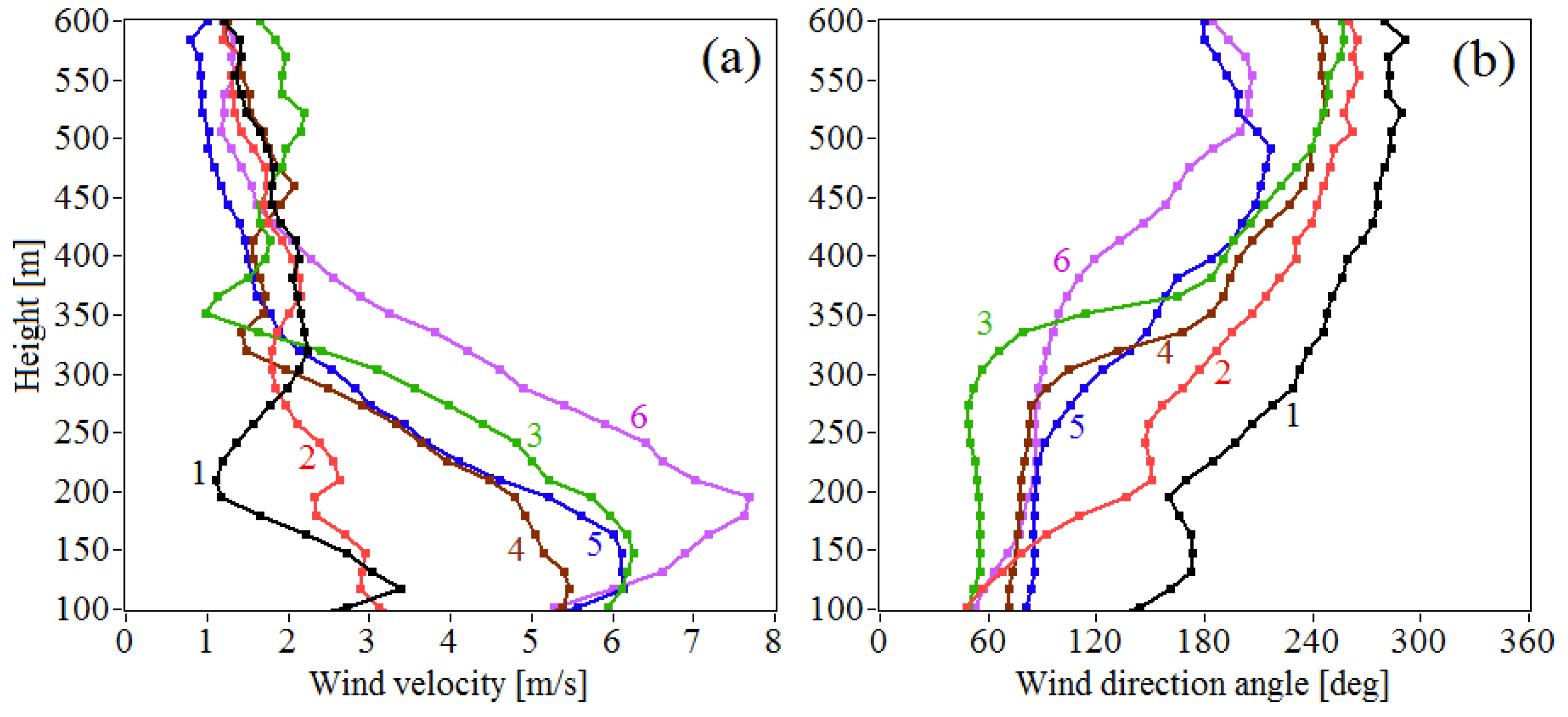
3.1. The IGW on 6 July 2021
On 6 July 2021, the IGW appeared after 03:00 local time (hereinafter, local time is indicated). As can be seen in
Figure 1, LLJ with a maximum wind speed at a relatively low height begins to form at approximately the same time. This process is accompanied by a sharp change in the wind direction starting from a height of 300 m, which becomes the opposite above 500 m (
Figure 1b).
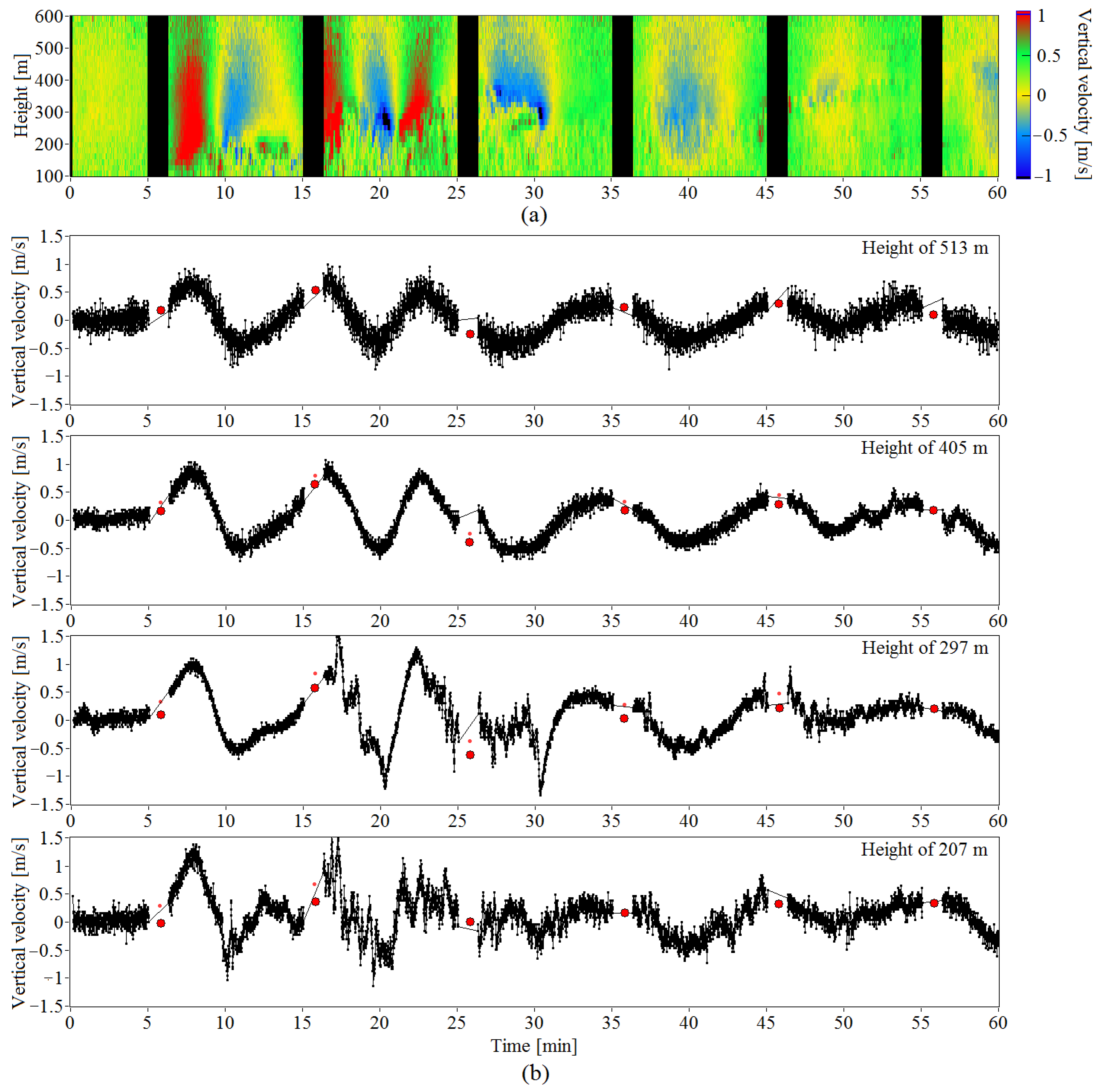
Figure 2a shows the height–time distribution of the vertical component of wind velocity
. The black color means no data since conical scanning by the probing beam was carried out at that time.
Figure 2b shows the time series of the vertical velocity at different heights as obtained from the distribution in
Figure 2a. The red circles in
Figure 2b are for the estimates of the vertical velocity
determined from conical scanning data. These estimates are in good agreement with the time series
shown by the black curves in
Figure 2b. It follows from
Figure 2 that the IGW appeared at approximately 03:06 LT in the atmospheric layer of 100–600 m. This IGW caused oscillations of the vertical velocity with an amplitude
up to 1 m/s (at a height of 405 m) in the initial period.
Within an hour, the amplitude gradually decreased, while the period of oscillations increased by almost 1.5 times. At heights of 405 and 513 m, where the wind turbulence is weak, variations of the vertical velocity have the form of quasi-harmonic oscillations. Uncorrelated random dribbling of the time series at these heights is associated with instrumental error, which increases with height due to a decrease in the . In the low layers (in particular, at heights of 297 and 207 m), random deviations of due to wind turbulence are quite significant and lead to a distortion of the quasi-harmonic form of wind velocity oscillations.
Figure 3a shows the time series of the vertical component of wind velocity
at a height of 405 m in the period from 02:00 to 06:00 LT. One can see that the IGW that appeared at 03:06 decayed gradually over almost two hours until IGW energy was completely converted into the energy of turbulent wind velocity variations.
To determine the frequency
of quasi-harmonic oscillations of wind velocity (oscillation period
) induced by IGW propagation, we used the data in
Figure 3a at non-overlapping time intervals of 03:06–03:26 and 03:26–03:46 LT shown in
Figure 3a by the blue and red arrows, respectively. From the data for
at these intervals, after uniform interpolation and the addition of the corresponding number of zeros to each of the velocity arrays, we obtained two power spectra of vertical velocity variations. These spectra are shown in
Figure 3b. From the position of the maximum of each of these spectra (see the brown vertical lines in
Figure 3b), we found that the frequency was
= 0.0021 Hz (period
8 min) in the interval of 03:06–03:26 and
= 0.0015 Hz (period
11 min) in the interval of 03:26–03:46.
The only parameter characterizing the spectra of the turbulent field of velocities in the inertial frequency range is the TKE dissipation rate
. The larger the SNR, the smaller the error of
estimation from lidar velocity measurements. To minimize the errors in estimating the spectra of turbulent fluctuations of the vertical velocity, we used the data in
Figure 2b for the time series
at a height of 297 m. This height nearly coincides with a height of 300 m, at which the SNR is maximal as follows from the height–time distribution of the
obtained from the measurements by the StreamLine lidar on 6 July 2021. A height of 300 m corresponds to the distance that the probing beam was focused at. Thus, the instrumental error
of estimation of the vertical wind velocity
and, consequently, the relative errors of estimation of the dissipation rate and the spectrum are minimal. The spectra
were calculated by Equation (1) for four 30 min intervals, whose boundaries are shown by the black arrows in
Figure 3a. The results are shown as black curves in
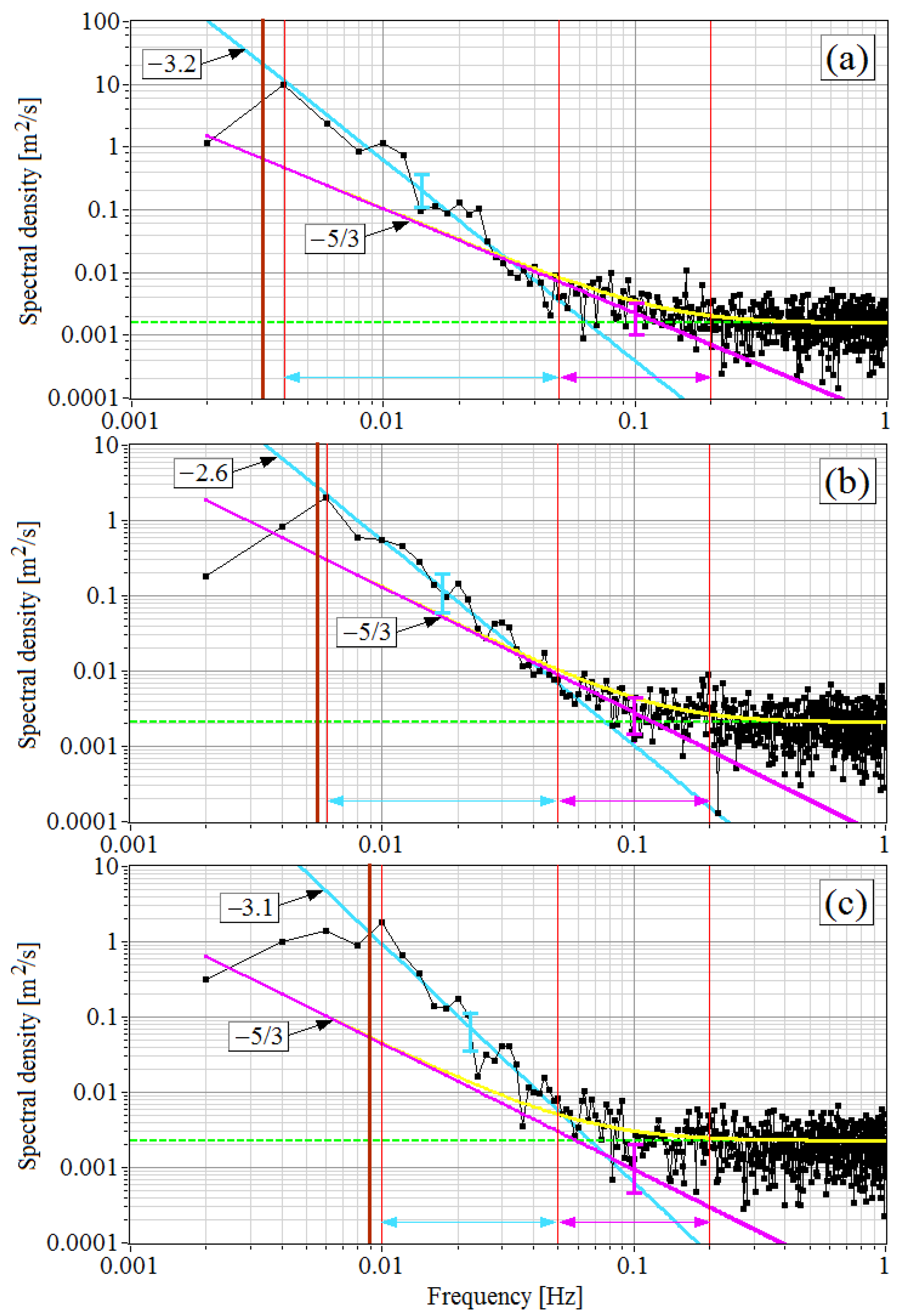
Figure 4.
As in
Figure 3a, the vertical brown lines in
Figure 4 show the frequencies
of IGW-induced velocity oscillations determined in the same way as described above. There is no such line in the spectrum calculated for the first interval of 02:36–03:06 because the IGW has not yet appeared at that time. The spectra within the frequency
range from 0.05 to 0.2 Hz (shown by the red arrows in
Figure 4) were used to estimate the TKE dissipation rate
by the method proposed in [
46]. It can be seen that as the IGW appears, the spectral amplitude nearby the frequency
increases by more than two orders of magnitude. As a consequence, the variance of the vertical wind velocity
calculated by Equation (2) as a sum of amplitudes at frequencies
0.002 Hz increases as well. The lower boundary
= 0.05 Hz of the frequency range, within which the dissipation rate is determined, is far higher than
(approximately 25 times higher). Nevertheless, the IGW also leads to an increase in the dissipation rate
. An increase in the spectrum amplitude by an order of magnitude within the turbulence inertial range (purple lines) is clearly seen in the two lower figures compared to the upper figures in
Figure 4. This is likely due to the partial transfer of IGW energy to small-scale turbulent variations of the vertical component of wind velocity.
Figure 5 shows the height–time distributions of the instrumental error of estimation of the radial velocity
, the variance of the vertical wind velocity
, the TKE dissipation rate
, and the relative error of estimation of the dissipation rate
with a height step of 18 m and a time step of 10 min. These distributions were obtained from measurements by StreamLine lidar from 00:00 to 12:00 LT on 6 July 2021. The black color in
Figure 5d means that
exceeds the level of 50%. The white rectangles show the boundaries of the height–time domain, in which the IGW was observed. One can see that the dissipation rate
and the variance of the vertical velocity
that characterize the intensity of wind turbulence have larger values in this domain than outside it.
3.2. The IGW on 28 May 2022
On 28 May 2022, the IGW emerged during a rather strong low-level jet at 02:30 and lasted until 05:30 LT.
Figure 6 shows the vertical profiles of the horizontal wind velocity obtained in this interval. It can be seen that the height of the maximum velocity (LLJ center) decreased from 350 to 240 m in 2.5 h. The IGW was observed only in the top part of the jet, while below the center of the LLJ, there was quite intense turbulent air mixing.
The height–time distribution of the vertical wind velocity in the period from 02:00 to 05:00 LT on 28 May 2022 is shown in
Figure 7a. As in
Figure 2a, the black color shows the time intervals, in which conical scanning by the probing beam was carried out to determine the wind speed
and the wind direction angle
. In
Figure 7a, we can see oscillations of the vertical velocity at heights from 250 to 450 m that are caused by the IGW propagating in this layer. Below 250 m, turbulent velocity fluctuations that are quite intense for the nighttime are observed.
Figure 7b shows the time series of the vertical wind velocity at a height of 351 m drawn from the data in
Figure 7a. It follows from
Figure 7b that the amplitude of quasi-harmonic oscillations of the vertical velocity does not exceed 0.8 m/s.
After applying low-pass filtering and spline interpolation of data with a uniform rather small time step to the time series shown in
Figure 7b and dividing it into six 30 min intervals, we calculated the temporal spectra for each interval. The positions of maxima in these spectra were used to determine the frequencies
and calculate the periods
of quasi-harmonic oscillations of the vertical velocity.
Figure 7c shows how the oscillation period changed during IGW passage. It can be seen that
decreased with time from approximately 6 min down to almost 1 min.
Using the data in
Figure 7b, we calculated the spectra of turbulent fluctuations of vertical velocity
for different time intervals. Three of these spectra are shown in
Figure 8. The brown vertical lines show the frequencies of oscillation
corresponding to the periods
in
Figure 7c. We can see that the frequency
increases with time (compare (a), (b) and (c) in
Figure 8 between themselves). The IGW leads to an increase in the amplitude of the spectrum
in the frequency range from
to 0.05 Hz. Thus, the slope of the spectrum in this range becomes larger than the slope of the spectrum with the −5/3 power-law frequency dependence
.
To characterize the spectra in the frequency range from
to 0.05 Hz, we assume that the spectra of the vertical velocity averaged over an ensemble of realizations
are characterized by power-law dependence
, where
is the frequency-independent coefficient and
is the exponent. Then, through the least-square fitting of the linear dependence
on
to
within this interval, we find
and
and approximate the experimental spectra by the power-law frequency dependence. In
Figure 8, the obtained frequency functions
are shown by blue lines with an indication of the exponent:
= −3.2 (
Figure 8a),
= −2.6 (
Figure 8b), and
= −3.1 (
Figure 8c). These estimates of
differ significantly from −5/3 and are relatively close to the Lumley–Shur theoretical value
= −3 and the −3 frequency dependence in the low-frequency range of the turbulent spectra in the SBL [
43].
The same method was used to estimate the exponent
of the spectrum in the frequency range of 0.006–0.05 Hz for the time interval from 00:00 to 08:00 LT on 28 May 2022 with a 10 min step from lidar measurements at a height of 351 m. The obtained time series
is shown as a black curve in
Figure 9a. The time series of the Richardson number calculated from the lidar data on the wind velocity and from the temperature profiler data with the same time step is shown in
Figure 9b. It follows from
Figure 9b that the temperature stratification was stable at a height of 351 m in the considered period, and the Richardson number was
Ri > 0. According to the temperature data, stable stratification in the boundary layer above 200 m was observed starting from 20:00 LT on May 27. It can be seen in
Figure 9b that before the IGW appeared at 02:30 and after IGW destruction, starting from 05:00 LT, the Richardson number exceeded the values of
Ri observed during IGW propagation from 02:30 to 05:00 LT by one to two orders of magnitude. In
Figure 9a, we can see that before and after the IGW, the exponent
exceeds −5/3 and ranges approximately within −0.7 >
> −1.5. This is consistent with the variability range of the slopes of the temporal spectra of wind velocity components observed during stable stratification in the atmospheric surface layer in the Arctic [
7]. During IGW propagation from 02:30 to 05:00 LT, the exponent
becomes less than −5/3 and falls in the range of −2.5 >
> −3.5. During IGW passage,
averages –3.
Figure 10 shows the height–time distributions of
,
,
, and
obtained from 24 h lidar measurements on 28 May 2022. The white rectangle bounds the domain of IGW observation. It can be seen that for most of this domain, the relative error in estimating the TKE dissipation rate does not exceed 30%. The dissipation rate in this domain varies from
m
2/s
3 to
m
2/s
3, and it does not exceed 10
−5 m
2/s
3 in 75% of cases and 10
−6 m
2/s
3 in 50% of cases.
3.3. The IGW on 30 May 2022
On 30 May 2022, the IGW was observed in the period from 04:00 to 07:40 LT.
Figure 11 depicts the spectra of the vertical wind velocity component obtained from lidar measurements at different heights during the propagation of the IGW with
0.003 Hz in the atmospheric layer of 250–600 m. To avoid the influence of the noise spectral component
, we determined the exponent
within the frequency range from 0.004 to 0.02 Hz. The figure clearly illustrates the significant excess of the spectrum slope (blue lines) over the −5/3 slope (purple lines) for heights starting from 297 m.
Figure 12 depicts the vertical profiles of the horizontal wind velocity
, TKE dissipation rate
, relative error of lidar estimation of the dissipation rate
, exponent
, temperature
, and Richardson number
. It follows from
Figure 12e,f that during the measurements at heights of 100–600 m, the temperature stratification in the boundary layer is stable, the temperature
increases with height, and the Richardson number is positive
> 0. In the height range of 100–250 m, where the IGW effect is insignificant,
does not exceed unity, and the exponent
> −5/3. The range of exponent variation at heights of 100–250 m is −0.2 >
> −5/3, which is consistent with the values of
in
Figure 9a in the absence of the IGW. Starting from a height of 250 m, where the IGW effect is already noticeable,
increases fast and achieves 300 at heights of 400–500 m, where the IGW effect is maximal (see
Figure 11). Simultaneously, the exponent
decreases sharply starting from a height of 250 m. At heights of 400–550 m, where the IGW energy is maximal, the exponent is
.
4. Discussion
The continuous lidar measurements were conducted in different periods from May to July of 2020, 2021, and 2022 within 53 days in total. During this time, we observed 23 events of IGW that arose at night and in the morning (from 02:00 to 08:00 local time). In approximately half of the events, the duration of IGW-induced continuous quasi-harmonic oscillations of the vertical velocity ranged from 0.5 to 5 h. The total duration of their observation was 25 h. The waves were observed in a stably stratified ABL at heights from 200 to 600 m.
In the overwhelming majority of cases, IGWs in a stably stratified boundary layer occur during LLJs. The ratio of the total duration of the LLJ observed during the measurements to the total lifetime of the IGW that occurred during the LLJ is approximately 4.3. During the measurements, only two cases of IGW formation in the absence of a jet were revealed. This happened when the wind speed did not exceed 3 m/s, and the wind direction alternated sharply to the opposite direction with height. We can assume that the vertical inhomogeneity of wind in the velocity (LLJ) or direction is one of the reasons for IGW generation in the SBL.
Using the results of lidar measurements during the propagation of IGWs in the atmospheric boundary layer, we calculated 700 spectra of the vertical component of the wind velocity : 220 spectra from measurements in 2020, 155 spectra from measurements in 2021, and 325 spectra from measurements in 2022. The spectra were calculated for the periods of IGW propagation, with a time step of 15 min and a height step of 18 m in an altitude range from 200 to 600 m.
All the spectra were estimated from 30 min measurements of the vertical wind velocity under the following conditions: (1) the IGW observed during the entire 30 min measurement interval, (2) the height not below the LLJ center (height of the maximal horizontal wind velocity ), (3) IGW frequency not higher than 0.02 Hz, (4) the not lower than −18 dB, (5) and stable temperature stratification.
For each spectrum, the exponent
was calculated assuming the power-law dependence on frequency in the low-frequency region. When determining
from the selected spectra
, we set the upper boundary of the frequency range, within which
was estimated, depending on the level of the noise component of the spectrum (not lower than 0.02 Hz and not higher than 0.06 Hz). The lower boundary of the frequency range was taken to be not lower than the frequency of IGW-induced oscillations of the vertical velocity
.
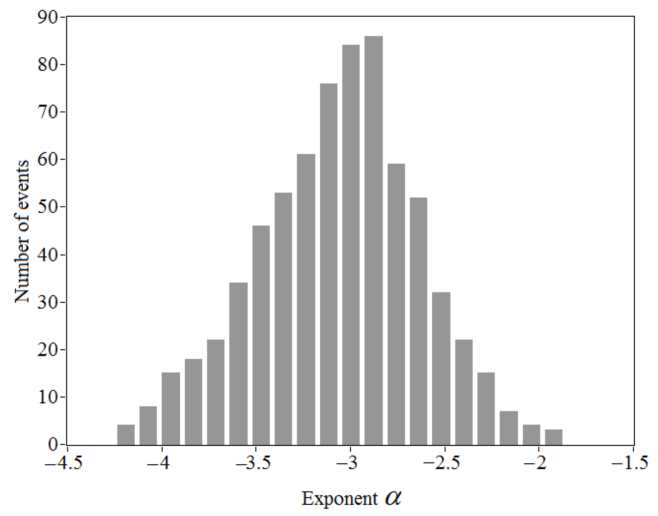
Figure 13 shows the histogram of all the obtained estimates of
. It follows from the data in
Figure 13 that the average value of the exponent is
= −3, while the standard deviation of the estimates is 0.44. The probability that the estimate of the exponent
takes a value from −3.5 to −2.5 is 80%. The obtained estimate of the average exponent confirms “−3” low frequency slope caused by IGWs in turbulent spectra, which were observed in the 300 m lower layer of the SBL [
43].
We believe that in accordance with the terminology [
55], we observed buoyancy IGWs that appear much less often than Kelvin–Helmholtz [
44] ones. In each specific event of such type of IGW, the low-frequency slope of the turbulent spectrum can significantly deviate from that which is determined by the average exponent
= −3. The histogram in
Figure 13 gives the values and corresponding probabilities of these deviations.
5. Conclusions
The paper presents experimental data and results of the study of wave turbulence interactions in the stable atmospheric boundary layer. The analysis was based on the data of lidar measurements of the vertical component of wind velocity during IGW propagation with the use of temperature data of the microwave radiometer in the spring–summer periods of 2020–2022 in Tomsk, Russia. The results obtained allow us to draw the following conclusions.
In the overwhelming majority of cases, IGWs in a stably stratified boundary layer occur during LLJs. During the measurements, only two cases of IGW formation in the absence of a jet were revealed. This happened when the wind speed did not exceed 3 m/s, and the wind direction alternated sharply to the opposite direction with height. It is possible that the vertical inhomogeneity of the wind in the velocity (LLJ) or in the direction is one of the reasons for IGW generation in the SBL.
With the appearance of the IGW, the amplitude of the spectrum of turbulent fluctuations in the vertical component of the wind velocity increases significantly, sometimes by orders of magnitude, in the vicinity of the frequency of the IGW-induced quasi-harmonic velocity oscillations compared to the spectral amplitudes at these frequencies in the absence of the IGW. This leads to an increase in the variance of fluctuations of the vertical velocity during the IGW, which is the sum of spectral amplitudes in the entire frequency range. IGW energy is transferred to small-scale turbulence. As a result, the slope of the spectrum of vertical velocity in the low-frequency range between the frequency of IGW-induced oscillations and the frequency of the lower boundary of the inertial range exceeds the slope corresponding to the −5/3 power-law frequency dependence of the spectrum. IGW energy is transferred into the inertial interval of turbulence as well. The amplitude of the spectrum in the inertial frequency range may increase by an order of magnitude due to an increase in the TKE dissipation rate during the IGW.
A total of 700 spectral estimates obtained in the measurements show that during the IGW, the spectra of the vertical velocity in the low-frequency range between the frequency of IGW-induced oscillations and the frequency of the lower boundary of the inertial range obey the power-law frequency dependence, with the exponent ranging from −4.2 to −1.9. Eighty percent of estimates fall within the range from −3.5 to −2.5. The average value of the exponent is = −3, which is consistent with a low-frequency slope caused by IGWs in turbulent spectra in a lower layer of the SBL. We believe that in this study, we observed buoyancy IGWs that appear not often. In each specific event of such type of IGW, the low-frequency slope of the turbulent spectrum can significantly deviate from that which is determined by the average exponent = −3. The accumulated database of the exponent of the spectra power-law frequency dependencies gives the values and corresponding probabilities of these deviations.


