Article

Robust Loop Closure Selection Based on Inter-Robot and Intra-Robot Consistency for Multi-Robot Map Fusion

1
School of Surveying and Geo-Informatics, Tongji University, Shanghai 200092, China
2
Department of Computer Science and Technology, School of Electronics and Information Engineering, Tongji University, Shanghai 201804, China
3
The Key Laboratory of Embedded System and Service Computing, Ministry of Education, Tongji University, Shanghai 201804, China
4
Institute of Intelligent Vehicle, Tongji University, Shanghai 201804, China
*
Author to whom correspondence should be addressed.
Remote Sens. 2023, 15(11), 2796; https://doi.org/10.3390/rs15112796
Submission received: 23 April 2023 / Revised: 15 May 2023 / Accepted: 20 May 2023 / Published: 27 May 2023

Abstract

:
In multi-robot simultaneous localization and mapping (SLAM) systems, the system must create a consistent global map with multiple local maps and loop closures between robot poses. However, false-positive loop closures caused by perceptual aliasing can severely distort the global map, especially in GNSS-denied areas, where a good prior of relative poses between robots is unavailable. In addition, the performance of the consistency metric in existing map fusion methods relies on accurate odometry from each robot. However, in practice, cumulative noise is inevitably present in robot trajectories, which leads to poor map fusion with existing methods. Thus, in this paper, we propose a robust consistency-based inter-robot and intra-robot loop closure selection algorithm for map fusion. We consider both pairwise-loop consistency and loop-odometry consistency to improve robustness against false-positive loop closures and accumulative noise in the odometry. Specifically, we select a reliable inter-robot loop closure measurement with a consistency-based strategy to provide an initial prior of relative pose between two robot trajectories and update the pose variables of the robot trajectories. The loop closure selection problem is formulated as a maximum edge weight clique problem in graph theory. A performance evaluation of the proposed method was conducted on the ManhattanOlson3500, modified CSAIL and Bicocca datasets, and the experimental results demonstrate that the proposed method outperforms the pairwise consistency measurement set maximization method (PCM) under severe accumulative noise and can be integrated with M-estimation methods.

1. Introduction

In multi-robot simultaneous localization and mapping (SLAM) systems, each robot explores its local environment, creates a map from its observations, and estimates its own position within that map. Multi-Robot SLAM addresses the efficiency issue in scenes of a large area, e.g., underwater scenes [1]. However, the individual maps created by each robot may have inconsistencies due to different sensor measurements and environmental conditions. Thus, it is necessary to estimate the relative pose between the maps of multiple robots so that the individual maps can be merged into a consistent global map. This task is known as map fusion [2].
The simplest way to accomplish this task is to align each map to a same global reference, e.g., by using a global navigation satellite system (GNSS). However, in GNSS-denied areas, e.g., indoor environments and urban canyons, direct measurements of other robots’ poses or indirect measurements from similar landmarks must be utilized [2]. Similar to the single-robot map estimation problem, these measurements are frequently treated as loop closures and represented by factor nodes added to a global factor graph. Under the assumptions of independent measurement and Gaussian noise, the factor graph can be solved as a nonlinear least squares problem [3]. Thus, map fusion is realized. Map fusion is critical to the success of multi-robot SLAM, because it allows the robots to share their knowledge of the environment and create a more accurate and comprehensive map than any individual robot could create alone. The resulting global map can be used for a variety of applications, such as path planning, obstacle avoidance, and localization.
However, several issues must be considered in the map fusion problem. First, the prior of relative pose between robots may not exist [4] in multi-robot SLAM. This requires the map fusion algorithm to either function without the prior information or calculate a reliable prior by itself. Second, perceptual aliasing introduces a false-positive inter-robot loop closure to the system, which reduces the performance of the maximum likelihood estimator drastically [5]. Third, each robot’s trajectory estimate can have errors due to sensor noise and drift, and we found that poor single-robot odometry can result in poor map fusion performance, and to the best of our knowledge, this issue is rarely discussed in previous studies. In contrast, many existing map fusion methods assume high-quality single-robot trajectories [2,4]. As a result, these methods exhibit significant performance degradation as the accumulative noise in the odometry increases.
Thus, in this paper, we propose a robust consistency-based inter and intra-robot loop closure selection algorithm for multi-robot pose graph map fusion. Specifically, we create a novel measurement consistency score that integrates pairwise-loop consistency and loop-odometry consistency, which improves robustness against false-positive loop closures and accumulative noise in the odometry. Utilizing the pairwise-loop consistency from the consistency metric, an initial inter-robot loop closure can be selected with acceptable increases in computational costs. In addition, the initial loop closure allows us to update the pose estimates and to calculate the full consistency metric for both inter-robot and intra-robot loop closures. Finally, the loop closure selection problem is formulated and solved as a maximum edge weight clique problem.
Our primary contributions are summarized as follows:
1
We present a novel consistency score that considers both pairwise-loop and loop-odometry consistency for loop closure selection;
2
We propose an efficient consistency-based loop closure selection strategy to provide an initial relative pose estimate between robots;
3
To the best of our knowledge, this work is the first to conduct experiments to demonstrate the impact of accumulative noise on multi-robot map fusion problem, and our experimental result shows that the existing loop selection method relies on the quality of single-robot odometry and degenerates significantly under severe accumulative noise.

2. Related Work

2.1. Robust Optimization in SLAM

Pose graph optimization (PGO) is commonly used as the estimation backbone in state-of-the-art SLAM systems [6]. However, the standard least squares formulation of PGO is not robust against corrupted observations, which can cause the estimator to diverge from the actual value of the parameters to be solved. In practical SLAM applications, these corrupted observations arise from perceptual aliasing, which further leads to erroneous data associations and wrong measurement constraints.
To address this issue, robust optimization techniques are designed to handle outliers and noise in the SLAM problem. Robust SLAM estimation methods can be categorized into two classes [5]. The first class focuses on identifying the inlier measurement set by searching for the best subset that satisfies a mutual consistency metric. Ref. [7] used random sampling to iteratively decide inliers and outliers. Ref. [8] divided measurements into small groups and evaluated the consistency within and between the groups. Ref. [4] designed pairwise consistency measurement set maximization (PCM) and enforces pairwise internal consistency to inlier measurement sets.
The other class, which is referred to as M-estimation, replaces the likelihood function in the standard maximum likelihood estimation (MLE) with robust losses that are less sensitive to outliers. An early representative method is the popular Huber loss [9]. Ref. [10] discarded incorrect loop closure candidates using switchable variables and functions. Ref. [11] improved [10] by dynamically scaling the information matrix of each non-incremental edge. Ref. [12] used the Gaussian mixture model to represent the non-Gaussian behaviors of loop closures and employed max-mixture instead of sum-mixture to solve the problem efficiently. However, robust cost functions typically introduce non-convexities, which make the objective function more susceptible to converge to poor quality critical points [5]. Refs. [13,14] used convex relaxation to solve SLAM problems with robust cost functions. Ref. [15] further formulated the M-estimation problem and outlier procedure as a dual problem with Black-Rangarajan duality and solved the SLAM problem using graduated non-convexity optimization (GNC).

2.2. Robust Optimization in Multi-Robot SLAM

The majority of methods in Section 2.1 are designed for a single-robot pose graph and fails in multi-robot scenarios due to the lack of reliable initialization [10,11,12] or trusted odometry [8].
Previous studies [16,17] used expectation maximization to determine inliers and outliers from a set of measurements, which provides initial estimates for the relative poses between multiple robots. PCM [4] is widely adopted as an outlier rejection method in multi-robot systems [18,19,20,21]. Ref. [2] further added data similarity to the consistency weight and reformed PCM as a maximum edge weight clique problem (MEWCP) rather than MCP. The weight formulation improves PCM’s performance when perceptual aliasing occurs while the cardinality of the true measurement set is small. Ref. [2] is the most similar method to our proposed method. However, the method does not consider the consistency between loop closures and odometry, and it required similarity input from the front end, specifically, the number of features matched and the tuning parameter for loop closure. However, our method only depends on the pose graphs of multi-robots to function. On the other hand, we perform a consistency-based initialization and consider both inter-robot and intra-robot measurements in one framework.
Ref. [6] performed a distributed initialization by solving a robust pose averaging problem and then solved the distributed PGO with GNC (D-GNC). D-GNC showed better robustness against outliers and lower trajectory error; however, it depends heavily on the performance of initialization. In addition, the runtime of the GNC optimizer is much larger than that of PCM with heuristic solvers. Thus, an early stop must be employed in practical applications.

3. Preliminaries

3.1. Multiple Robot Pose Graph Optimization

Graph SLAM uses a graphical structure to represent the Bayesian SLAM [22]. In single-robot scenarios, the pose graph optimization (PGO) can be formulated as the following MLE problem:
X ^ = arg max X P ( Z o , Z l | X )
where X is the set of all S E ( n ) pose variables x t , which denotes the robot trajectory, and Z o and Z l are two sets of measurements z i j , representing the relative pose constraints between x i and x j : Z o denotes the odometric measurement set where i and j are consecutive, and Z l denotes the loop closure measurement set. Note that Z o and Z l have empty intersection, and together they make up the full set of measurements.
The multi-robot pose graph optimization is an extension of the single-robot PGO problem, where both inter-robot and intra-robot loop closures can be obtained. Here, the relative pose between the local coordinate frames of multiple robots is unknown and must be estimated, as is suggested in [23]. As a result, the multi-robot map fusion problem (we consider two robots in this example) can be expressed as follows:
X ^ , T ^ g = arg max X , T g P ( Z o a , Z o b , Z l a , Z l b , Z l a b | X , T g )
where T g = { T g a , T g b } , representing the relative transformation between the respective robot’s local frame a , b and the global reference frame g. Here, Z o a , Z o b , Z l a , and Z l b represent the intra-robot measurements sets, and Z l a b is the inter-robot loop closure measurements set.

3.2. Loop Closure Selection Problem

Loop closure selection is a crucial step in SLAM algorithms that involves identifying and selecting the most significant loop closures in the map to refine the robot’s estimated trajectory and improve the accuracy of the map. The selection of loop closure is based on consistency because it is difficult to determine whether a measurement is an inlier or outlier [24]. We adopt the definition of pairwise internal consistency set [4] to make sure that every selected measurement be consistent with all the other selected measurements. Given a set of measurements Z ˜ , the condition of pairwise internal consistency can be formulated with a consistency metric C and the threshold γ as follows:
C ( z i , z j ) γ , z i , z j Z ˜
where C is a function measuring the consistency of measurements z i and z j .
Assumption 1. 
True loop closure measurements are more likely to have a higher degree of pairwise consistency metric scores than false positive loop closure measurements [2].
Assumption 1 indicates a larger metric magnitude from true loop closures and is robust against cases where the size of the true loop closure measurement set is smaller than that of the false positive loop closure measurement set.
Based on this assumption, the best loop closure measurement subset can be selected using the following equation:
Z ˜ * = arg max Z ˜ Z l z i , z j Z ˜ C ( z i , z j )
where Z l = Z l a Z l b Z l a b . Z ˜ * is the selected loop closure measurement subset.

4. Methodology

The proposed loop closure selection method relies on an initialization procedure, a novel pairwise consistency metric, and a graph-based solution. In this section, our novel pairwise consistency metric is first defined. Then, a single loop closure is selected with a simple strategy to provide an initial pose estimate between robots. Finally, the graph theory algorithm leveraged to solve the loop closure selection problem is introduced. A diagram of the proposed algorithm is shown in Figure 1, where the cyan blocks show our main contributions. In the following, we consider a case with two robots as an example.

4.1. Inter and Intra-Robot Consistency Metric

In the procedure of multi-robot SLAM, odometry of each robot, inter-robot loop closures and intra-robot loop closures are obtained. The pose graph formulation of the concerned measurements is shown in Figure 2. The odometry of each robot is represented by triangles of different colors.
Pairwise consistency metric measures the consistency between pairs of observations or measurements, and checks if the consistency between measurements is within certain thresholds. The proposed pairwise consistency metric is expressed as follows:
C ( z i k p q , z j l r s ) = c l l ( z i k p q , z j l r s ) c l o ( z i k p q , x ^ i k p q ) c l o ( z j l r s , x ^ j l r s ) , p , q , r , s { a , b }
where z i k p q represents the loop closure measurement between the ith frame of robot p and the kth frame of robot q, and x ^ i k p q represents the relative pose estimation between the ith frame of robot p and the kth frame of robot q. Note that in the single-robot scenario, the pose estimate is usually obtained from odometry measurements. However, in the case of multiple robots ( p q or r s ), relative pose estimates are not available directly because the relative pose between robots is initially unknown; this issue will be settled in Section 4.2. c l l represents the geometric consistency between two loop closures, z i k p q and z i k r s . c l o represents the geometric consistency between one loop closure and the pose estimation of the corresponding odometry. Specifically, these three terms can be expressed as:
c l l ( z i k p q , z j l r s ) = exp ( | | ( z i k p q ) x ^ i j p r z j l r s x ^ l k s q | | Σ )
c l o ( z i k p q , x ^ i k p q ) = exp ( | | ( z i k p q ) x ^ i k p q | | Σ )
c l o ( z j l r s , x ^ j l r s ) = exp ( | | ( z j l r s ) x ^ j l r s | | Σ )
where ⊕ represents pose composition and ⊖ represents pose inversion [25]. In addition, | | · | | Σ refers to the Mahalanobis distance.
c l l in Equation (6) (referred to as pairwise-loop consistency) was used as the consistency metric in previous studies [2,4], and its value is proportional to the probability density that the four rigid-body transformations actually form a cycle [26].
c l o in Equations (7) and (8) are referred to as the loop-odometry consistency, and their values are proportional to the probability density, causing the transformation of one loop closure and the corresponding odometry to actually form a cycle.
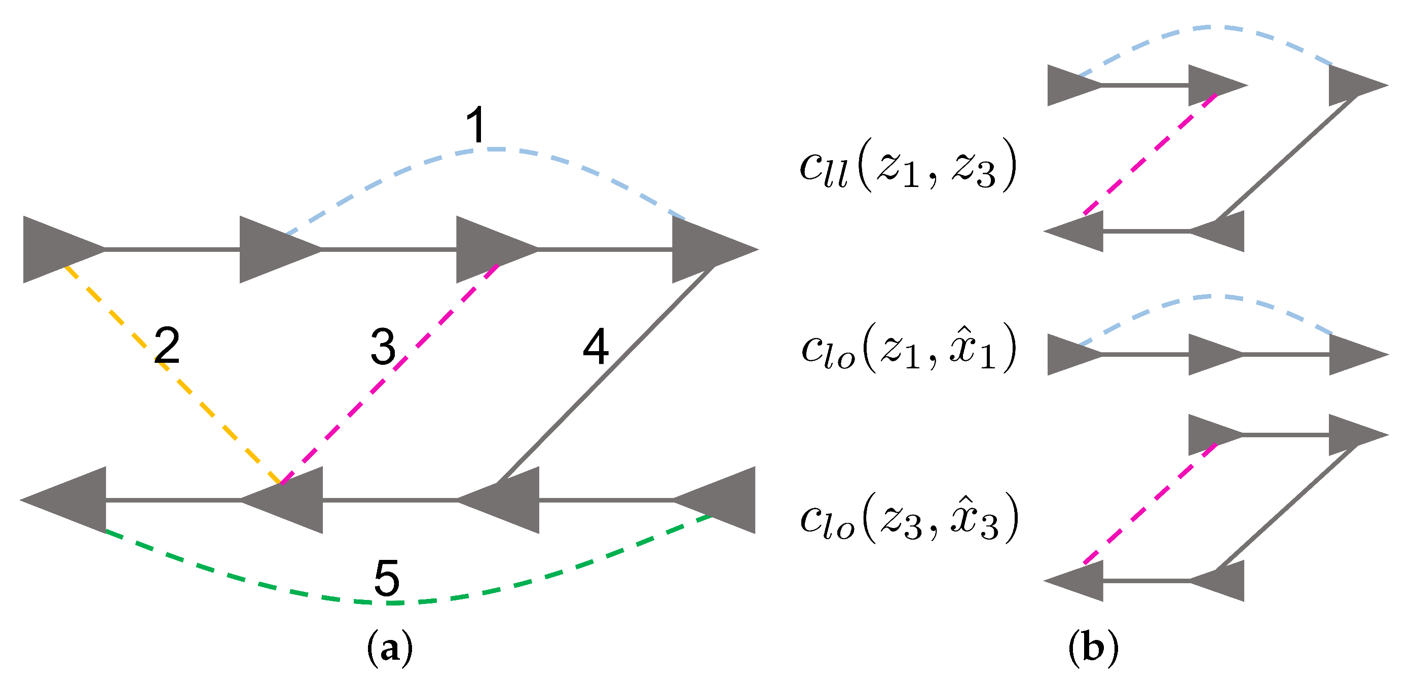
A simplified illustration of our proposed metric is shown in Figure 3.
Note that pairwise-loop consistency may degrade as the quality of the odometry decreases. When the current pose estimates x ^ i j p q and x ^ l k s q in Equation (6) are accurate, the pairwise-loop consistency score of two true loop closures is close to 1 and passes the threshold. In this case, the loop closure pair can be considered as inlier candidates. However, in practical applications, x ^ i j p q and x ^ l k s q can suffer from large error due to accumulative odometry noise, especially when i and j or l and k are distant in the robot trajectories. Large errors in pose estimates result in low pairwise-loop consistency scores and can potentially cause the rejection of true loop closures.
Thus, the loop-odometry consistency terms are integrated into an overall metric to reward the loop closure pairs, whose corresponding x ^ i j p r and x ^ l k s q are more likely to be accurate. Thus, we obtain the following:
x ^ i j p r = x ^ i k p q x ^ k j q r
x ^ l k s q = ( x ^ k j q r x ^ j l r s )
By omitting x ^ k j q r , we turn to a similar problem that determines whether x ^ i k p q and x ^ j l r s are likely to be accurate. Here, an approximate evaluation of the odometry’s quality can be realized by utilizing the loop-odometry consistency given in Equations (7) and (8).

4.2. Consistency-Based Initialization

The calculation of the proposed consistency metric requires an initial pose estimate between robots, which is unavailable at the beginning of the problem. Moreover, a reliable initial estimate between robots allows us to initialize robot trajectories in the global reference frame, which has a positive impact on the effect of PGO. Thus, an initialization strategy is introduced in the following.
Based on Assumption 1, an inter-robot loop closure that is likely to be consistent with other inter-robot loop closures can be found:
arg max i j = 1 n c l l ( z i , z j ) , z i , z j Z a b , j i
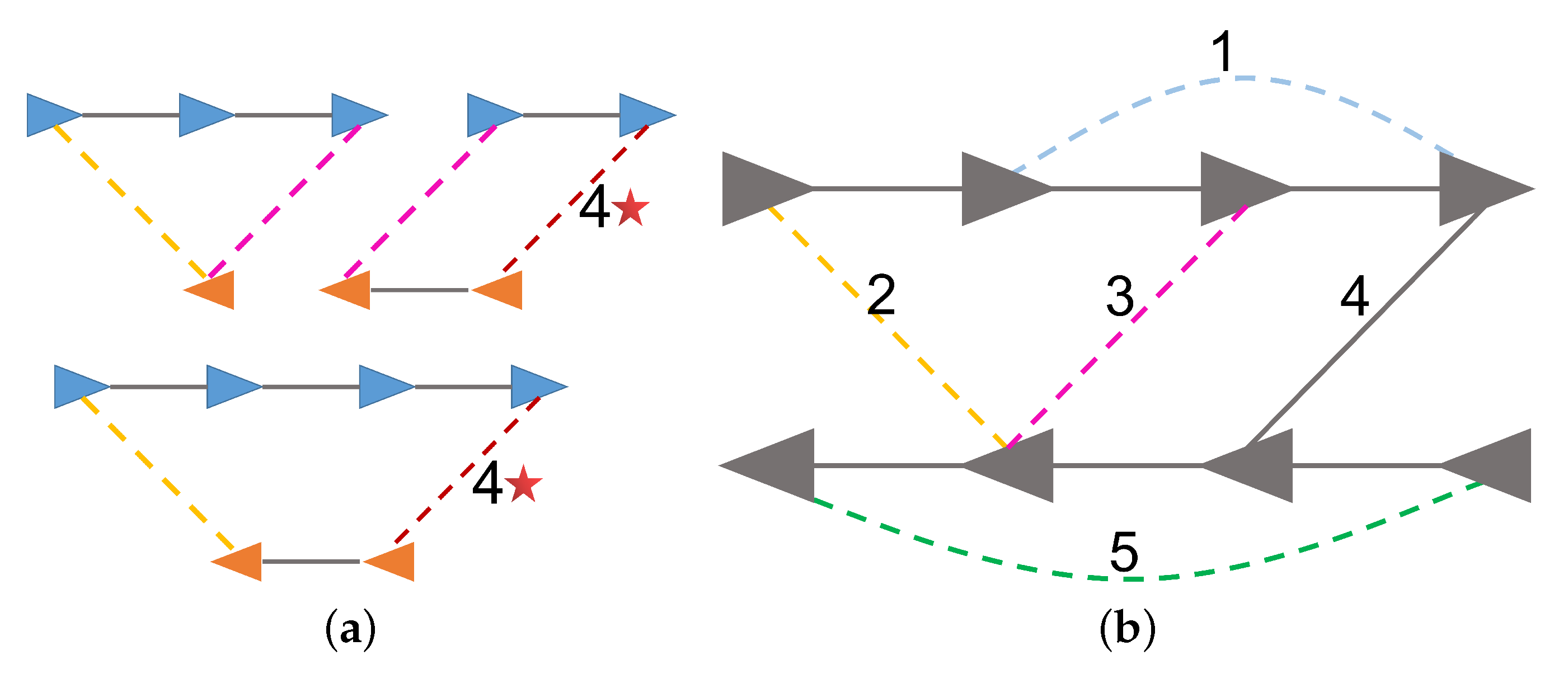
where n is the size of inter-robot measurements set Z a b . The selected inter-robot loop closure measurement z i , which is denoted z m n a b , is used as the initial relative pose between robots. A simplified illustration of our proposed initialization is shown in Figure 4.
Constrained by the selected loop closure measurement, pose variables of robot trajectories can be updated as follows:
X ^ , T ^ g = arg max X , T g P ( Z o a , Z o b , z m n a b | X , T g )
Note that this update does not change the pairwise-loop consistency terms in Equation (11) because the “shape” of each robot’s initial trajectory is unchanged; however, the update improves the accuracy of the loop-odometry consistency terms.
The selected loop closure measurement serves as the initial pose estimate between robots; thus, the pose estimates between two arbitrary nodes from different robots, which are needed in the calculation of the proposed consistency metric, can be calculated as follows:
x ^ p q a b = x ^ p m a a z m n a b x ^ n q b b
With Equation (13), the proposed consistency metric given in Equation (5) can be calculated.

4.3. Maximum Edge Weight Clique-Based Solution

The maximum edge weight clique problem is a graph optimization problem that involves finding the largest complete subgraph (clique) in a graph where the sum of the edge weights in the clique is maximized. Formally, the maximum edge weight clique problem can be defined as follows: Given an undirected weighted graph G = ( V , E ) , where V is the set of vertices and E is the set of edges, each edge is associated with a positive weight, where the goal is to find a subset C of V such that C forms a clique in G, and the sum of the weights of the edges in the induced subgraph of C is maximized.
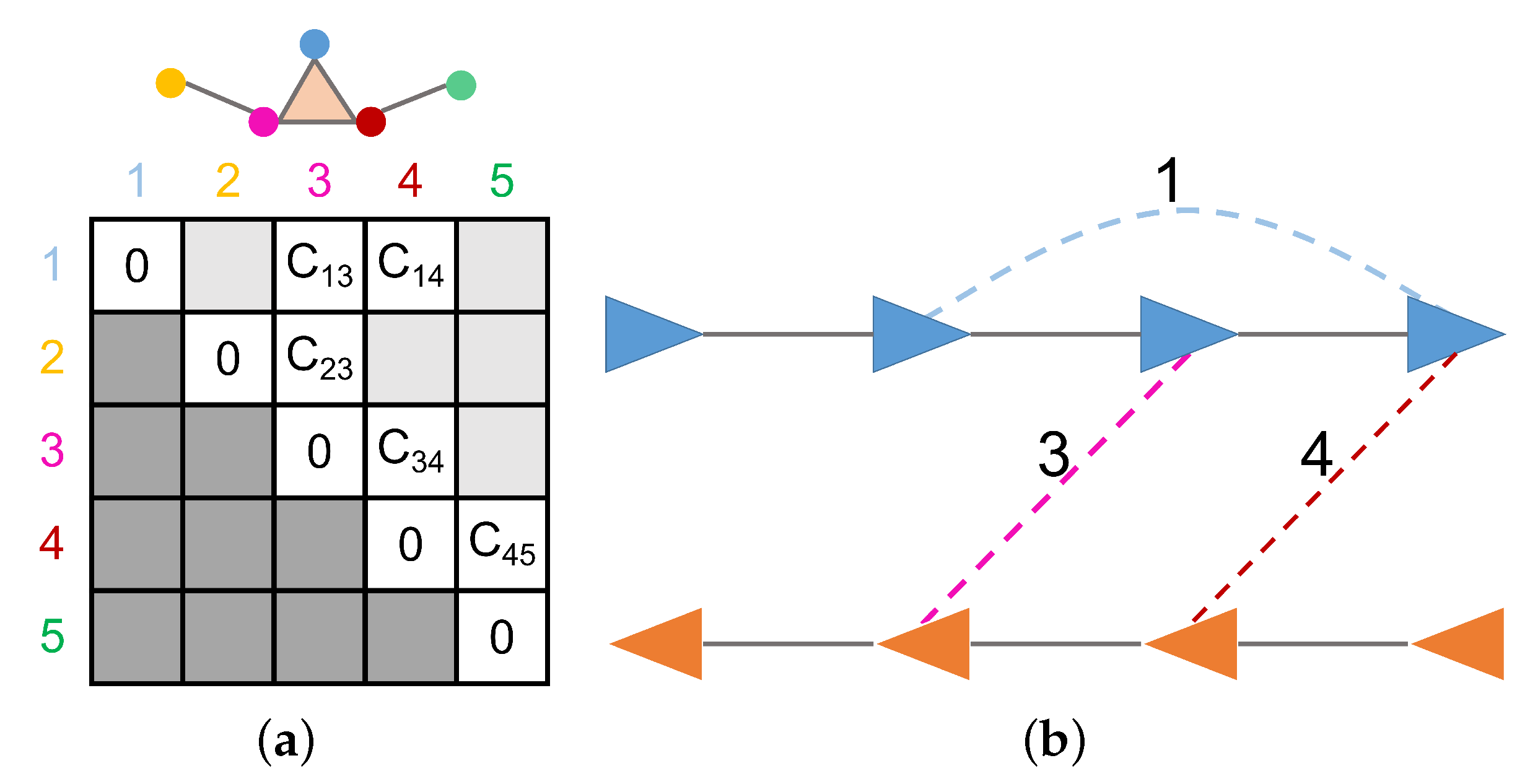
Equation (4) can be formulated as a maximum edge weight clique problem (MEWCP). The consistency metric C ( z i , z j ) of each loop closure pair is first calculated and stored in a symmetric matrix B, as shown in Figure 5. Each row or column of the matrix corresponds to one loop closure. Matrix elements that are less than the consistency metric threshold γ are changed into zeroes to symbolize that the corresponding loop closure pair does not fit the consistency condition. The diagonal elements are also filled with zeroes because the consistency between one loop closure and itself is meaningless. Note that this matrix shares the same form as the weighted adjacent matrix of an undirected weighted graph, where each vertice of the graph represents a loop closure measurement. Whether two vertices are adjacent corresponds to whether the loop closure measurement pair fits the pairwise consistency metric condition, and the weight of the corresponding edge refers to the pairwise consistency metric score of the loop closure measurement pair. Thus, finding a measurement subset that fits the pairwise internally consistent condition in Equation (3) with the greatest overall consistency metric is equal to finding a clique with the greatest edge weight sum. Therefore, the solution to the robust loop closure selection problem can be transformed into the following expression:
Z ˜ * = M E W C P ( B )
The MEWCP procedure is a classical combinatorial optimization problem that has been proven to be NP-hard. There are several approximation algorithms and heuristics that can provide good solutions in practice. Here, we utilize the ReConSLS solver [27] due to its simplicity, efficiency, and open-source implementation.
Finally, the multi-robot map fusion problem is accomplished by an optimization according to Equation (2).

5. Experimental Results

Experiments were conducted on multi-robot SLAM datasets with noisy odometry to demonstrate the performance of the proposed algorithm in batch mode. The proposed algorithm was compared against PCM [4], dynamic covariance scaling (DCS) [11], and distributed Graduated Nonconvexity (D-GNC) [6] under various settings.

5.1. MEWCP Cutoff Time Experiment

Note that ReConSLS [27] provides the option to stop the local search stage of the MEWCP solver with a certain cutoff time and return the current best solution. We used the ManhattanOlson3500 dataset to evaluate the impact of cutoff time on the MEWCP solver. This dataset comprises 3500 poses and 2099 correct loop constraints. In total, 2099 “random” outlier measurements are generated as described in the literature [10] for 10 runs. Our outlier rejection method was assessed with γ = 0.3 and various cutoff time values.
Figure 6 shows the average precision and recall. Full precision means that the method only selects true loop closure measurements, and full recall means that the method selects all the true measurements. The MEWCP solver failed to obtain a solution at 0.75 s, and when the cutoff time is greater than 1 s, the solver obtained stable results. The recall ranged from 0.8141 to 0.8290, and the precision ranged from 0.9951 to 0.9972. We determined that the growth of precision and recall relative to cutoff time is insignificant. ManhattanOlson3500 dataset contains more loop closures than other datasets involved in our following experiments. Thus, we set the cutoff time to 1 s for our subsequent experiments.

5.2. Modified CSAIL Datasets

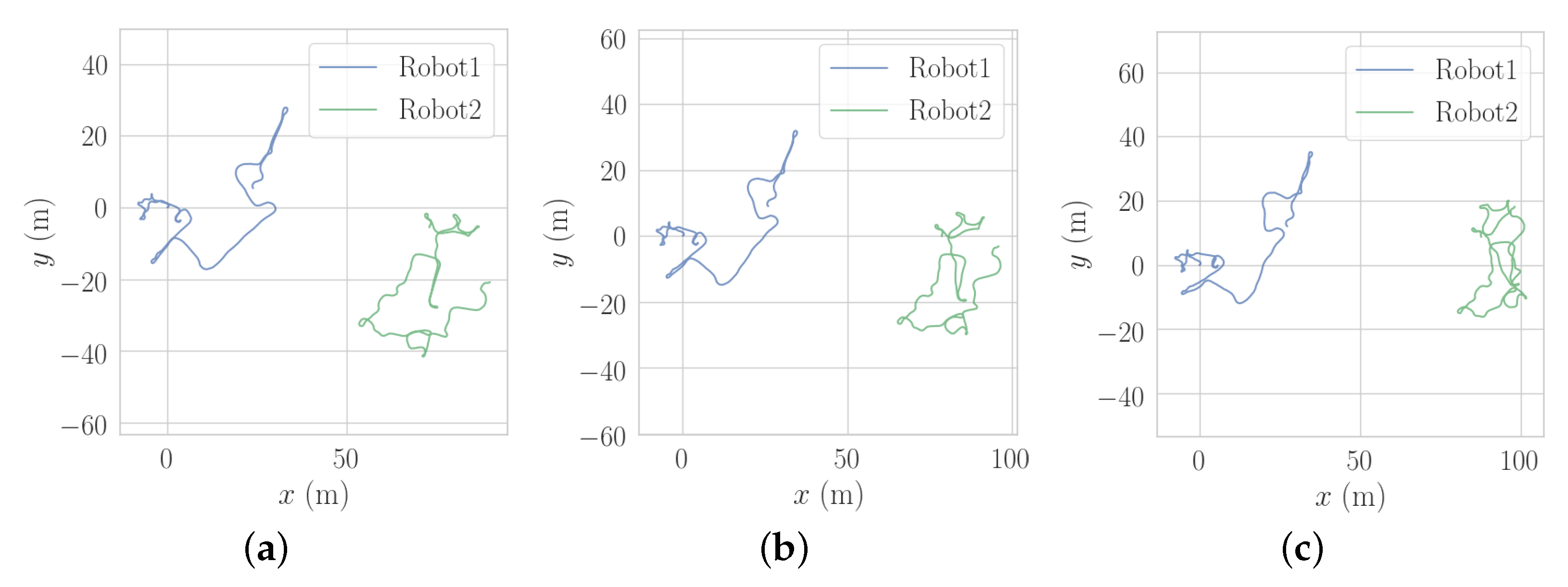
A previous study [4] provided a modified CSAIL dataset that contains two robot trajectories with 128 inlier loop closures and 250 outlier loop closures. In order to compare the robustness of the algorithms to varying odometry error, we added random noise to the orientation of each odometry pose, which affects the overall trajectories cumulatively. Ten noise levels were simulated from 2 σ = 1 to 10 . For each noise level, the noisy trajectories were generated randomly for 100 runs. Figure 7 shows the noisy trajectories at noise levels of 1 , 5 , and 10 , respectively.
We used GTSAM [28] as the framework in our experiments. The baselines are summarized as follows: (1) PCM followed by Gauss–Newton (GN) optimizer with default settings; (2) our initialization technique with PCM followed by default GN optimizer; (3) our initialization technique with DCS solved by default GN optimizer; (4) our initialization technique with our loop closure selection followed by default GN optimizer; (5) D-GNC solved by Levenberg–Marquardt (LM) optimizer with default settings in [6]; (6) our initialization technique with GNC solved by LM optimizer; (7) our initialization technique with our loop closure selection followed by default GN optimizer, where the optimized variable values and the original full pose graph were further optimized by GNC (LM) with identical parameters in baseline (6).
Although PCM does not rely on initialization module to reject outlier measurements, better initial estimates of variable might improve the effect of optimization. Therefore, for comparison, we provide the result of PCM after our initialization as well. DCS turns off all the inter-map factors without initialization [4], and thus, we implement DCS after our initialization. Open source implementations of PCM [29], DCS [30], and D-GNC [29] based on GTSAM are all available online. Parameter sweep was conducted for the following threshold parameters: γ for PCM, Φ for DCS, the inlier threshold for robust distributed PGO in D-GNC, and γ for the proposed loop closure selection method. The best parameters were determined according to the best average Absolute Trajectory Error (ATE) over 100 runs.
Robustness Against Odometry Noise. We compare the performance of concerned algorithms based on Absolute Trajectory Error. Figure 8 shows the distribution of ATE error across 100 runs for each noise level, and quantitative evaluation results for each method against the ground truth are shown in Table A1.
As can be seen, PCM demonstrated great instability (many outliers shown in red plus signs) and the largest errors because of bad initial estimates on the trajectory. Utilizing the proposed initialization with PCM exhibited a positive impact because better initial value estimates improve the effect of the GN optimization. However, the final ATE of PCM, even with our initialization, increased drastically as the noise level increased. Both DCS with our initialization and our proposed method obtained lower ATE and better stability than PCM, and our proposed method performed better when the odometry noise level was greater than 3 . D-GNC demonstrated severe instability caused by inaccurate initialization results, and due to the instability, D-GNC gets higher average ATE than the proposed method. Replacing D-GNC’s initialization module with our initialization technique significantly improved the performance and stability of D-GNC, exhibiting the second-best ATE results. Finally, our proposed method followed by GNC achieved stability and the best overall accuracy.
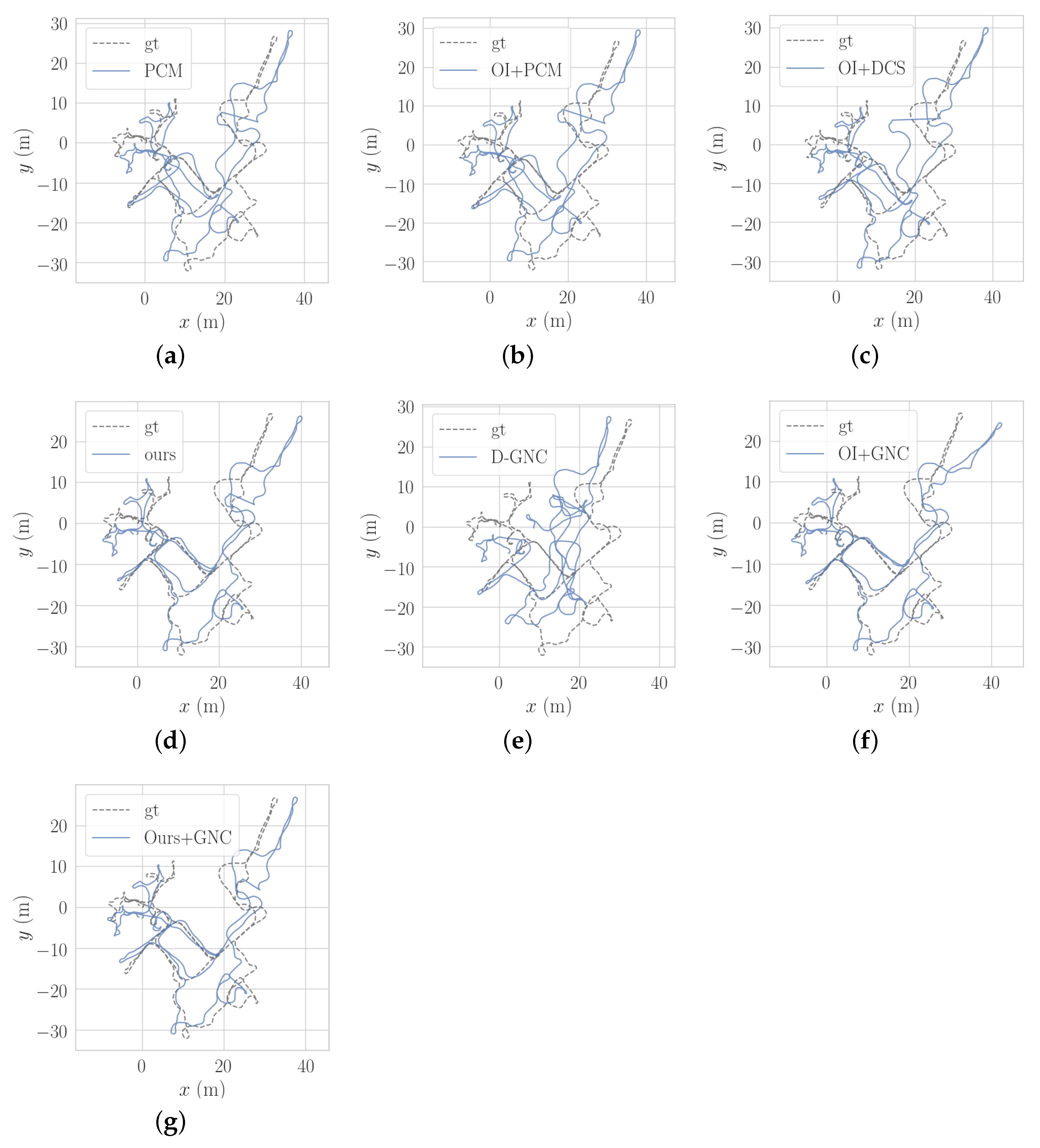
Figure 9 illustrates the trajectory result of different methods on the 39th randomly generated dataset at noise level 8. The obtained trajectory of PCM, PCM with our initialization, DCS with our initialization, and D-GNC exhibit larger drift than our proposed method in most parts of the trajectory. Our proposed method, our initialization with GNC, and our proposed method with GNC show significantly better trajectory results than the four methods mentioned above, especially in the center part of the trajectory. The main difference between these three trajectories is located at the upper-right part of the map, where our proposed method with GNC shows the most similar trajectory to the ground truth, and our initialization with GNC shows the least similar trajectory to the ground truth.
Runtime Comparison. Table 1 shows the average runtimes of the compared methods.
Note that for PCM and our loop closure selection method (O-lcs), the runtime includes the time required to calculate the pairwise consistency metric, MCP or MEWCP, and the GN optimization. As can be seen, DCS outperformed the other methods in terms of runtime efficiency. Our outlier rejection module consumed more time than PCM. The difference is primarily caused by our MEWCP solving time, which is 858 ms on average, compared to PCM’s MCP solving time, which is 175 ms. GNC demonstrated the longest calculation time among all compared methods, and the runtime increases with the noise level. Although D-GNC’s initialization were about one-half that of our initialization technique, this consumed a very small proportion of the procedure’s total runtime. Our initialization technique consumed about 230 to 232 ms, of which 182 milliseconds are used for traversing all the inter-robot loop closure pairs and calculating the c l l ( z i , z j ) (referred to as pairwise-loop consistency) in Equation (11). The rest are used for updating the pose variables of robot trajectories in Equation (12).
Performance of the Proposed Initialization Technique. Table 2 shows the average Absolute Trajectory Errors with different initialization methods.
Here, precision represents the rate at which our proposed initialization method selected a true loop closure as the initial between-robot pose estimate. D-GNC’s initialization obtained much higher ATE than the proposed initialization than ours for two reasons. First, D-GNC’s initialization itself requires a good initial estimate of the relative pose between multiple robots to perform well. Specifically, the robust pose averaging problem in D-GNC’s initialization [6] is formulated as a GNC optimization solved by LM. During this optimization, the pose to be solved is initialized at identity pose, and it has been shown that naive initialization affects the performance of GNC optimizer [6]. In contrast, our initialization does not require this initial estimate. Second, the GNC optimization in D-GNC’s initialization process needs an outlier threshold parameter, which requires an additional parameter tuning to gain robustness against incorrect inter-robot loop closures in actual cases. In contrast, our initialization does not require this additional parameter tuning process.

5.3. Modified Bicocca Dataset

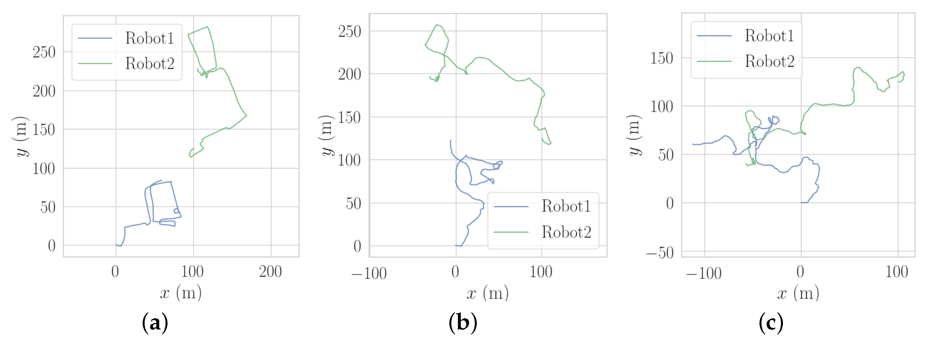
To show the performance of the proposed method on diverse datasets. We also evaluated the performance of our algorithm on a modified Bicocca dataset. The sequence 25b of Bicocca dataset is divided into two robot trajectories. The dataset has 350 loop closures from a simple place recognition algorithm (BoW) with the minimum confidence parameter ( α ) set to 0.15. Among them, 261 loop closures are inliers and the other 89 loop closures are ourliers. Another 172 outlier loop closures were randomly generated as described in the literature [10], in order to increase the outlier rate to 50%. Similarly, we added random noise to the orientation of each odometry pose for ten noise levels from 2 σ = 1 to 10 , in order to simulate scenarios with different odometry errors. For each noise level, 100 noisy trajectories were generated. The implementations and parameter tuning strategies of seven algorithms are the same as those adopted in the modified multi-robot CSAIL dataset. Although modified Bicocca dataset and the modified CSAIL dataset share the similar orientation noise per frame, the trajectory of the Bicocca dataset is much more distorted than that of the CSAIL dataset. Figure 10 shows the noisy trajectories at noise levels of 1 , 5 , and 10 , respectively.
Figure 11 shows the distribution of ATE error across 100 runs for each noise level, and quantitative results for each method against the ground truth is shown in Table A2.
Similar to the CSAIL experiments, the proposed method exhibited greater accuracy and stability over PCM, PCM with our initialization, and D-GNC. Either our initialization or our full method significantly improved the performance and stability of D-GNC, exhibiting the best ATE results.
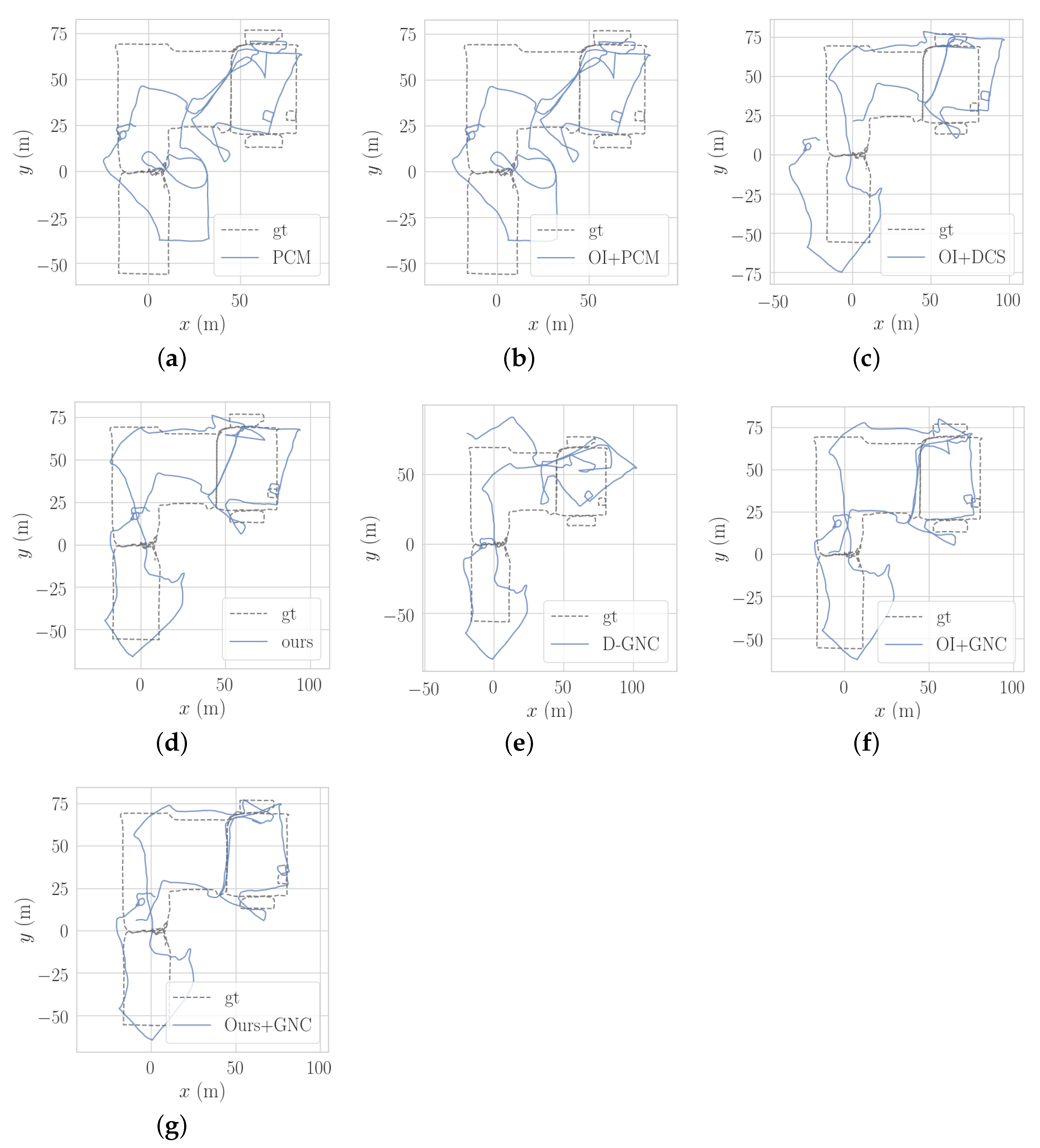
Figure 12 illustrates the trajectory result of different methods on the 28th randomly generated dataset at noise level 3. Similarly, our proposed method, our initialization with GNC, and our proposed method with GNC shows significantly better trajectory results than PCM, PCM with our initialization, DCS with our initialization, and D-GNC. However, the odometry noise exhibits greater impact on Bicocca dataset than CSAIL Dataset. When the odometry noise is larger than 7, the final trajectories provided by all seven methods are hardly applicable. Thus, we try to evaluate the performance of the proposed method from other aspects.
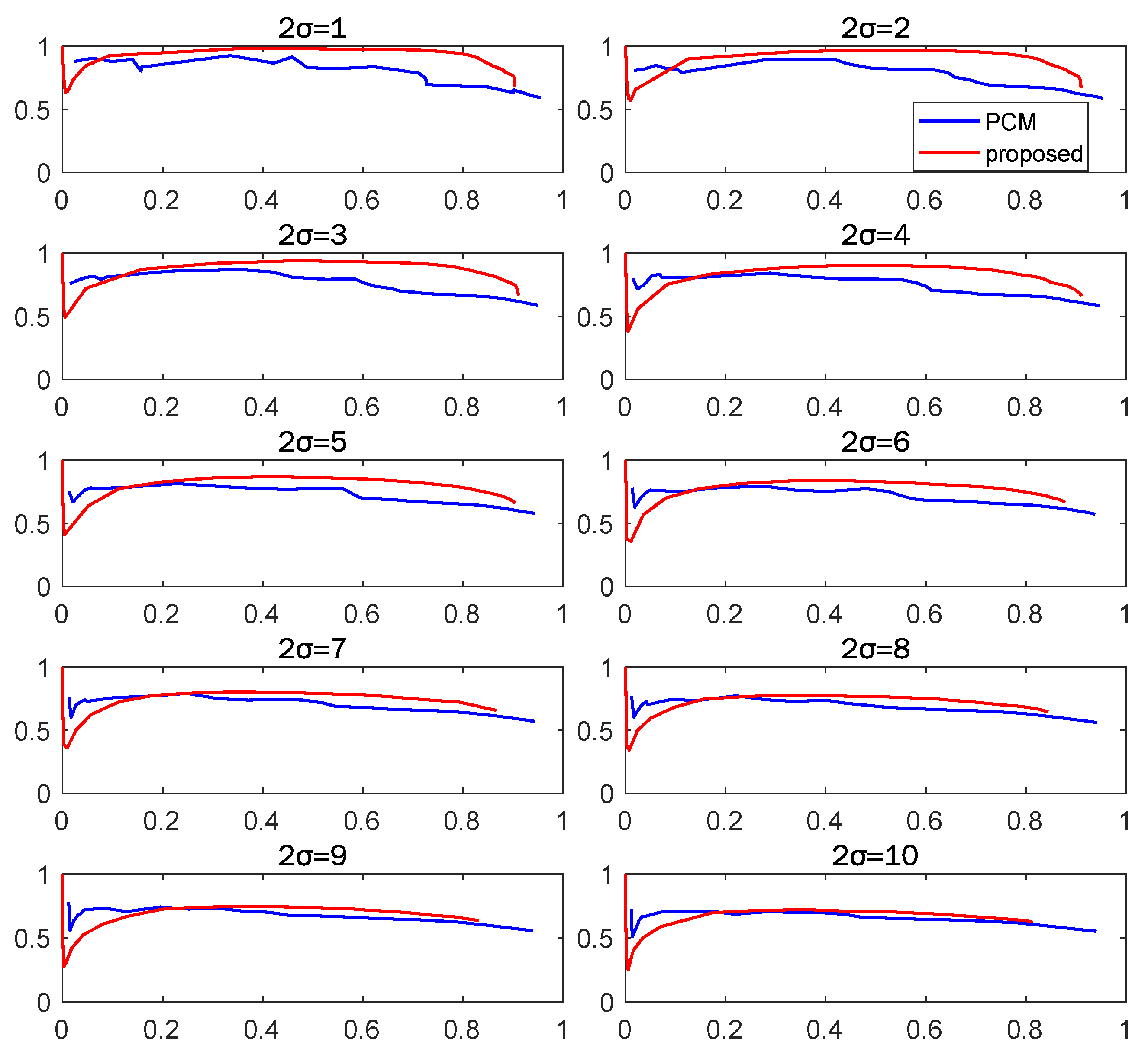
Performance of the Proposed Consistency Metric. Two other important metrics to look at in the context of robust back-ends are precision and recall, especially for outlier rejection methods. An algorithm that provides higher precision with a considerable recall shows better performance. Figure 13 shows the average precision–recall curves of solvers on multi-robot Bicocca dataset under 10 levels of odometry noise.
As can be seen in Figure 13, under low odometry noise, both PCM and our method provide high precision. Under the same recall, PCM gets higher precision only when the recall is lower than 0.2. When recall is higher than 0.2, our proposed method shows higher precision in all of the 10 noise levels. This proves that the proposed method not only provides better final trajectory, but also selects inlier measurements more accuracy than PCM under different odometry noise.

6. Discussion

Evaluation of the Proposed Methods. Our experimental results have proven that the proposed method significantly improves the performance of PCM by a better consistency metric and en extra initialization procedure. Under low odometry error, the proposed method showed slightly better performance than PCM with our initialization, DCS with our initialization, and D-GNC. Under high odometry error, however, the proposed method exhibited significantly better trajectory estimations and stability than PCM with our initialization, DCS with our initialization, and D-GNC. Although GNC with our initialization shows slightly better performance than the proposed method, the runtime of GNC optimization is at least five times longer than our loop closure selection procedure.
Relationship between PCM-like Methods and M-estimation-based Methods. Our experimental results have proven that the proposed method can further improve the performance of GNC [15] by refining pose variable estimates. According to the literature [6], applying GNC after PCM always leads to suboptimal performance due to the low recall of PCM. This low recall is theoretically caused by the formulation of cliques, which finds the best internally consistent measurement rather than all the possible inliers. In other words, the function of PCM-like methods is trusted inlier selection rather than outlier rejection, especially when strict thresholds are applied. Thus, we recommend the usage of PCM-like methods under loose thresholds for updating the pose variable values, followed by M-estimation-based methods, because M-estimation-based methods exhibited better performance when variable values were refined.

7. Conclusions

We proposed a consistency-based inter and intra-robot loop closure selection method for multi-robot map fusion. The proposed method includes an effective initialization strategy that selects a single reliable loop closure as the initial between-robot pose and a modified pairwise consistency metric that serves as weights when we select loop closures with the MEWCP. We compared the proposed method with state-of-the-art robust back-end methods for multi-robot applications. The proposed method shows competitive performance under regular odometry noise, and significantly outperformed the state-of-the-arts methods under severe odometry noise. The proposed consistency metric outperformed PCM under different odometry noise. The proposed initialization method outperformed D-GNC with outliers and noisy odometry, and our loop closure selection method further improved the performance of GNC by providing more accurate variable estimates.

Author Contributions

Conceptualization, J.Z.; methodology, Z.C.; software, Z.C.; validation, Z.C.; formal analysis, Z.C.; investigation, Z.C.; resources, J.Z.; data curation, Z.C.; writing—original draft preparation, Z.C.; writing—review and editing, J.Z.; visualization, Z.C.; supervision, J.Z. and T.F.; project administration, J.Z. and C.Y.; funding acquisition, J.Z. and L.X. All authors have read and agreed to the published version of the manuscript.

Funding

This research was funded by the National Key Research and Development Program of China (No. 2021YFB2501104) and the National Natural Science Foundation of China (No. 41871370).

Data Availability Statement

The ManhattanOlson3500 dataset is available at https://lucacarlone.mit.edu/datasets/ (accessed on 10 May 2023). The multi-robot CSAIL dataset is available at https://github.com/lajoiepy/robust_multirobot_map_merging (accessed on 10 May 2023). The Bicocca dataset is available at https://github.com/ylatif/rrr (accessed on 10 May 2023). The script for generating random loop closures is available at https://github.com/OpenSLAM-org/openslam_vertigo (accessed on 10 May 2023).

Conflicts of Interest

The authors declare no conflict of interest.

Appendix A

Table A1. Average ATE and STD results of the robustly merging map on the multi-robot CSAIL dataset with 10 levels of odometry noise.
Noise Level ( )PCMOI + PCMOI + DCSOursD-GNCOI + GNCOurs + GNC
ATE (m)StdATE (m)StdATE (m)StdATE (m)StdATE (m)StdATE (m)StdATE (m)Std
18.0902.7820.6410.3710.5190.2830.5910.3565.9322.2380.42350.22750.42180.2261
211.8245.7742.0961.2001.8921.0422.0901.1665.5772.2200.84290.45200.84280.4519
315.5027.5124.2052.2854.0272.1773.7532.1045.9282.3071.65100.94771.57590.9139
420.0839.3756.0483.2135.9263.1785.8163.1327.3363.0463.01581.76022.78891.6560
522.49710.3118.3584.4617.6624.0657.2858.5289.2053.9084.52472.60304.52002.6065
625.69211.32010.0925.2949.1584.8928.3489.80511.0384.5776.06053.42205.88963.3359
728.99112.86111.9886.11710.5665.5499.39111.01911.0045.1947.87084.48077.76534.3847
830.76012.69914.0127.06711.5446.05910.06711.82913.2336.2289.07294.99969.03934.9747
934.16114.33215.3647.94612.3426.42610.70512.54915.7287.10410.32455.64259.89865.4318
1035.80214.81517.0038.51813.0646.71011.33413.23317.4777.57111.31576.108811.20586.0329
The best, second-best, and third-best results are highlighted. OI refers to our initialization.
Table A2. Average ATE and STD results of the robustly merging map on the multi-robot Bicocca dataset with 10 levels of odometry noise.
Noise Level ( )PCMOI + PCMOI + DCSOursD-GNCOI + GNCOurs + GNC
ATE (m)StdATE (m)StdATE (m)StdATE (m)StdATE (m)StdATE (m)StdATE (m)Std
1113.95153.98917.6988.25312.3655.15313.4926.09043.33513.8964.02351.85844.21501.8826
2111.40354.10639.96416.65224.66411.70725.57111.95844.85916.98518.93309.314618.94299.3044
3108.03839.65351.49224.93734.98016.51034.29716.15145.27719.41730.370814.768730.302514.7380
498.79538.42162.71530.59640.31518.60738.68217.87346.19220.28336.579417.469836.539717.1571
598.90939.58667.52631.29843.42020.05342.36119.142848.21321.78941.011819.35041.085219.1168
697.37241.46473.04034.73943.63120.19443.23119.563149.36322.46742.322619.818442.467219.924
788.27738.57272.52635.25945.18920.60644.91420.116148.01621.90944.445420.30344.045520.2566
887.08638.35469.03433.88244.55419.71144.29119.26248.61421.77443.652019.194243.363418.9289
977.53234.22368.22532.24644.80019.34144.44318.743447.24121.61643.713818.779244.034118.999
1073.65132.99966.82433.04045.68119.86045.09319.47546.44020.92244.477219.013144.451819.1225
The best, second-best, and third-best results are highlighted. OI refers to our initialization.

References

  1. Wang, X.; Fan, X.; Shi, P.; Ni, J.; Zhou, Z. An Overview of Key SLAM Technologies for Underwater Scenes. Remote Sens. 2023, 15, 2496. [Google Scholar] [CrossRef]
  2. Do, H.; Hong, S.; Kim, J. Robust loop closure method for multi-robot map fusion by integration of consistency and data similarity. IEEE Robot. Autom. Lett. 2020, 5, 5701–5708. [Google Scholar] [CrossRef]
  3. Dellaert, F.; Kaess, M. Factor graphs for robot perception. Found. Trends® Robot. 2017, 6, 1–139. [Google Scholar] [CrossRef]
  4. Mangelson, J.G.; Dominic, D.; Eustice, R.M.; Vasudevan, R. Pairwise consistent measurement set maximization for robust multi-robot map merging. In Proceedings of the 2018 IEEE International Conference on Robotics and Automation (ICRA), Brisbane, QLD, Australia, 21–25 May 2018; pp. 2916–2923. [Google Scholar]
  5. Rosen, D.M.; Doherty, K.J.; Terán Espinoza, A.; Leonard, J.J. Advances in Inference and Representation for Simultaneous Localization and Mapping. Annu. Rev. Control. Robot. Auton. Syst. 2021, 4, 215–242. [Google Scholar] [CrossRef]
  6. Tian, Y.; Chang, Y.; Herrera Arias, F.; Nieto-Granda, C.; How, J.P.; Carlone, L. Kimera-Multi: Robust, Distributed, Dense Metric-Semantic SLAM for Multi-Robot Systems. IEEE Trans. Robot. 2022, 38, 2022–2038. [Google Scholar] [CrossRef]
  7. Fischler, M.A.; Bolles, R.C. Random sample consensus: A paradigm for model fitting with applications to image analysis and automated cartography. Commun. ACM 1981, 24, 381–395. [Google Scholar] [CrossRef]
  8. Latif, Y.; Cadena, C.; Neira, J. Robust loop closing over time for pose graph SLAM. Int. J. Robot. Res. 2013, 32, 1611–1626. [Google Scholar] [CrossRef]
  9. Huber, P.J. Robust estimation of a location parameter. In Breakthroughs in Statistics; Springer: New York, NY, USA, 1992; pp. 492–518. [Google Scholar]
  10. Sünderhauf, N.; Protzel, P. Switchable constraints for robust pose graph SLAM. In Proceedings of the 2012 IEEE/RSJ International Conference on Intelligent Robots and Systems, Vilamoura-Algarve, Portugal, 7–12 October 2012; pp. 1879–1884. [Google Scholar]
  11. Agarwal, P.; Tipaldi, G.D.; Spinello, L.; Stachniss, C.; Burgard, W. Robust map optimization using dynamic covariance scaling. In Proceedings of the 2013 IEEE International Conference on Robotics and Automation, Karlsruhe, Germany, 6–10 May 2013; pp. 62–69. [Google Scholar]
  12. Olson, E.; Agarwal, P. Inference on networks of mixtures for robust robot mapping. Int. J. Robot. Res. 2013, 32, 826–840. [Google Scholar] [CrossRef]
  13. Carlone, L.; Calafiore, G.C. Convex relaxations for pose graph optimization with outliers. IEEE Robot. Autom. Lett. 2018, 3, 1160–1167. [Google Scholar] [CrossRef]
  14. Lajoie, P.Y.; Hu, S.; Beltrame, G.; Carlone, L. Modeling perceptual aliasing in slam via discrete–continuous graphical models. IEEE Robot. Autom. Lett. 2019, 4, 1232–1239. [Google Scholar] [CrossRef]
  15. Yang, H.; Antonante, P.; Tzoumas, V.; Carlone, L. Graduated non-convexity for robust spatial perception: From non-minimal solvers to global outlier rejection. IEEE Robot. Autom. Lett. 2020, 5, 1127–1134. [Google Scholar] [CrossRef]
  16. Dong, J.; Nelson, E.; Indelman, V.; Michael, N.; Dellaert, F. Distributed real-time cooperative localization and mapping using an uncertainty-aware expectation maximization approach. In Proceedings of the 2015 IEEE International Conference on Robotics and Automation (ICRA), Seattle, WA, USA, 26–30 May 2015; pp. 5807–5814. [Google Scholar]
  17. Indelman, V.; Nelson, E.; Dong, J.; Michael, N.; Dellaert, F. Incremental distributed inference from arbitrary poses and unknown data association: Using collaborating robots to establish a common reference. IEEE Control Syst. Mag. 2016, 36, 41–74. [Google Scholar]
  18. Lajoie, P.Y.; Ramtoula, B.; Chang, Y.; Carlone, L.; Beltrame, G. DOOR-SLAM: Distributed, online, and outlier resilient SLAM for robotic teams. IEEE Robot. Autom. Lett. 2020, 5, 1656–1663. [Google Scholar] [CrossRef]
  19. Rosinol, A.; Abate, M.; Chang, Y.; Carlone, L. Kimera: An Open-Source Library for Real-Time Metric-Semantic Localization and Mapping. In Proceedings of the 2020 IEEE International Conference on Robotics and Automation (ICRA), Paris, France, 31 May–31 August 2020; pp. 1689–1696. [Google Scholar]
  20. Ebadi, K.; Chang, Y.; Palieri, M.; Stephens, A.; Hatteland, A.; Heiden, E.; Thakur, A.; Funabiki, N.; Morrell, B.; Wood, S.; et al. LAMP: Large-scale autonomous mapping and positioning for exploration of perceptually-degraded subterranean environments. In Proceedings of the 2020 IEEE International Conference on Robotics and Automation (ICRA), Paris, France, 31 May–31 August 2020; pp. 80–86. [Google Scholar]
  21. Chang, Y.; Tian, Y.; How, J.P.; Carlone, L. Kimera-Multi: A system for distributed multi-robot metric-semantic simultaneous localization and mapping. In Proceedings of the 2021 IEEE International Conference on Robotics and Automation (ICRA), Xi’an, China, 30 May–5 June 2021; pp. 11210–11218. [Google Scholar]
  22. Zheng, S.; Wang, J.; Rizos, C.; Ding, W.; El-Mowafy, A. Simultaneous Localization and Mapping (SLAM) for Autonomous Driving: Concept and Analysis. Remote Sens. 2023, 15, 1156. [Google Scholar] [CrossRef]
  23. Kim, B.; Kaess, M.; Fletcher, L.; Leonard, J.; Bachrach, A.; Roy, N.; Teller, S. Multiple relative pose graphs for robust cooperative mapping. In Proceedings of the 2010 IEEE International Conference on Robotics and Automation, Anchorage, AK, USA, 3–7 May 2010; pp. 3185–3192. [Google Scholar]
  24. Carlone, L.; Censi, A.; Dellaert, F. Selecting good measurements via 1 relaxation: A convex approach for robust estimation over graphs. In Proceedings of the 2014 IEEE/RSJ International Conference on Intelligent Robots and Systems, Chicago, IL, USA, 14–18 September 2014; pp. 2667–2674. [Google Scholar]
  25. Smith, R.; Self, M.; Cheeseman, P. Estimating uncertain spatial relationships in robotics. In Autonomous Robot Vehicles; Springer: New York, NY, USA, 1990; pp. 167–193. [Google Scholar]
  26. Olson, E. Recognizing places using spectrally clustered local matches. Robot. Auton. Syst. 2009, 57, 1157–1172. [Google Scholar] [CrossRef]
  27. Chu, Y.; Liu, B.; Cai, S.; Luo, C.; You, H. An efficient local search algorithm for solving maximum edge weight clique problem in large graphs. J. Comb. Optim. 2020, 39, 933–954. [Google Scholar] [CrossRef]
  28. Dellaert, F. Factor Graphs and GTSAM: A Hands-on Introduction; Georgia Institute of Technology: Atlanta, GA, USA, 2012. [Google Scholar]
  29. MIT-SPARK/Kimera-RPGO: Robust Pose Graph Optimization. Available online: https://github.com/MIT-SPARK/Kimera-RPGO (accessed on 10 May 2023).
  30. Release 4.2a7 · Borglab/Gtsam. Available online: https://github.com/borglab/gtsam/releases/tag/4.2a7 (accessed on 10 May 2023).
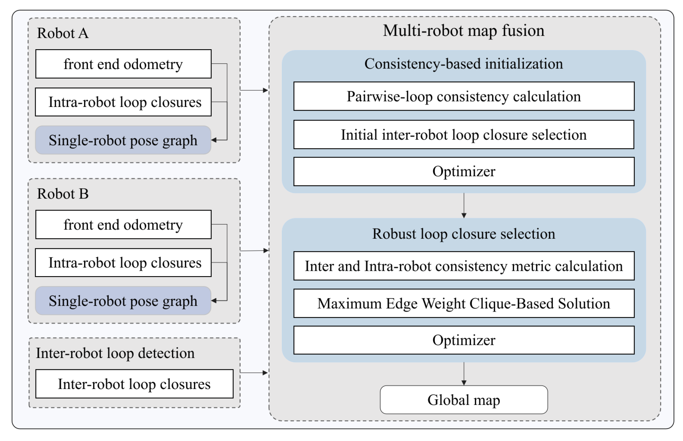
Figure 1. Diagram of the proposed algorithm.
Remotesensing 15 02796 g001
Figure 2. The given pose graph of two robots (blue and orange). Odometry measurements are represented by solid lines. Loop closures are represented by dash lines, inicluding inter-robot loop closures 2, 3, 4 and intra-robot loop closures 1, 5.
Remotesensing 15 02796 g002
Figure 3. The proposed inter and intra-robot consistency metric. (a) Inter-robot loop closure 4 serves as the initial pose between robots in the proposed initialization. (b) The proposed consistency metric between loop 1 and 3; both loop-odometry consistency and pairwise-loop consistency are considered.
Remotesensing 15 02796 g003
Figure 4. The proposed initialization strategy. (a) Using the pairwise-loop consistency, loop closure 4 is selected as a trusted inter-robot loop closure. (b) The selected loop closure serves as the initial pose between robots.
Remotesensing 15 02796 g004
Figure 5. The MEWCP procedure. (a) The value of the proposed metric is stored in a symmetric matrix that can be transformed into a weighted adjacency matrix for a consistency graph. The graph is shown on the top of the matrix. Each node in the graph corresponds to the loop closure of the same color, namely 1 to 5, and each weighted edge denotes the consistency between two measurements. The clique with the largest edge weight (covered by orange shade) corresponds to the most trusted measurement set that fits the internal consistency condition. (b) The best clique can be found by the MEWCP procedure, and the resulting graph can be recovered.
Remotesensing 15 02796 g005
Figure 6. Average precision and recall of MEWCP results with different cutoff times.
Remotesensing 15 02796 g006
Figure 7. (ac) Noisy trajectories of modified CSAIL dataset at noise levels of 1 , 5 , and 10 , sequence 39.
Remotesensing 15 02796 g007
Figure 8. Boxplots of ATE results from 7 solvers on multi-robot CSAIL dataset under 10 levels of odometry noise. Each box shows the ATE for 100 final graphs against the ground truth. The red plus sign demonstrates the outliers, indicating instable results from the solvers.
Remotesensing 15 02796 g008
Figure 9. (ag) Comparison of the map fusion results from different methods on the 39th randomly generated dataset at noise level 8 .
Remotesensing 15 02796 g009
Figure 10. (ac) Noisy trajectories of modified Bicocca dataset at noise levels of 1 , 5 , and 10 .
Remotesensing 15 02796 g010
Figure 11. Boxplots of ATE results results of solvers on multi-robot Bicocca dataset under 10 levels of odometry noise (100 trajectories were generated for each noise level). The red plus sign demonstrates the outliers, indicating instable results from the solvers.
Remotesensing 15 02796 g011
Figure 12. (ag) Comparison of the map fusion results from different methods on the 28th randomly generated dataset at noise level 3 .
Remotesensing 15 02796 g012
Figure 13. Precision–recall curves of solvers on multi-robot Bicocca dataset under 10 levels of odometry noise (100 trajectories were generated for each noise level).
Remotesensing 15 02796 g013
Table 1. Average runtime (ms) of all modules on multi-robot CSAIL dataset.
Noise Level ( )O-iniD-GNC-iniPCMDCSO-lcsGNC
1231811328146217810,897
22321011326103225517,794
3233100134870222418,191
4230101131357224521,279
5232115129956223426,863
6230109129464220225,744
7232117128661224131,033
8231117137653221630,913
9232111140546227127,632
10232107141240223030,652
O-ini refers to our initialization. O-lcs refers to our loop closure selection.
Table 2. Initialization performance on multi-robot CSAIL dataset.
Noise Level ( )D-GNCOurs
ATE (m)StdATE (m)StdPrecision
112.4204.1251.5010.7961.00
210.7083.7723.6341.8581.00
311.1604.1535.3872.7261.00
412.4474.7967.0363.5911.00
513.6865.5258.5564.3581.00
615.1556.0259.8225.0420.98
715.0226.38211.0085.6540.96
816.6317.15911.8386.1280.95
918.9197.91512.6046.4910.93
1020.4228.18113.2676.7630.93
The best results are highlighted.
Disclaimer/Publisher’s Note: The statements, opinions and data contained in all publications are solely those of the individual author(s) and contributor(s) and not of MDPI and/or the editor(s). MDPI and/or the editor(s) disclaim responsibility for any injury to people or property resulting from any ideas, methods, instructions or products referred to in the content.