Article

CSANet: Cross-Scale Axial Attention Network for Road Segmentation

School of Artificial of Intelligence, Xidian University, Xi’an 710071, China
*
Author to whom correspondence should be addressed.
Remote Sens. 2023, 15(1), 3; https://doi.org/10.3390/rs15010003
Submission received: 24 November 2022 / Revised: 14 December 2022 / Accepted: 14 December 2022 / Published: 20 December 2022

Abstract

:
Road segmentation from remote sensing images is an important task in many applications. However, due to the high density of roads and the complex background, the roads are often occluded by trees. This makes accurate road segmentation a challenge task. Most existing road segmentation networks rely on convolutions with small kernels; however, these methods often cannot obtain satisfying results because the long-range dependencies are not captured and the intrinsic relationships between feature maps at different scales are not fully exploited. In this paper, a deep neural network based on a cross-scale axial attention mechanism is proposed to address this problem. This model enables low-resolution features to aggregate global contextual information from high-resolution features. Among them, the axial attention mechanism realizes global attention by using vertical and horizontal attention sequentially. With this strategy, the dense long-range dependencies can be captured with extremely low computational cost. The cross-scale mechanism enables the model to effectively combine the high-resolution fine-grained features and the low-resolution coarse-grained features. The proposed method enables the network to propagate the information without losing details. Our method achieves IoUs of 58.98 and 65.28 on the Massachusetts Roads dataset and DeepGlobe dataset and outperforms other methods.

Graphical Abstract

1. Introduction

Semantic segmentation is a very important and challenging task in the field of computer vision. It has very important applications in many scenarios such as autonomous driving, indoor navigation, and virtual and augmented reality [1,2]. Road segmentation is one of the basic tasks of aerial imagery processing, which aims to separate pixels belonging to roads from other background pixels in remote sensing aerial images. Road segmentation plays an essential role in many applications, such as traffic management, emergency tasks, road monitoring, etc.
Compared with conventional semantic segmentation, road segmentation in aerial images relies more on global contextual information because the shape of roads is usually long and continuous. Early road-segmentation methods were mostly implemented with complex hand-crafted features, such as the morphology-based method proposed by Steger et al. [3] and the texture analysis and beam transform-based method proposed by Sghaier et al. [4]. The methods based on topology improve the accuracy by post-processing the segmentation map, but this undoubtedly brings a higher computational cost [5,6,7]. With the rapid development of deep learning, convolutional neural networks are well known for their end-to-end properties and powerful feature-modeling capabilities. It is also widely used in road image segmentation. The split depth-wise separable Graph-Convolution Network proposed by Zhou et al. [8] separates spatial features and channel features with depth-wise separable convolutions, and then the Sobel gradient operator is used to construct the adjacency matrix of the feature map to extract the road information. Lan et al. [9] introduce residual dilated convolution and ASPP modules on the basis of Unet to expand the receptive field and capture multi-scale global context information. Tao et al. [10] designed a spatial information inference structure that enables multidirectional message passing between pixels. It is thus possible to learn local visual features of roads and global spatial structure information (such as road continuity and trend). Henry et al. [11] introduce the sensitivity of the spatial tolerance rule to thin objects so that most of the roads in the test set can be identified. Shamsolmoali et al. [12] apply structured domain adaptation to synthetic image generation and road segmentation, in which a feature pyramid (FP) network is incorporated into a generative adversarial network to minimize the difference between the source and target domains. Y-Net [13] extracts features through a downsampling-to-upsampling sub-network and a sub-network without downsampling. Then, the features of these two parts are combined by the fusion module for road segmentation. However, fully convolutional networks can only capture local information through their small convolution kernels, while for long-range dependencies, they are obtained by stacking these convolution kernels. Due to the inductive bias of the fully convolutional network itself, capturing long-range dependencies requires passing through multiple deep network layers. This results in low computational efficiency, and the network is difficult to optimize. For example, when the information of two feature points in the feature map needs to be transferred to each other, it will be very difficult. Yu et al. [14] proposed dilation convolution to dilate the receptive field. Although dilation convolution can expand the receptive field while reducing the number of feature map by downsampling, for road segmentation, it can only obtain information from very limited surrounding feature points and cannot obtain long-range context awareness. Conditional random fields (CRFs) [15], which model long-range dependencies, are used to post-process predictions for semantic segmentation. However, doing so brings additional computational overhead.
Some methods in the field of natural language processing have been applied to semantic segmentation and achieved very good results, such as the self-attention-based method [16]. It calculates the response of a position by the weighted sum of the similarity of all positions in the sequence. The non-local attention is also introduced for semantic segmentation in a similar way [17]. Although long-range dependencies can be captured with these methods, the non-local network needs to generate huge attention maps. This leads to a huge time and space complexity of O ( N 2 ) , as shown in Figure 1a. N refers to the total number of spatial feature points within the feature map.
For cross-scale feature aggregation, most of the existing deep-neural-network-based methods sample features of different scales to a uniform size and then combine them by pixel-wise summation or concatenation. We believe that such an aggregation method will lose some details due to the information loss in the up- and down-sampling process.
In order to simultaneously capture the global information of features and efficiently combine the information between different scales, a cross-scale axial attention-based method is proposed in this paper. To reduce the large computational cost in non-local networks, the axial attention mechanism is adopted. Specifically, we first compute the attention map on the vertical axis, followed by the attention map on the horizontal axis. Finally, the network aggregates two feature maps with different spatial resolution sizes in a non-local manner. With the proposed method, each element in the low-resolution feature map contains the global information of the high-resolution feature map, as shown in Figure 1b. We validated our model on the Massachusetts Roads dataset [18] and DeepGlobe dataset [19]. Overall, this paper makes the following contributions:
  • A novel deep model is proposed for road segmentation, which adopts a global attention mechanism to exploit the long dependence.
  • Our proposed method is able to capture dense contextual information and better combine features at different scales. This results in more accurate road segmentation results.
  • The proposed method consumes less computing resources than most other networks.

2. Related Work

2.1. None-Local Network

Non-local networks borrowed ideas from the self-attention mechanism proposed in the field of natural language processing, which has also achieved good results in the field of computer vision [20,21]. Non-local networks are designed to build global relationships [22]. Specifically, each feature point in the feature map is composed of the weighted sum of all the feature points in the whole image. Feature points with higher similarity to this point will have higher weights and vice versa. The non-local neural network was first proposed by Wang et al. [17], inspired by non-local means to construct an operator that can capture long-distance dependencies. DANet [23] constructs a dual attention network to aggregate long-range dependencies in spatial and channel dimensions, respectively. PSANet [24] builds global dependencies by learning adaptive attention masks and designing bidirectional information-propagation paths. OCNet [25] defines pixels of the same class as each other’s target semantics and constructs an attention map by calculating the dependency between each pixel in the feature map and its corresponding target semantics. DFN [26] uses the channel attention mechanism to distinguish feature channels of different importance during the upsampling process to solve the problem of intra-class inconsistency and adds boundary constraints to increase the difference between different classes. GCNet [27] finds that the global context information obtained by different query positions through the non-local structure is almost the same. Therefore, in order to reduce unnecessary computation, a simplified non-local structure is proposed. Chi et al. [28] propose a learnable and data-adaptive bilinear attention transform (BA-Transform). A wide range of local and global attention operations can be modeled in a data-adaptive manner. Different attention operations are often applied to different feature channel groups to resolve the differences between features. Yin et al. [29] decoupled the non-local term into a pairwise term and a unary term and make them independent of each other in learning content and gradient propagation to achieve better performance.

2.2. Axial Attention

Although non-local structures can coordinate global context information, the high computational complexity makes the model very cumbersome and difficult to train. In order to solve this problem, a new axial-recurrent attention mechanism emerges. Specifically, each element in the feature map only performs self-attention to the row and column alternately. At the same time, each element in the feature map can spread the attention range from one row or one column to the whole image with circular axial attention. Axial-DeepLab [30] proposes a position-sensitive axial attention model, in which noteworthy remote dependencies can be precisely captured. CCNet [31] obtains the attention map by paying attention to the contextual information of the cross paths where its pixels are located. By incorporating channel axial attention in calculating the spatial axial attention map, CA [32] greatly relieves the conflict between the previous channel attention and the spatial attention and improves the performance. NN-UNet [33] captures 3D features by using axial attention on the horizontal, vertical, and channel axes of the feature map in the decoder part. Medical Transformer [34] proposes a gated axial attention model, which extends existing architectures by introducing additional control mechanisms in the self-attention module. Furthermore, it operates on whole images and patches to learn global and local features, respectively. CaraNet [35] proposes a context-axis-preserving attention method to improve the segmentation performance for small objects.

3. Method

3.1. Overall Network Framework

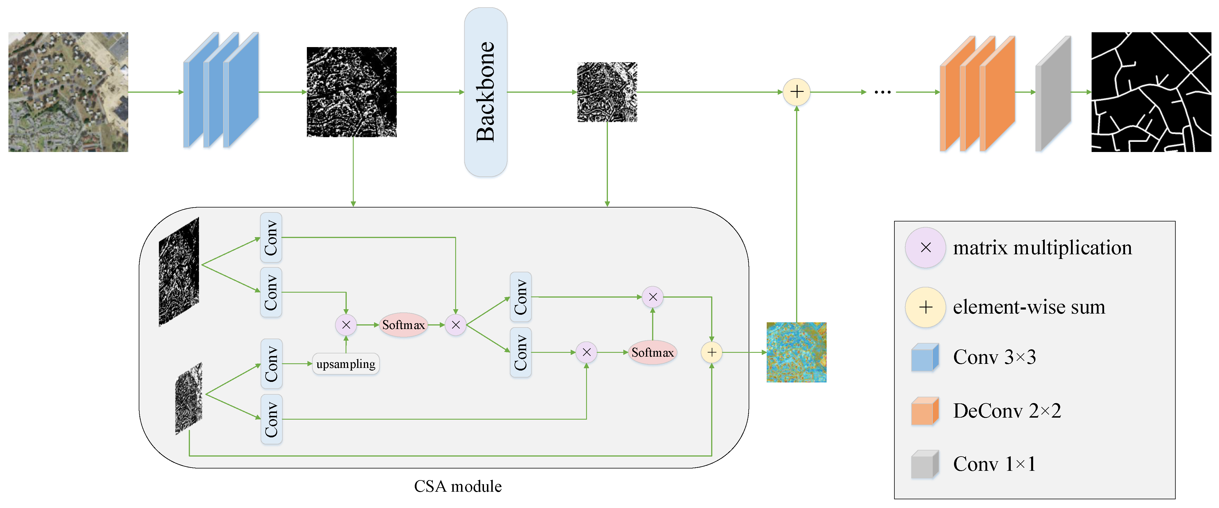
The overall architecture of our proposed model is shown in Figure 2. It consists of an initialization layer, a backbone network (CFPNet [36]), the Cross-Scale Axial Attention (CSA) module, and an upsampling layer. The CSA module can combine global attention across different scales during the propagation process. Specifically, the initialization layer initializes the input image as the input features through three consecutive convolution operations and downsamples the length and width to 1/2 of the original size for subsequent computations. Our network backbone is mainly composed of CFP modules [36]. This module captures multi-scale contextual information in the form of parallel stacked asymmetric convolutions. In the process of forward propagation, the feature resolution is reduced layer by layer to capture global information. The CSA module performs information fusion on feature maps of two different scales. Among them, high-resolution features contain more detailed information and local features, while low-resolution features contain more global features, but some details will inevitably be lost. Dense context awareness is captured by continuous vertical and horizontal attention from high-resolution features to low-resolution features. The obtained attention map is added to the original feature map so that the network backbone can capture dense long-range dependencies without losing detailed information during the propagation process. In the upsampling part, we use the deconvolution operation instead of conventional bilinear interpolation to restore the features to the input size layer by layer and output the final road segmentation result. Although this will slightly increase the network parameters, convolutional learning can learn a better fitting method than manual design.

3.2. Backbone

In order to obtain higher performance and reduce the computation burden as much as possible, we adopt the CFP module proposed by Lou et al. [36] as the backbone of the proposed method. In this paper, we stack multiple CFP modules into two CFP clusters. They are called CFP-1 and CFP-2, respectively. As the features pass through these two clusters, the resolution is downsampled to 1/4 and 1/8 of the original image, respectively. CFP-1 consists of CFP modules with expansion ratios of [2, 2]. CFP-2 consists of CFP modules with expansion ratios of [4, 4, 8, 8, 16, 16]. The CFP module is defined as follows:
y i = j = 1 i f W i n x , r j
z = W o u t y 1 , y 2 , y 3 , y 4 + x
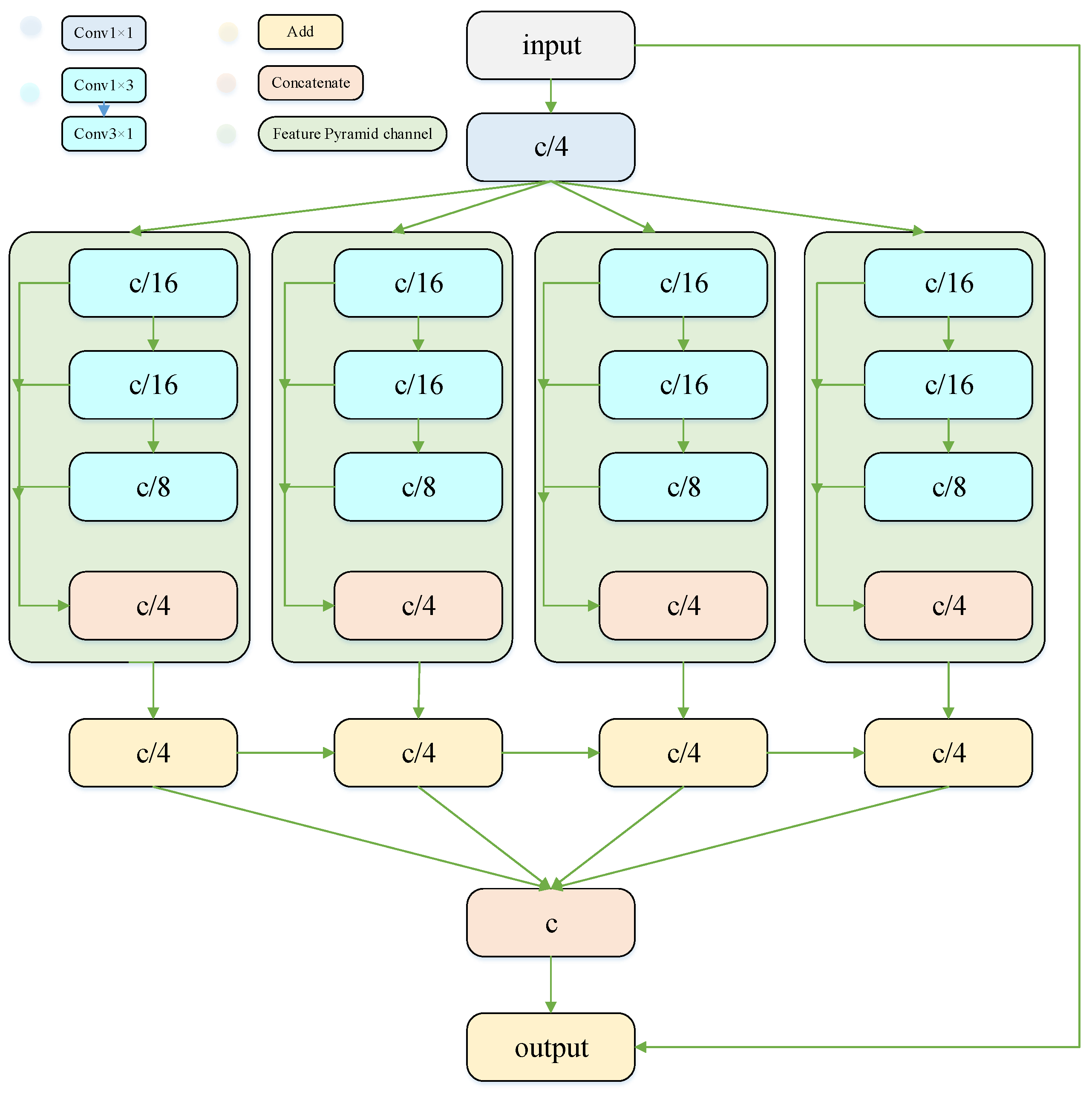
where x is the input feature of the CFP module. We assume that the number of channels of x is C. Both W i n and W o u t are a 1 × 1 convolution. r j is the dilation rate of the jth feature pyramid channel. f represents the mapping function of the feature pyramid channel. [ · , · ] is the concatenation operation. We first reduce the input dimension from C to C/4 by passing x through W i n . The features are then sent to four feature pyramid channel modules with different dilation rates. As shown in the green part of Figure 3, their expansion rates are r 1 = 1 , r 2 = d / 4 + 1 , r 3 = d / 2 + 1 , and r 4 = d + 1 . d is the dilation ratio for the CFP module. Then, we start with the feature map of the second feature pyramid channel and add this feature to the previous features to obtain the final 4 multi-scale feature maps of dimension C/4, that is, y 1 , y 2 , y 3 , y 4 . Finally, we concatenate these four feature maps together to obtain feature maps of the same dimension as the input, and activate them via W o u t . To prevent the introduction of asymmetric convolutions to make the network deeper and harder to train, we add the input feature x to the output using residual connections [21]. The overall structure of the CFP module is shown in Figure 3.
For the feature pyramid channel, we borrow the idea of inception [37,38,39,40]. We replace the 5 × 5 and 7 × 7 convolution kernels with two and three pairs of asymmetric convolutions, respectively. Furthermore, the number of filters of the first to third pairs of asymmetric convolutions is set to C/16, C/16, and C/8, respectively. In this way, multi-scale feature maps with different receptive fields can be constructed with less computational overhead. In order to further reduce the amount of calculation, we share the convolution kernel and extract features from each pair of asymmetric convolutions and then concatenate them together. Finally, a multi-scale feature map with dimension C/4 is obtained. The calculation process of the feature pyramid channel can be expressed as follows:
x i = w r x i 1
f ( x , r ) = x 1 , x 2 , x 3
where w r represents a pair of asymmetric convolutions with dilation rate r. x 0 is the input feature and [ · , · ] is the concatenatin operation.

3.3. CSANet

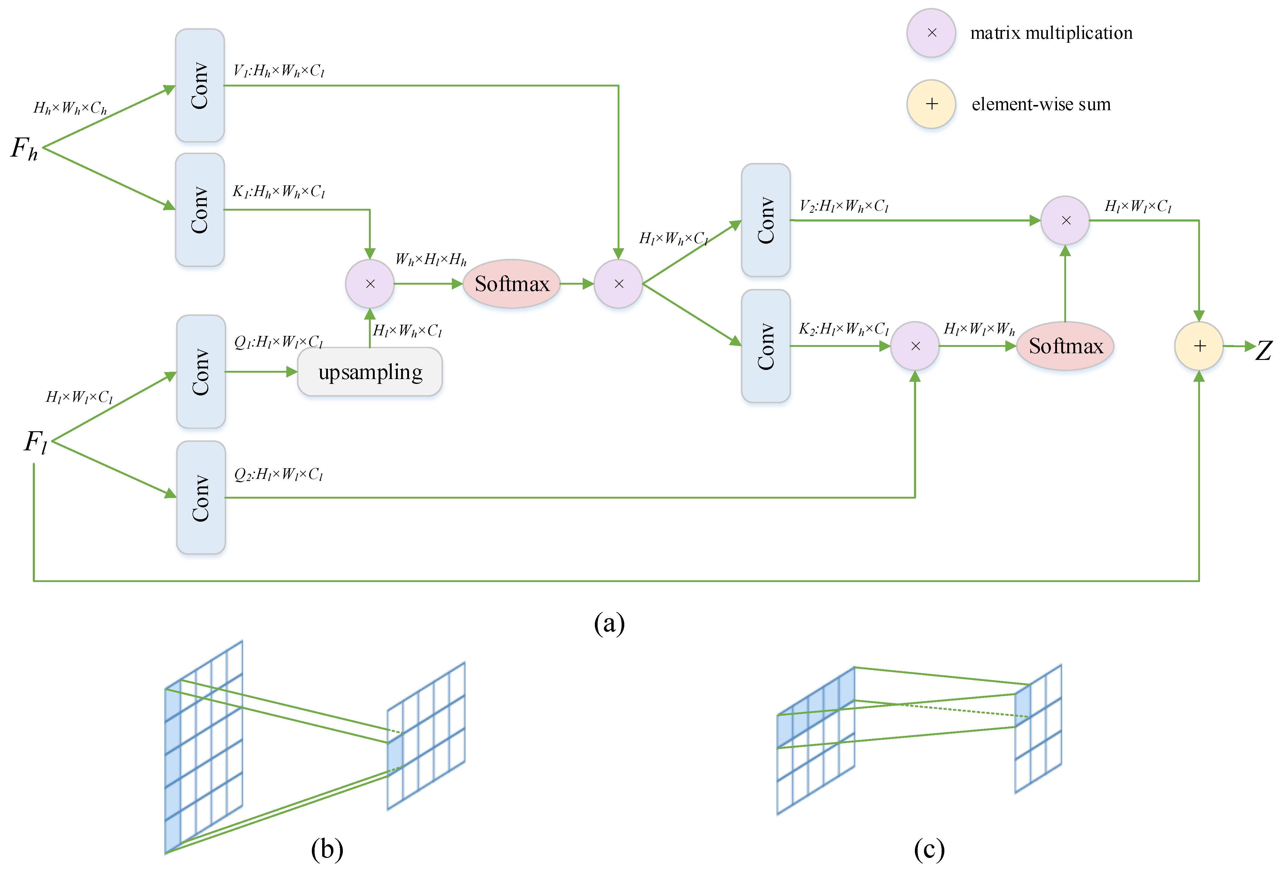
A schematic diagram of the CSA module is shown in Figure 4. Current multi-scale backbone architectures only use simple concatenation and summation when integrating information between scales. In this process, the information interaction between different scales is not exploited. The information contained in the feature maps of different scales has a different emphasis. Among them, the high-resolution feature maps contain more position and detail information such as texture, geometry, and contour. The low-resolution feature map contains more abstract semantic information, which is a grasp of the image as a whole. The effective fusion of features of different scales can effectively reduce the information loss in the process of forward propagation. Furthermore, for the topological dependence of the road segmentation problem, it is crucial to establish long-range dependencies. The CSA module addresses both issues simultaneously by generating attention maps for low-resolution features and high-resolution features. In this paper, we have established two CSA modules called CSA-1 and CSA-2. Among them, CSA-1 acts on the high-resolution features after the initialization layer and the medium-resolution features after CFP-1. CSA-2 acts on updated medium-resolution features of CSA-1 and the low-resolution features of CFP-2. Specifically, given a high-resolution feature F h R W h × H h × C h and a low-resolution feature F l R W l × H l × C l , similar to self-attention, F l obtains the query vector Q 1 R W l × H l × C l through a 1 × 1 convolution. F h is mapped to the key vector K 1 R W h × H h × C l and the value vector V 1 R W h × H h × C l through two 1 × 1 convolutions. To align the channel dimensions for computing the attention map, we map the channel dimensions from C h to C l when computing K and V. Next, we put axial attention to the longitudinal axis of these two features. To align their widths, we upsample the horizontal axis of Q 1 from W l to W h by asymmetric deconvolution and obtain an updated Q 1 R W h × H l × C l . Q 1 and K 1 are then multiplied and normalized by softmax to obtain the similarity matrix S 1 R W h × H l × H h . Specifically, we obtain the similarity matrix as follows:
S 1 x h , y l , y h = e Q 1 x h , y l × K 1 x h , y h y = 1 H h e Q 1 x h , y l × K 1 x h , y
Any element x h , y l , y h in S 1 represents the similarity between the element x h , y l in F 2 and x h , y h in F 1 . Then, multiplication of S 1 and V 1 is performed to obtain the column-dependent attention feature map M 1 R W h × H l × C l of F 2 for F 1 . The specific calculation process of M 1 is expressed as
M 1 x h , y l = y = 1 H h S 1 x h , y l , y × V 1 x h , y
At this point, each element in F 2 is composed of the weighted sum of the corresponding columns in F 1 ; that is, each element in F 2 contains the entire column context information of the corresponding column in F 1 .
To enable F 2 to obtain global contextual information about F 1 , we calculate the vertical axis attention map based on the horizontal axis attention map. We map F 2 to a query vector Q 2 R W l × H l × C l through a convolution of 1 × 1 and pass M 1 through two 1 × 1 convolutional layers to obtain K 2 , V 2 R W h × H l × C l . Then, a similar operation on the horizontal axis can be performed as the vertical axis. The similarity matrix S 2 R W h × W l × H l is obtained by multiplying Q 2 and K 2 and going through softmax. The calculation process of S 2 is as follows:
S 2 y l , x l , x h = e Q 2 x l , y l × K 2 x h , y l x = 1 W h e Q 2 x l , y l × K 2 x , y l
Wherein any point y l , x l , x h in S 2 represents the similarity between the element x l , y l in F 2 and the element x h , y l in M 1 . Finally, we multiply S 2 and V 2 to obtain the global attention feature map M 2 R W l × H l × C l of F 2 for F 1 . The calculation process of M 2 is as follows:
M 2 x l , y l = x = 1 W h S 2 y l , x l , x × V 2 x , y l
Since we perform the axial attention of the vertical axis initially, each element of F 2 contains the context information of the corresponding column of F 1 , as shown in Figure 4b. We then perform axial attention on the horizontal axis, as shown in Figure 4c. Therefore, each element contains contextual information of the entire row and each element in a row contains contextual information of an entire column. In this way, each element contains global contextual information. At the same time, compared with the non-local calculation method shown in Figure 1b, time and space complexity is reduced from O ( n × N ) to O n N ( N + n ) , where n and N represent the total number of elements in the F 2 and F 1 along spatial dimensions, respectively.
The proposed method captures and combines dense contextual information across scales through axial attention. Compared to convolutional networks, we have a larger receptive field and denser context awareness. Each feature point in the feature map is related to the entire feature map. This is critical for extremely topological targets such as roads. It can ensure that a connection can be established between any two points on a long and narrow road, rather than only relying on local features. For example, for roads covered by trees, we can combine distant road features to make predictions without the limitation that convolutional networks can only extract local features. Compared to non-local networks, our model has fewer parameters and requires less computation. By stacking axial attention, we reduce the computational burden effectively without losing accuracy. Additionally, our method combines information across different scales more effectively. Each element in the low-resolution feature is obtained by weighting and summation of the high-resolution features. Thus, the information loss during the downsampling process of the image is reduced.

4. Experiments

4.1. Datasets

4.1.1. Massachusetts Roads Dataset

The Massachusetts Roads dataset is provided from V. Mnih’s doctoral dissertation [18]. It is a high-quality aerial road imagery dataset, which includes urban, suburban, rural, and other areas in Massachusetts. The total sampling area is over 2600 square kilometers. The size of each image is 1500 × 1500, and the spatial resolution is 1 m. Its training and test sets contain 1108 and 63 images, respectively. We split the image into small images at equal intervals in order to use a larger batch size to improve training effectiveness. We first upsampled the training set to 1536 × 1536 size by bilinear interpolation and crop them to small images of size 512 × 512 with a stride of 256. In this way, each training image is cropped to obtain 25 small images. At the same time, the occluded images were removed from the dataset to avoid negatively impacting the network training. For the test sets, we crop them into small images of 512 × 512 with a stride of 512. This leaves no overlapping area between each two small cropped images. Each image is divided into nine small images. Finally, the training set and test set consist of 21,951 and 567 images, respectively. The dataset is available from https://www.cs.toronto.edu/~vmnih/data/ (accessed on 23 November 2022).

4.1.2. DeepGlobe Dataset

This dataset is presented by the deepglobe2018 challenge. The data cover urban and rural areas in India, Indonesia, and Thailand. The DeepGlobe dataset contains 6226 images with ground truth. The size of each image is 1024 × 1024, and each pixel contains an area of two square meters. We use 4696 of them as the training set and the remaining 1530 as the test set. Similarly, we divide the training set into 9 512 × 512 small images with stride of 256, and divide the test set into 512 × 512 small images with stride 512. In the end, we obtained 42,264 images as the training set and 6120 images as the test set. The dataset is available at https://competitions.codalab.org/competitions/18467 (accessed on 23 November 2022).

4.2. Implementation Details

All our experiments adopted the following settings. We used two RTX 3090 GPUs to train the model under the framework of pytorch. Only simple random rotation and random flip were used for data augmentation. The optimizer for training the network was Adam, and the initial learning rate was set to 0.001. We updated the learning rate using a step-learning scheduler with an interval of 30. The learning rate was reduced to 0.1 times the original for each update. The loss function was a binary cross-entropy loss. The batchsize was set to 16, and the model was trained for a total of 100 epochs.

4.3. Metrics

Since the road width in the ground truth of Massachusetts is consistent, it does not match the real scene. Therefore, we used relaxed IoU (IoU r ) to evaluate the results [41]. The relaxation factor is 4. The Precision, Recall, IoU, Accuracy and F1 score were also used to evaluate the model’s performance.

5. Results

5.1. Comparison with Other Classic Methods

In this section, we quantitatively and qualitatively compare the proposed method with other classic methods. Next, we briefly introduce the comparison methods.
1.
UNet [42]: This method adopts an encoder–decoder structure and captures local information through small convolution kernels. In the decoder part, the corresponding encoder features and decoder features are concatenated and the resolution is gradually recovered through a deconvolution operation.
2.
SegNet [43]: SegNet captures local information by stacking convolutional layers, and a lot of convolution operations and unpooling are used to restore the resolution in the decoder part.
3.
PSPNet [44]: The PSPNet method is based on multiscale feature fusion and introduces more contextual features through a global mean pooling operation. It downsamples features to different scales and reduces the feature dimension through 1 × 1 convolutional layers.
4.
ENet [45]: ENet increases the receptive field by atrous convolution and reduces information loss effectively by combining downsampling and pooling.
5.
DeepLabv3 [46]: This method captures multiscale information with parallel atrous convolution at different sampling rates through the Atrous Spatial Pyramid Pooling (ASPP) module.
6.
CFPNet [36]: CFPNet expands the receptive field with a small number of parameters through parallel asymmetric atrous convolution.

5.2. Segmentation Results on Massachusetts Roads Dataset

The quantitative results for the Massachusetts Roads dataset are summarized in Table 1. All the evaluation metrics of methods such as UNet and SegNet that capture local information by stacking convolution kernels are lower than the proposed CSANet. This shows that the long-range dependence in road segmentation is difficult to accomplish through the network structure in the form of stacked convolution kernels.
All evaluation metrics of PSPNet except IoU r are lower than the proposed method. We argue that simply concatenating features at different scales together cannot capture their intrinsic connections. However, our CSANet captures their connections through dense attention operations between scales, resulting in more accurate segmentation results.
Atrous convolution-based methods such as ENet, DeepLabv3, and CFPNet can expand the receptive field and reduce the parameters by downsampling. The performance of ENet is lower than the proposed CSANet in all metrics except Precision. All metrics of DeepLabv3 are lower than the CSANet. All metrics of CFPNet except IoU r are lower than those of our method. These methods fail to capture dense contextual information. However, our CSANet can capture dense contextual information through a cross-scale axial attention mechanism. Overall, for the Massachusetts Roads dataset, the proposed method achieves the best performance on Recall, IoU, Accuracy, and F1. This shows that our proposed CSANet can capture global context information and exploit more information by cross-scale fusion.
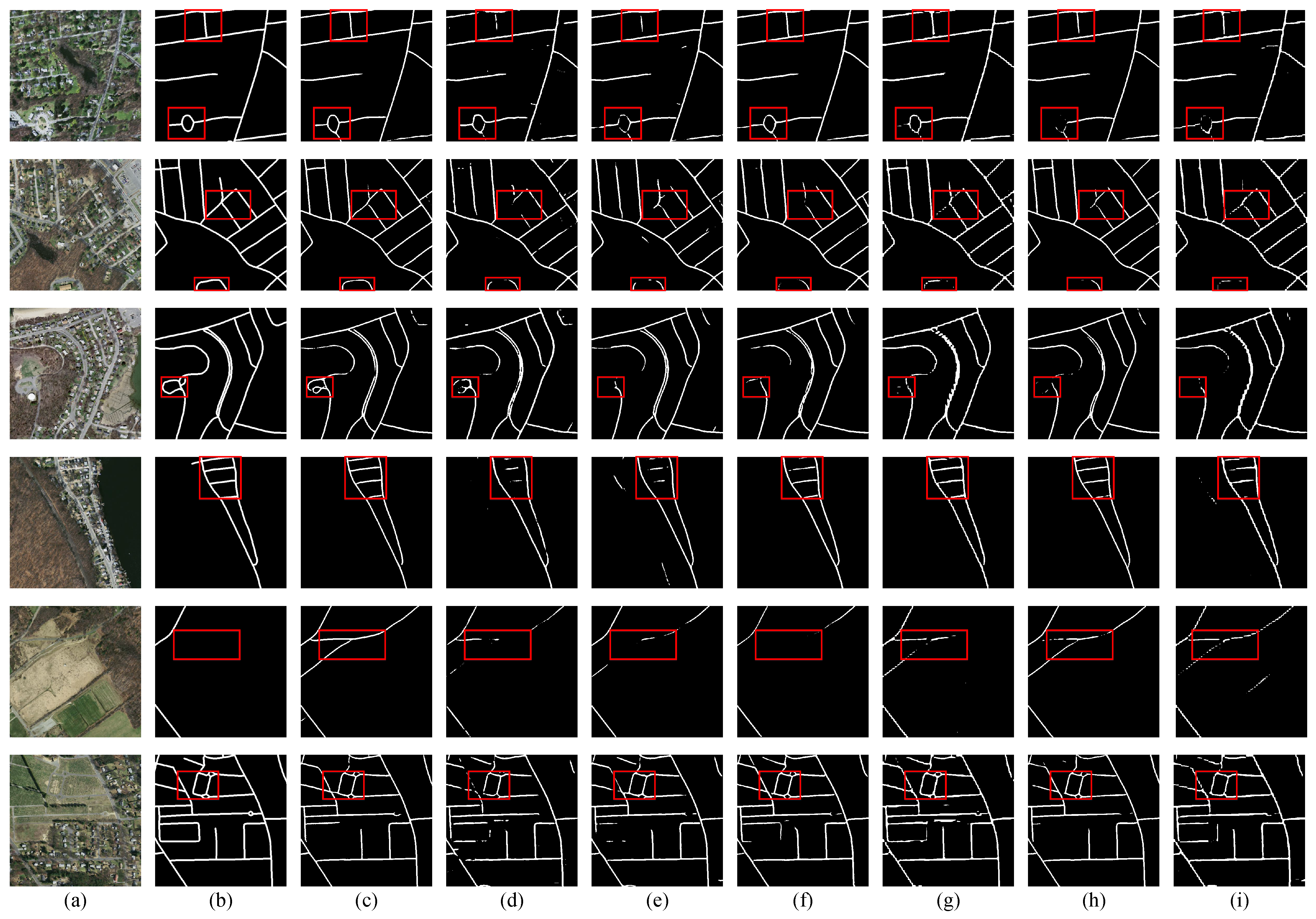
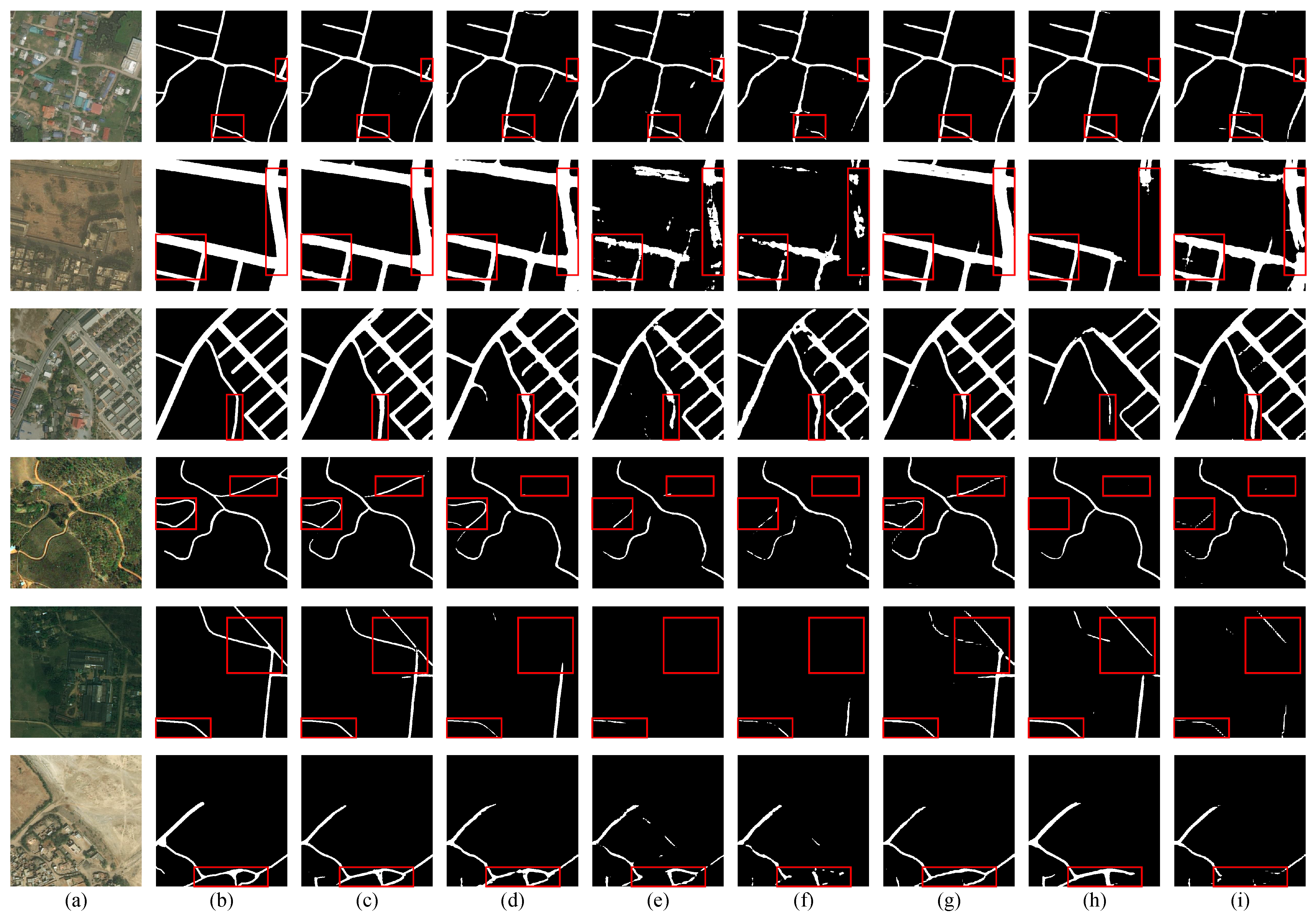
For qualitative analysis, we present the segmentation results of the proposed CSANet with UNet, ENet, DeepLabv3, CFPNet, SegNet, and PSPNet of the Massachusetts Roads dataset. As shown in Figure 5, the red boxes highlight the most obvious differences between different methods. In the small-town road scene in the second row of Figure 5, some parts of large area of the road are blocked by trees. UNet, SegNet, PSPNet, and atrous convolution-based networks all fail to segment roads correctly, whereas the proposed CSANet infers the correct result by the correlation of this location with all other locations.
Overall, all methods can segment most of the roads successfully. However, the segmentation results of comparison methods have breakpoints or noise in some complex road segments. This shows that traditional convolutional networks cannot extract long-distance information of roads due to the limited receptive field of small convolution kernels. It can only identify whether a pixel block belongs to a road by some road features. This leads to the incoherent and false detection of roads. Our proposed CSANet is able to extract both global and cross-scale information. The fusion of multi-scale features is more conducive to the network to grasp the integrity and continuity of the road.

5.3. Segmentation Results on DeepGlobe Dataset

The quantitative results for the DeepGlobe dataset are shown in Table 2. For the DeepGlobe dataset, the conclusions are generally consistent with those of the Massachusetts Roads dataset. However, the Accuracy of UNet is slightly higher than that of our method. This is due to its strong robustness that results in improved background segmentation. Furthermore, the Precision metric of ENet is lower than that of the proposed method. The IoU r of DeepLabv3 is lower than thta of the proposed method. This shows that the proposed CSANet can generalize to other types of data without degrading the segmentation accuracy. For the DeepGlobe dataset, the CSANet achieved the best performance on Precision, IoU, IoU r , and F1.
The visual segmentation results of the DeepGlobe dataset are shown in Figure 6. For the forest road scene in the fourth row of Figure 6, the small road in the red box at the upper right is difficult to identify because it is too narrow and blocked by trees. The proposed CSANet is able to aggregate global information across scales. Thus, details are not lost during downsampling, and the road can be segmented correctly.

5.4. Segmentation Maps

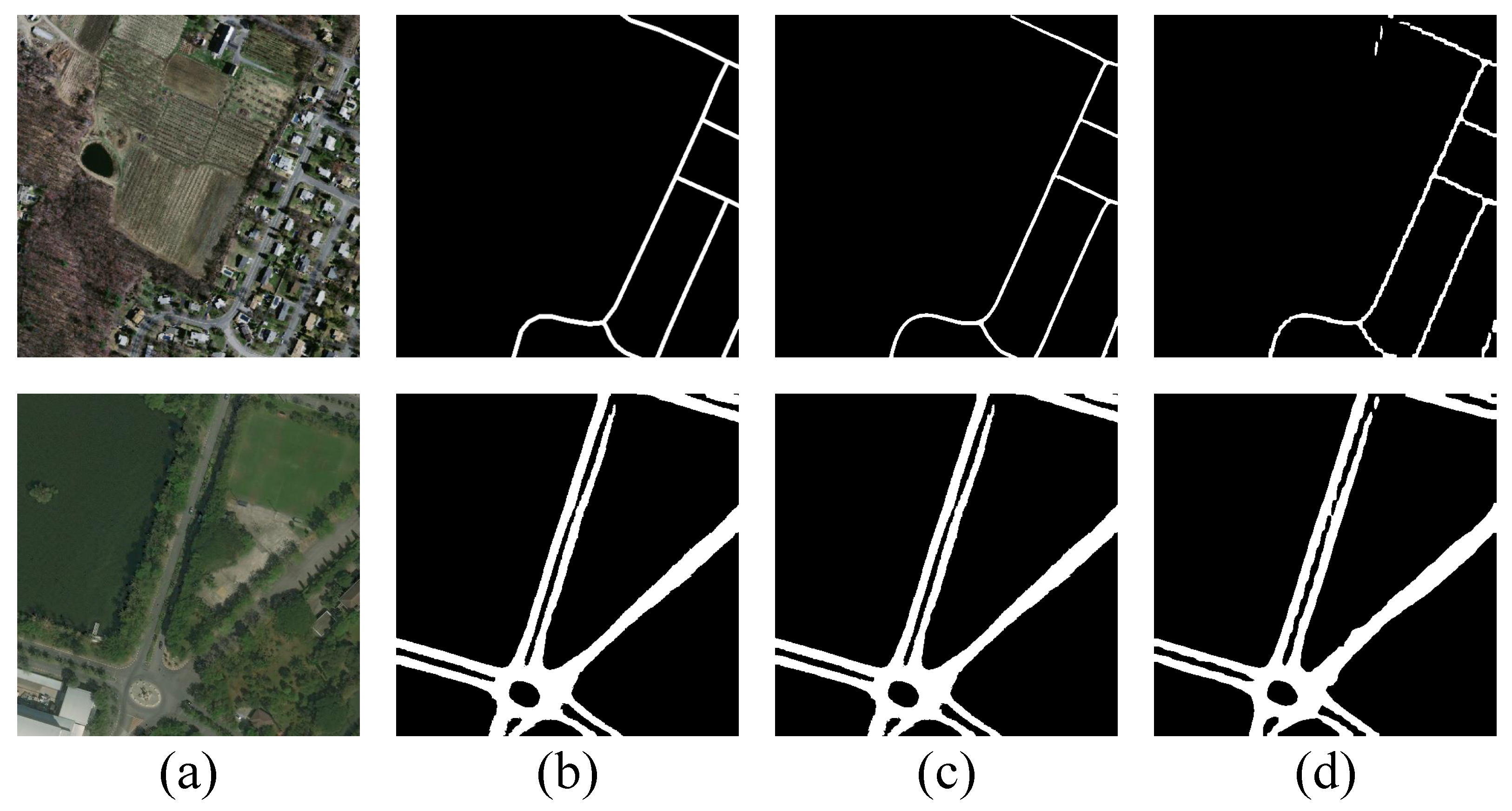
Figure 7 shows the segmentation visualization results of our proposed CSANet and CFPNet. It can be seen that CFPNet has obvious jagged lines on the edge of the road (it is best to zoom in on the picture to view). In contrast, the segmentation results of our method have smooth edges and natural transitions. This shows that our method is able to capture dense contextual information. Furthermore, our proposed attention-based cross-scale information fusion method can make the high-level features in the deep layers of the network not lose the details in the shallow layers. Although CFPNet captures global information through the channel feature pyramid, the limitation of the size of the convolution kernel causes it to only capture long-range discrete information. Our method not only achieves optimal performance on evaluation metrics but also performs well on actual segmentation maps.

5.5. Ablation Studies

An ablation study is performed to verify the effectiveness of the CSA module. Table 3 and Table 4 show the quantitative results on the Massachusetts Roads dataset and the DeepGlobe dataset, respectively. The baseline (No. 1) is the network built with the CFP module. No. 2 and No. 3 indicate that the CSA-1 module and CSA-2 module are added to the baseline, respectively. The results show that both CSA-1 and CSA-2 can improve the baseline network. Compared with CSA-2, CSA-1 improves the network performance more significantly. The CSA-1 module acts on the high-resolution feature maps of the first downsampling and the medium-resolution feature maps of the second downsampling. Similarly, the CSA-2 module acts on medium-resolution feature maps and low-resolution feature maps. This shows that our CSA module is more effective in the initial stage of network propagation, i.e., when the size of the feature maps is large. No. 4 means that both the CSA-1 module and the CSA-2 module are introduced. At this point, the network achieves the highest performance. The above results show that our method is able to combine high-resolution and low-resolution information effectively.
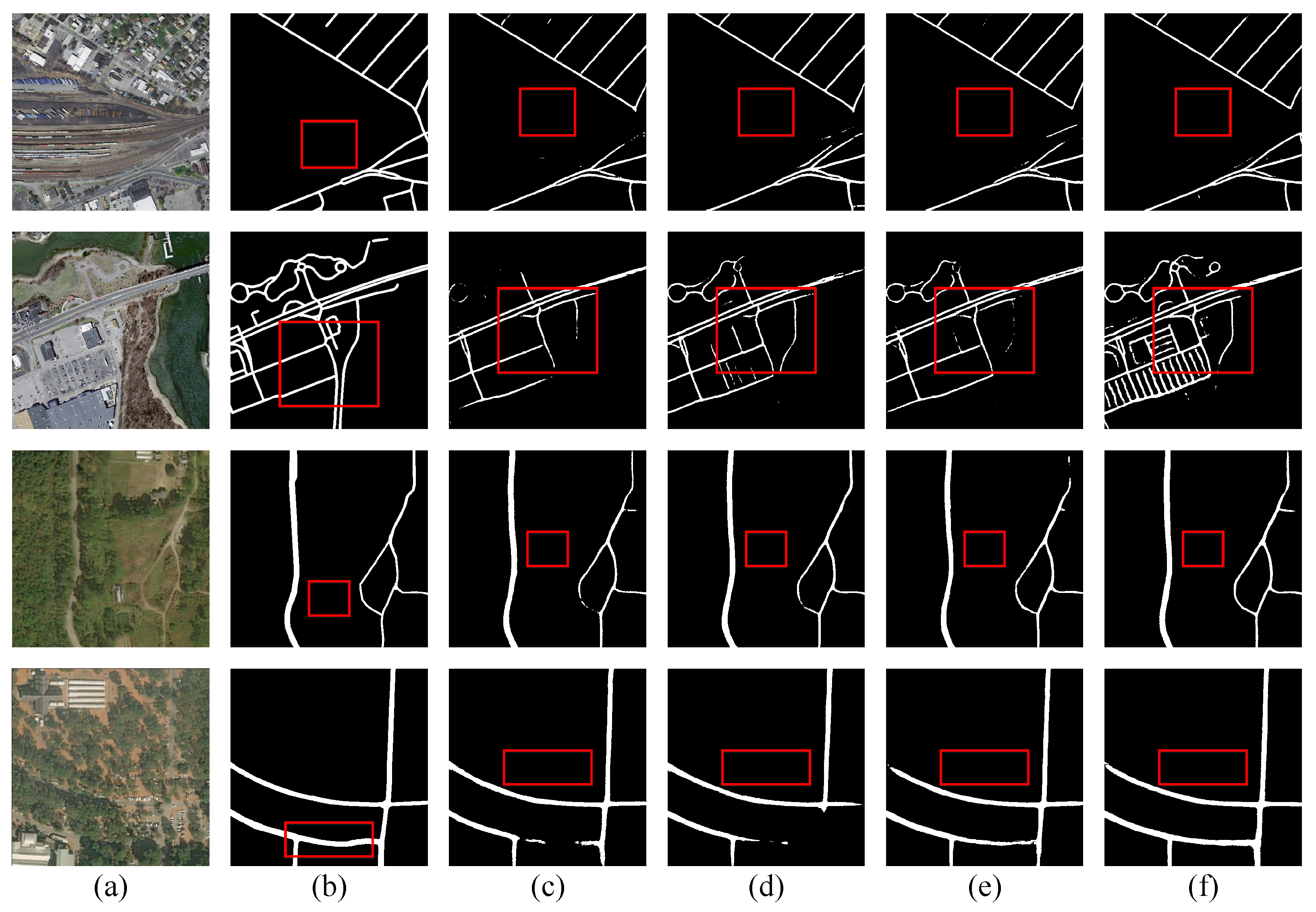
Figure 8 shows the qualitative results on the Massachusetts Roads dataset and the DeepGlobe dataset. The red box is used to highlight the difference between different segmentation models. In the second row of Figure 8, for the parking lot scene of the Massachusetts Roads dataset, our CSANet (No. 4) recognized the interior narrow passages of parking lots that were not marked in the ground truth. In contrast, No. 1 did not recognize the inner passage of the parking lot at all. No. 2 only identified some road debris. No. 3 identified a few internal passages of the parking lot. With the introduction of CSA-1 and CSA-2, the proposed method could capture and combine both high-level and low-level semantics information effectively. As a result, details that could be captured by the baseline network (No. 1) were identified. In the fourth row of Figure 8, in the highway scene of the DeepGlobe dataset, due to the occlusion of trees and shadows on both sides of the road, the pixels of the road within this range were different from other parts, which made the road difficult distinguish. Networks No. 1 and No. 2 were barely able to identify the segment. With the support of CSA-1, No. 3 successfully captured the high-level semantic features of the road section and gave the correct segmentation results. Likewise, Network No. 4 gave a more complete segmentation map with the help of CSA-1 and CSA-2. The above qualitative results demonstrate the effectiveness of the proposed CSA module.

5.6. Computational Complexity Analysis

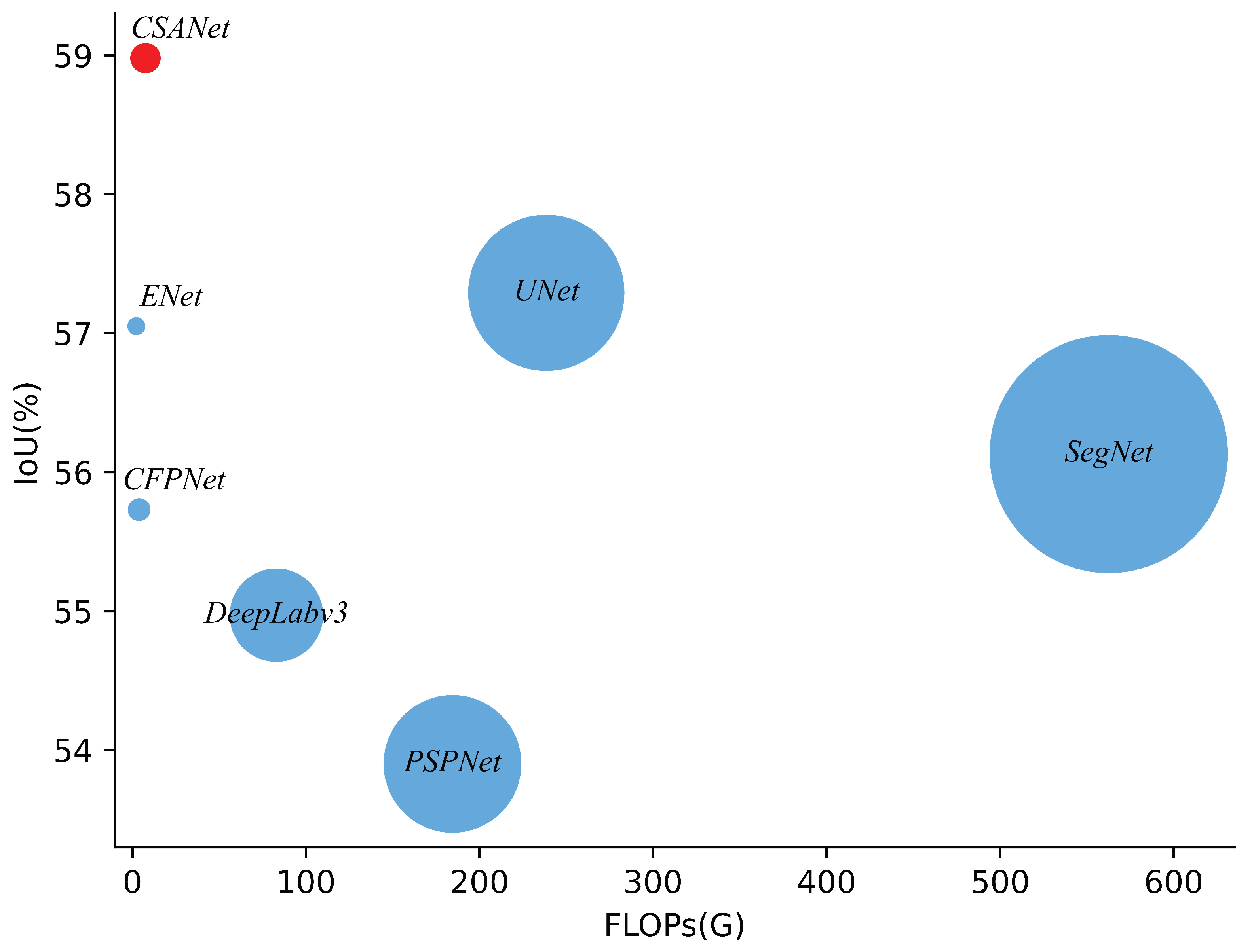
Table 5 summarizes the computational cost of different methods and their IoU accuracy on the Massachusetts Roads dataset. The proposed CSANet achieves the best performance with a relative small number of parameters and computation burden.
Figure 9 visually shows the relationship between the computation burden and the IoU accuracy on the Massachusetts Roads dataset. The area of a circle is proportional to the computational complexity. ENet has a small computational load due to its use of small convolution kernels throughout the process. CFPNet and CSANet greatly reduce the amount of computation by introducing depth-wise separable convolutions. Furthermore, our CSANet uses axial attention to compute the attention map. Therefore, the computation burden is reduced further. DeepLabv3 also uses depth-wise separable convolution in Xception, so it has a smaller amount of computation. SegNet has a huge computation complexity because it has a large number of convolution operations in the encoding and decoding parts.
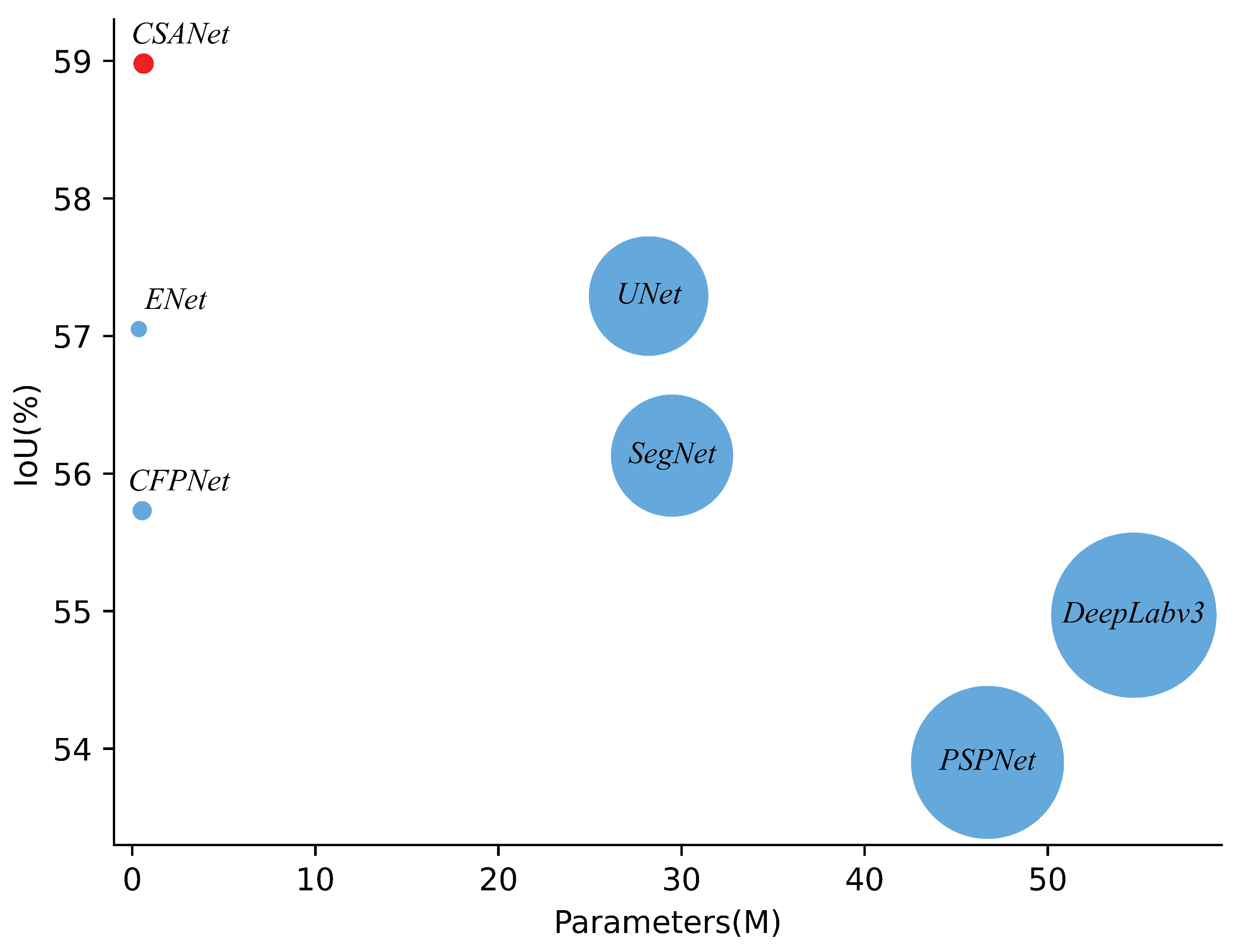
Figure 10 visually shows the relationship between the parameter size and the IoU accuracy on the Massachusetts Roads dataset. The area of each circle is proportional to its parameter amount. UNet brings more parameters due to its wide network structure (the number of channels increases exponentially during downsampling). The SegNet uses a large number of convolution operations in the encoding and decoding part, which also brings more parameters. PSPNet has a large number of parameters because it aggregates features at multiple scales. Furthermore, due to the existence of the ASPP module in DeepLabv3, the computation of multiscale, features with different receptive fields brings additional parameters. ENet uses asymmetric convolution to reduce the number of parameters and atrous convolution to expand the receptive field. CFPNet reduces the number of parameters by stacking parallel asymmetric depthwise convolutions. The CSANet also uses asymmetric convolution to reduce the parameter size. The CSANet achieves state-of-the-art performance with a comparable number of parameters to lightweight networks such as ENet and CFPNet.

6. Conclusions

In this paper, a novel cross-scale axial attention network is proposed. This method can exploit the high-resolution fine-grained information and low-resolution coarse-grained information with a layer-by-layer mechanism, and axial attention is introduced to extract the global contextual information. This enables the proposed method to produce road segmentation maps with higher integrity and continuity. The evaluation results based on the Massachusetts Roads dataset and DeepGlobe dataset validate the fact that our method outperforms classic segmentation algorithms.

Author Contributions

Conceptualization, X.C. and K.Z.; methodology, X.C.; software, K.Z.; validation, K.Z.; formal analysis, L.J.; investigation, X.C.; resources, K.Z.; data curation, K.Z.; writing—original draft preparation, K.Z. and writing—review and editing, X.C., K.Z. and L.J. All authors have read and agreed to the published version of the manuscript.

Funding

This work was supported by the National Natural Science Foundation of China (No.62176199 and 61805189).

Data Availability Statement

Not applicable.

Conflicts of Interest

The authors declare no conflict of interest.

References

  1. Xu, Z.; Sun, Y.; Liu, M. icurb: Imitation learning-based detection of road curbs using aerial images for autonomous driving. IEEE Robot. Autom. Lett. 2021, 6, 1097–1104. [Google Scholar] [CrossRef]
  2. Xu, Z.; Sun, Y.; Liu, M. Topo-boundary: A benchmark dataset on topological road-boundary detection using aerial images for autonomous driving. IEEE Robot. Autom. Lett. 2021, 6, 7248–7255. [Google Scholar] [CrossRef]
  3. Steger, C.; Glock, C.; Eckstein, W.; Mayer, H.; Radig, B. Model-based road extraction from images. In Automatic Extraction of Man-Made Objects from Aerial and Space Images; Springer: Berlin/Heidelberg, Germany, 1995; pp. 275–284. [Google Scholar]
  4. Sghaier, M.O.; Lepage, R. Road extraction from very high resolution remote sensing optical images based on texture analysis and beamlet transform. IEEE J. Sel. Top. Appl. Earth Obs. Remote Sens. 2015, 9, 1946–1958. [Google Scholar] [CrossRef]
  5. Máttyus, G.; Luo, W.; Urtasun, R. Deeproadmapper: Extracting road topology from aerial images. In Proceedings of the IEEE International Conference on Computer Vision, Venice, Italy, 22–29 October 2017; pp. 3438–3446. [Google Scholar]
  6. Batra, A.; Singh, S.; Pang, G.; Basu, S.; Jawahar, C.; Paluri, M. Improved road connectivity by joint learning of orientation and segmentation. In Proceedings of the IEEE/CVF Conference on Computer Vision and Pattern Recognition, Long Beach, CA, USA, 16–17 June 2019; pp. 10385–10393. [Google Scholar]
  7. Mosinska, A.; Marquez-Neila, P.; Koziński, M.; Fua, P. Beyond the pixel-wise loss for topology-aware delineation. In Proceedings of the IEEE Conference on Computer Vision and Pattern Recognition, Salt Lake City, UT, USA, 18–23 June 2018; pp. 3136–3145. [Google Scholar]
  8. Zhou, G.; Chen, W.; Gui, Q.; Li, X.; Wang, L. Split Depth-wise Separable Graph-Convolution Network for Road Extraction in Complex Environments from High-resolution Remote-Sensing Images. IEEE Trans. Geosci. Remote Sens. 2021, 60, 5614115. [Google Scholar] [CrossRef]
  9. Lan, M.; Zhang, Y.; Zhang, L.; Du, B. Global context based automatic road segmentation via dilated convolutional neural network. Inf. Sci. 2020, 535, 156–171. [Google Scholar] [CrossRef]
  10. Tao, C.; Qi, J.; Li, Y.; Wang, H.; Li, H. Spatial information inference net: Road extraction using road-specific contextual information. ISPRS J. Photogramm. Remote Sens. 2019, 158, 155–166. [Google Scholar] [CrossRef]
  11. Henry, C.; Azimi, S.M.; Merkle, N. Road segmentation in SAR satellite images with deep fully convolutional neural networks. IEEE Geosci. Remote Sens. Lett. 2018, 15, 1867–1871. [Google Scholar] [CrossRef] [Green Version]
  12. Shamsolmoali, P.; Zareapoor, M.; Zhou, H.; Wang, R.; Yang, J. Road segmentation for remote sensing images using adversarial spatial pyramid networks. IEEE Trans. Geosci. Remote Sens. 2020, 59, 4673–4688. [Google Scholar] [CrossRef]
  13. Li, Y.; Xu, L.; Rao, J.; Guo, L.; Yan, Z.; Jin, S. A Y-Net deep learning method for road segmentation using high-resolution visible remote sensing images. Remote Sens. Lett. 2019, 10, 381–390. [Google Scholar] [CrossRef]
  14. Yu, F.; Koltun, V. Multi-scale context aggregation by dilated convolutions. arXiv 2015, arXiv:1511.07122. [Google Scholar]
  15. Wegner, J.D.; Montoya-Zegarra, J.A.; Schindler, K. A higher-order CRF model for road network extraction. In Proceedings of the IEEE Conference on Computer Vision and Pattern Recognition, Portland, OR, USA, 23–28 June 2013; pp. 1698–1705. [Google Scholar]
  16. Vaswani, A.; Shazeer, N.; Parmar, N.; Uszkoreit, J.; Jones, L.; Gomez, A.N.; Kaiser, Ł.; Polosukhin, I. Attention is all you need. Adv. Neural Inf. Process. Syst. 2017, 30, 1–11. [Google Scholar]
  17. Wang, X.; Girshick, R.; Gupta, A.; He, K. Non-local neural networks. In Proceedings of the IEEE Conference on Computer Vision and Pattern Recognition, Salt Lake City, UT, USA, 18–23 June 2018; pp. 7794–7803. [Google Scholar]
  18. Mnih, V. Machine Learning for Aerial Image Labeling; University of Toronto: Toronto, ON, Canada, 2013. [Google Scholar]
  19. Demir, I.; Koperski, K.; Lindenbaum, D.; Pang, G.; Huang, J.; Basu, S.; Hughes, F.; Tuia, D.; Raskar, R. Deepglobe 2018: A challenge to parse the earth through satellite images. In Proceedings of the IEEE Conference on Computer Vision and Pattern Recognition Workshops, Salt Lake City, UT, USA, 18–22 June 2018; pp. 172–181. [Google Scholar]
  20. Hou, S.; Shi, H.; Cao, X.; Zhang, X.; Jiao, L. Hyperspectral Imagery Classification Based on Contrastive Learning. IEEE Trans. Geosci. Remote Sens. 2021, 60, 5521213. [Google Scholar] [CrossRef]
  21. He, K.; Zhang, X.; Ren, S.; Sun, J. Deep residual learning for image recognition. In Proceedings of the IEEE Conference on Computer Vision and Pattern Recognition, Las Vegas, NV, USA, 27–30 June 2016; pp. 770–778. [Google Scholar]
  22. Wang, L.; Li, R.; Zhang, C.; Fang, S.; Duan, C.; Meng, X.; Atkinson, P.M. UNetFormer: A UNet-like transformer for efficient semantic segmentation of remote sensing urban scene imagery. ISPRS J. Photogramm. Remote Sens. 2022, 190, 196–214. [Google Scholar] [CrossRef]
  23. Fu, J.; Liu, J.; Tian, H.; Li, Y.; Bao, Y.; Fang, Z.; Lu, H. Dual attention network for scene segmentation. In Proceedings of the IEEE/CVF Conference on Computer Vision and Pattern Recognition, Long Beach, CA, USA, 15–20 June 2019; pp. 3146–3154. [Google Scholar]
  24. Zhao, H.; Zhang, Y.; Liu, S.; Shi, J.; Loy, C.C.; Lin, D.; Jia, J. Psanet: Point-wise spatial attention network for scene parsing. In Proceedings of the European Conference on Computer Vision (ECCV), Munich, Germany, 8–14 September 2018; pp. 267–283. [Google Scholar]
  25. Yuan, Y.; Huang, L.; Guo, J.; Zhang, C.; Chen, X.; Wang, J. Ocnet: Object context network for scene parsing. arXiv 2018, arXiv:1809.00916. [Google Scholar]
  26. Yu, C.; Wang, J.; Peng, C.; Gao, C.; Yu, G.; Sang, N. Learning a discriminative feature network for semantic segmentation. In Proceedings of the IEEE Conference on Computer Vision and Pattern Recognition, Salt Lake City, UT, USA, 18–23 June 2018; pp. 1857–1866. [Google Scholar]
  27. Cao, Y.; Xu, J.; Lin, S.; Wei, F.; Hu, H. Gcnet: Non-local networks meet squeeze-excitation networks and beyond. In Proceedings of the IEEE/CVF International Conference on Computer Vision Workshops, Seoul, Korea, 27–28 October 2019. [Google Scholar]
  28. Chi, L.; Yuan, Z.; Mu, Y.; Wang, C. Non-local neural networks with grouped bilinear attentional transforms. In Proceedings of the IEEE/CVF Conference on Computer Vision and Pattern Recognition, Seattle, WA, USA, 13–19 June 2020; pp. 11804–11813. [Google Scholar]
  29. Yin, M.; Yao, Z.; Cao, Y.; Li, X.; Zhang, Z.; Lin, S.; Hu, H. Disentangled non-local neural networks. In Proceedings of the European Conference on Computer Vision, Glasgow, UK, 23–28 August 2020; Springer: Berlin/Heidelberg, Germany, 2020; pp. 191–207. [Google Scholar]
  30. Wang, H.; Zhu, Y.; Green, B.; Adam, H.; Yuille, A.; Chen, L.C. Axial-deeplab: Stand-alone axial-attention for panoptic segmentation. In Proceedings of the European Conference on Computer Vision, Glasgow, UK, 23–28 August 2020; Springer: Berlin/Heidelberg, Germany, 2020; pp. 108–126. [Google Scholar]
  31. Huang, Z.; Wang, X.; Huang, L.; Huang, C.; Wei, Y.; Liu, W. Ccnet: Criss-cross attention for semantic segmentation. In Proceedings of the IEEE/CVF International Conference on Computer Vision, Seoul, Korea, 27 October–2 November 2019; pp. 603–612. [Google Scholar]
  32. Hou, Q.; Zhou, D.; Feng, J. Coordinate attention for efficient mobile network design. In Proceedings of the IEEE/CVF Conference on Computer Vision and Pattern Recognition, Nashville, TN, USA, 20–25 June 2021; pp. 13713–13722. [Google Scholar]
  33. Luu, H.M.; Park, S.H. Extending nn-UNet for brain tumor segmentation. arXiv 2021, arXiv:2112.04653. [Google Scholar]
  34. Valanarasu, J.M.J.; Oza, P.; Hacihaliloglu, I.; Patel, V.M. Medical transformer: Gated axial-attention for medical image segmentation. In Proceedings of the International Conference on Medical Image Computing and Computer-Assisted Intervention, Strasbourg, France, 27 September–1 October 2021; Springer: Berlin/Heidelberg, Germany, 2021; pp. 36–46. [Google Scholar]
  35. Lou, A.; Guan, S.; Loew, M. CaraNet: Context Axial Reverse Attention Network for Segmentation of Small Medical Objects. arXiv 2021, arXiv:2108.07368. [Google Scholar]
  36. Lou, A.; Loew, M. Cfpnet: Channel-wise feature pyramid for real-time semantic segmentation. In Proceedings of the 2021 IEEE International Conference on Image Processing (ICIP), Virtual, 19–22 September 2021; IEEE: Piscataway, NJ, USA, 2021; pp. 1894–1898. [Google Scholar]
  37. Szegedy, C.; Liu, W.; Jia, Y.; Sermanet, P.; Reed, S.; Anguelov, D.; Erhan, D.; Vanhoucke, V.; Rabinovich, A. Going deeper with convolutions. In Proceedings of the IEEE Conference on Computer Vision and Pattern Recognition, Boston, MA, USA, 7–12 June 2015; pp. 1–9. [Google Scholar]
  38. Ioffe, S.; Szegedy, C. Batch normalization: Accelerating deep network training by reducing internal covariate shift. In Proceedings of the International Conference on Machine Learning, Lille, France, 6–11 July 2015; pp. 448–456. [Google Scholar]
  39. Szegedy, C.; Vanhoucke, V.; Ioffe, S.; Shlens, J.; Wojna, Z. Rethinking the inception architecture for computer vision. In Proceedings of the IEEE Conference on Computer Vision and Pattern Recognition, Las Vegas, NV, USA, 26 June–1 July 2016; pp. 2818–2826. [Google Scholar]
  40. Szegedy, C.; Ioffe, S.; Vanhoucke, V.; Alemi, A.A. Inception-v4, inception-resnet and the impact of residual connections on learning. In Proceedings of the Thirty-First AAAI Conference on Artificial Intelligence, San Francisco, CA, USA, 4–9 February 2017. [Google Scholar]
  41. Mnih, V.; Hinton, G.E. Learning to label aerial images from noisy data. In Proceedings of the 29th International Conference on Machine Learning (ICML-12), Edinburgh, Scotland, 26 June–1 July 2012; pp. 567–574. [Google Scholar]
  42. Ronneberger, O.; Fischer, P.; Brox, T. U-net: Convolutional networks for biomedical image segmentation. In Proceedings of the International Conference on Medical Image Computing and Computer-Assisted Intervention, Munich, Germany, 5–9 October 2015; Springer: Berlin/Heidelberg, Germany, 2015; pp. 234–241. [Google Scholar]
  43. Badrinarayanan, V.; Kendall, A.; Cipolla, R. Segnet: A deep convolutional encoder-decoder architecture for image segmentation. IEEE Trans. Pattern Anal. Mach. Intell. 2017, 39, 2481–2495. [Google Scholar] [CrossRef] [PubMed]
  44. Zhao, H.; Shi, J.; Qi, X.; Wang, X.; Jia, J. Pyramid scene parsing network. In Proceedings of the IEEE Conference on Computer Vision and Pattern Recognition, Honolulu, HI, USA, 21–26 July 2017; pp. 2881–2890. [Google Scholar]
  45. Paszke, A.; Chaurasia, A.; Kim, S.; Culurciello, E. Enet: A deep neural network architecture for real-time semantic segmentation. arXiv 2016, arXiv:1606.02147. [Google Scholar]
  46. Chen, L.C.; Papandreou, G.; Schroff, F.; Adam, H. Rethinking atrous convolution for semantic image segmentation. arXiv 2017, arXiv:1706.05587. [Google Scholar]
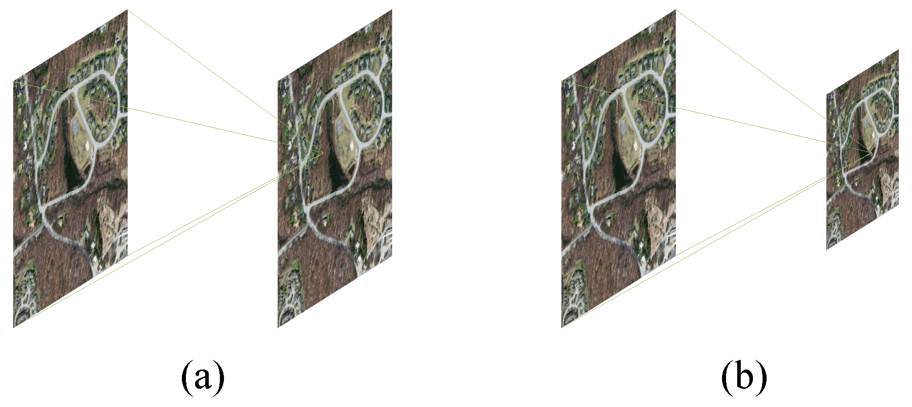
Figure 1. The attention feature maps. (a) The traditional non-local method, where each feature point includes all the information in the current feature map. (b) The core idea of our proposed network. Each feature point of the small-scale feature map is aggregated from the context information of the large-scale feature map.
Remotesensing 15 00003 g001
Figure 2. The overall structure of the proposed CSANet.
Remotesensing 15 00003 g002
Figure 3. The structure of the CFP module. c is the number of channels of the input features.
Remotesensing 15 00003 g003
Figure 4. (a) The structure of the CSA module. F h represents high-resolution features and F l represents low-resolution features. (b) Schematic diagram of matrix multiplication between Q 1 and K 1 in (a). (c) Schematic diagram of matrix multiplication of Q 2 with K 2 in (a).
Remotesensing 15 00003 g004
Figure 5. Visualization of segmentation results generated by different methods on the Massachusetts Roads dataset. (a) Original image. (b) Ground truth. (c) CSANet. (d) Deeplabv3. (e) UNet. (f) ENet. (g) CFPNet. (h) SegNet. (i) PSPNet.
Remotesensing 15 00003 g005
Figure 6. Visualization of segmentation results generated by different methods on the DeepGlobe dataset. (a) Original image. (b) Ground truth. (c) CSANet. (d) Deeplabv3. (e) UNet. (f) ENet. (g) CFPNet. (h) SegNet. (i) PSPNet.
Remotesensing 15 00003 g006
Figure 7. Comparison of our method with the visual segmentation results of CFPNet: the first row is the segmentation results of the Massachusetts Roads dataset; the second row is the segmentation result of DeepGlobe. (a) Original image. (b) Ground truth annotations. (c) Predicted results of CSANet. (d) Predicted results of CFPNet.
Remotesensing 15 00003 g007
Figure 8. Visualization of the ablation study, where the top two rows are segmentation results for the Massachusetts Roads dataset and the bottom two rows are the segmentation results for the DeepGlobe dataset. (a) Original image. (b) Ground truth. (c) No. 1. (d) No. 2. (e) No. 3. (f) No. 4.
Remotesensing 15 00003 g008
Figure 9. Network FLOPs and IoU accuracy.
Remotesensing 15 00003 g009
Figure 10. Network parameter volume and IoU accuracy.
Remotesensing 15 00003 g010
Table 1. Qualitative comparison of the proposed method (CSANet) with other methods on the Massachusetts Roads dataset.
MethodRecallPrecisionIoUIoU r AccuracyF1
Unet [42]68.1578.2357.2984.4998.0672.84
Enet [45]66.0880.6857.0584.5797.1072.65
DeepLabv3 [46]66.5775.9354.9783.6997.9270.95
CFPNet [36]67.7375.8955.7385.1097.9471.57
SegNet [43]66.4778.3056.1382.8498.0271.90
PSPNet [44]66.1974.3753.9085.1497.8470.04
CSANet69.1480.0558.9884.9598.1674.20
Table 2. Qualitative comparison of the proposed method (CSANet) with other methods on the DeepGlobe dataset.
MethodRecallPrecisionIoUIoU r AccuracyF1
Unet [42]57.2378.1549.3369.1598.4866.07
Enet [45]54.5079.0947.6469.3597.4364.53
DeepLabv3 [46]76.0878.6563.0683.1498.0977.34
CFPNet [36]76.2580.7864.5483.9098.2078.45
SegNet [43]61.0174.4050.4367.1897.4367.04
PSPNet [44]69.3877.8657.9577.8697.8473.38
CSANet75.0583.3765.2884.1798.2978.99
Table 3. Ablation study of the CSA module on the Massachusetts Roads dataset.
No.CSA-1CSA-2RecallPrecisionIoUF1
1 67.3279.557.3672.9
2 68.6779.9658.5973.89
3 67.8679.8557.9473.37
469.1480.0558.9874.20
Table 4. Ablation study of the CSA module on the DeepGlobe dataset.
No.CSA-1CSA-2RecallPrecisionIoUF1
1 73.9783.3864.4678.39
2 74.5483.4964.9678.76
3 74.0683.2864.4878.40
475.0583.3765.2878.99
Table 5. Computation complexity and parameter sizes of different methods.
MethodIoUParamFLOPs
UNet57.2928.2 M238.53 G
ENet57.050.36 M2.25 G
DeepLabv354.9754.7 M82.98 G
CFPNet55.730.54 M3.89 G
SegNet56.1329.48 M562.56 G
PSPNet53.9046.71 M184.44 G
CSANet58.980.62 M7.55 G
Disclaimer/Publisher’s Note: The statements, opinions and data contained in all publications are solely those of the individual author(s) and contributor(s) and not of MDPI and/or the editor(s). MDPI and/or the editor(s) disclaim responsibility for any injury to people or property resulting from any ideas, methods, instructions or products referred to in the content.