Abstract
Terracing is widely used as an effective soil and water conservation practice in sloped terrains. Physically based hydrological models are useful tools for understanding the hydrological response of terraced catchments. These models typically require a DEM as input data, whose resolution is likely to influence the model accuracy. The main objective of the present work was to investigate how DEM resolution affects the accuracy of terrain representations and consequently the performance of SWAT hydrological model in simulating streamflow for a terraced eucalypt-dominated catchment (Portugal). Catchment´s hydrological responses were analyzed based on two contrasting topographic scenarios: terraces and no terrace, to evaluate the influence of terraces. To this end, different SWAT models were set up using multi-resolution DEMs (10 m, 1 m, 0.5 m, 0.25 m and 0.10 m) based on photogrammetric techniques and LiDAR data. LiDAR-derived DEMs (terraces scenario) improved topographic surface and watershed representation, consequently increasing the model performance, stage hydrographs and flow-duration curves accuracy. When comparing the contrasting topographic scenarios, SWAT simulations without terraces (10 m and 1 m DEMs) produced a more dynamic and rapid hydrological response. In this scenario, the streamflow was 28% to 36% higher than SWAT simulations accounting for the terraces, which corroborates the effectiveness of terraces as a water conservation practice.
1. Introduction
Terrace, a millennial practice, are manmade structures edified along contours lines on high sloped terrains, typically edified along contour lines for promoting water and soil conservation. Terracing has been largely referred as a sustainable management practice [1,2] being considered an effective nature-based solution to reduce erosion, landslide, and flood risks [3]. The ridges and embankments created by terraces, promote water infiltration [4,5] playing an important role not only in the interception of runoff but also on the stabilization of hillslopes, which further promote the evolution of soil layers, especially on sloped hills with shallow soils or with bare soil backgrounds [6,7]. This practice has also been found to provide other important ecosystem services such as carbon sequestration [8,9,10]. In a recent review paper [11], aside from highlighting the ecological benefits of terraces (e.g., reduction on runoff and promotion of water conservation, erosion control and soil conservation, increase of crop yields, and protection of biodiversity), we have also pointed out their potential disadvantages (e.g., disruption of water circulation, mass movement in poorly designed terraces, and soil erosion after terrace abandonment).
Although there is no standard classification or terminology for terraces [12], suggested their assemblage according to the overall slope ranges. Terraces on steep sloped areas and exceeding 7° (e.g., level bench terraces, upland bench terraces, hillside ditches, orchard terraces). On gentle sloped areas with less than 7° other type of terraces like broad base-graded terraces and broad base-level terraces are commonly found. On steep areas, terraces are used by forest managers when establishing new plantations because aside from the previously mentioned advantages, they allow for terrain levelling and facilitate accomplishment of future management operations (e.g., harvest, logging, clear cuts) [13].
Hydrological models are valuable tools to understand the hydrological functioning of terraced catchments, which is of great relevance for forestry sector.
Physically based hydrological models typically require, as an input, a Digital Elevation Model (DEM) to compute the terrain settings of the study-area. DEM resolution impacts the computation of surface morphometry, influencing the resulting extracted features (e.g., watershed delineation, stream network, slope, aspect and, topographic wetness index). Several studies debate the influence of DEM resolutions on the extracted morphometric features stressing the gains on detail and accuracy [14,15,16,17]. Very high-resolution DEMs have been reported to enhance morphometric, topographic and hydrological features as well as geomorphometric indices (e.g., surface roughness, index of connectivity) [18,19,20]. Buakhao et al. [21] focused on the impacts of DEM resolutions on the definition of watershed physical characteristics with regard to the total streamline length, main channel slope, watershed area and slope, and area slope were significantly more accurate with increasing DEM detail (ranging from 5 to 90 m).
Wu et al. [22] assessed the links between automatic watershed extraction, watershed parameters and area threshold values upon applying a model to 10 catchments with three DEM resolutions, ranging from 250 m, 500 m to 1000 m, and concluded that a DEM increased resolution results in more refined flow direction and accumulation calculations translating in a more realistic stream network representation. Tan et al. [23] achieved overall enhanced streamflow simulations when applying 20 m and 60 m resolution DEMs and enhanced DEM sensitivity analysis.
Goulden et al. [24,25] debated the influence of DEM resolutions on the topographic representation and on the morphometric features and, assessed the relations between DEM resolutions and SWAT outputs. Zhang et al. [26] presented a comprehensive analysis on the influence of 17 DEM resolutions (ranging from 30 to 1000 m) on SWAT simulated hydrological responses. Lin et al. [27] focus on the use of 11 resolution DEMs (ranging from 5 m to 140 m) on the SWAT model predictions for water availability (quantity and quality). In a recent study, Tran et al. [28] presented a comprehensive framework aiming the evaluating of impacts of six global DEMs on SWAT simulated stream flows. Very high-resolution DEMs are able to provide the precise terrace geometry with very accurate georeferenced setting and, therefore, improve hydrological models estimates of surface runoff and percolation, water retention capacity as well as nutrients and sediment exports.
The advent of Airborne Laser Scanning (ALS) sensors coupled in different platforms, such as unmanned aerial vehicles (UAV) and aircrafts, enhanced the panorama of generating DEM’s using point cloud data with high-resolution and a good vertical accuracy when compared with spaceborne DEMs [29]. However, as stressed [30], slope and aboveground vegetation influence the DEM accuracy. Conversely, the accuracy depends on the sensor type, flight height, point density, number of echoes, and scan angle [31,32,33]. LiDAR based data, particularly DEMs has been widely applied in different fields such as in forest characterization [34,35], forest inventories [36], stream network modelling [37], flood monitoring [38], morphometric analysis [39], drainage network analysis [40], and exploration of snow distribution in steep forested slopes [41].
Hydrological models such as the Soil and Water Assessment Tool (SWAT) model have been widely and successfully applied to different biogeographic regions and bioclimatic contexts to simulate the effectiveness of terraces as a water and soil conservation strategy [7,42,43,44]. In the work of [42] a comprehensive description of the parameters used within SWAT to represent terraces was addressed the linked effects on catchment processes were detailed. Shao et al. [7] focused on specific procedures to reproduce physical characteristics of terraces, as a way to improve SWAT simulations of runoff and sediment transport from terraced landscapes. Khelifa et al. [43] debates the influence of proper SWAT parameterization of bench terraces to support large scale modelling of runoff and sediment yields in Tunisia. Another study by Boufala et al. [44] used SWAT to assess the effectiveness of management practices including terraces, on the reduction of water yields and sediment yields in Morocco watershed.
SWAT assumes regular terrace geometry (slope steepness) and divides the hillslope based on the horizontal terrace distance, assuming equal cut and fills of soil volumes for all terraces. As a result, different types of terraces produce similar responses, which can lead to erroneous hydrological simulations and inaccurate assumptions and predictions [6,7]. The use of very high-resolution and very detailed DEMs ensures a more accurate representation of the topographic surfaces and, as a result, a more realistic representation of the terraces which, ultimately will improve the simulation of water dynamics on a terraced catchment.
Despite the influence of DEMs resolution on hydrological modelling, there is only a small number of works addressing this issue for forested terraced catchments. In the present work, the accuracy of multi-resolution DEMs in morphological terrain representations and the associated effects on SWAT model performance was investigated for a eucalypt-dominated terraced catchment in Central Portugal. To this end, various SWAT models were set up using DEM of cell sizes ranging from 10 m, 1 m, 0.5 m, 0.25 m and 0.10 m to evaluate the effects on streamflow estimates and on stage hydrographs.
The present study stresses the added value of using hydrological model simulations (feed by high-resolution remote sensed DEMs) to promote a more sustainable forest management practices in sloped areas.
2. Materials and Methods
2.1. Experimental Catchment
The Braçal experimental catchment is located in Silva Escura (Sever do Vouga municipality, Central mainland Portugal). The catchment covers an area of about 44 ha, draining into the Mau River, a tributary of the Vouga River. Elevations within the catchment range from 180 to 400 m a. s. l.
The area is characterized by a Mediterranean-type climate with an oceanic (Atlantic) influence, classified as a humid mesothermal (tempered) climate (CsB), according to the Köppen [45] classification. The mean annual temperature and rainfall in the area for the period of 2018 to 2022 was, respectively, 15 °C and 1300 mm. The maximum air temperature is typically registered in June–August and the minimum between December and February. The wet period (75% of the total annual rainfall) typically occurs from October to March.
The predominant geological background are metasedimentary rocks from the “Schist-Greywacke Complex” with Pb-(Zn-Ag) hydrothermal vein deposits that have been explored (lead mining) since Roman occupation [46]. The catchment is mainly covered by chloritic, striped, and grey Mesozoic schist intersected by quartz veins, often reaching a breadth of several meters [47].
Soils in the study area are predominantly Humic Leptosols (area without terraces) and Skeletic Escalic Regosols (area with terraces) [48,49,50] These soils are derived from schists with little profile differentiation and being typically shallow soils with silt loam texture. Three soil profile campaigns were carried out within the catchment to produce the digital soil map used as input to the model, and to collect soil data for model parameterization.
Regarding land use, the catchment is largely occupied by evergreen broadleaf species (Eucalyptus globulus Labill; 80%), unpaved roads and firebreaks (7%), mixed forest (6%, largely defined by Acacia dealbata Link and oak), oak trees (5%) and scrubland (2%) (Figure 1).
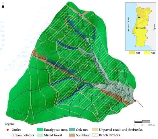
Figure 1.
Location of the Braçal experimental catchment. Representation of the main land uses, stream network, topographic surface and area cover by terraces (0.25 m DEM).
The catchment registers an average slope ranging from 15% to 27%, as the catchment is partially occupied by bench terraces (identified in Figure 1 with a light grey line). Bench terraces are edified along the steeper parts of the catchment and represent about 59% of the total area, being mostly occupied by eucalypt plantation (72%). On the Braçal experimental catchment upland bench terraces, more precisely reverse sloped terraces [12] were edified (Figure 2). These terraces average 2 m in length and 2 m in height.
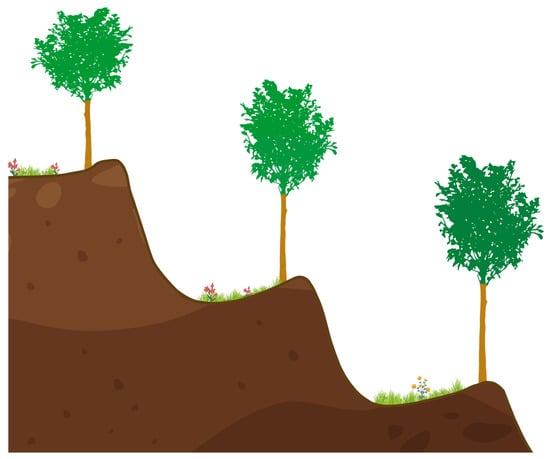
Figure 2.
Schematic representation of the reversed slope terraces edified on the Braçal experimental catchment.
2.2. UAV Data Collection and Processing
The UAV-LiDAR data was acquired in November 2021 through 3 flights. The DJI Matrice 300 (Da Jiang Innovations, Inc., Shenzhen, China) quadcopter unmanned aerial vehicle (UAV) was used in terrain following mode (Figure 3). Using the YellowScan Mapper (YellowScan, Montferrier-sur-Lez, France) coupled which is equipped with a Livox Horizon laser scanner from Livox and a GNSS-Inertial Applanix APX-15 was operated with a flight altitude of 70 m AGL, flight speed 7 m/s, with a swath width of 120 m, and overlap of 50%, with an average point cloud density of approximately 320 pts/sqm. This sensor records 240 k shots per second and up two echoes of pulse. Regarding to the wavelength is 905 nm with a reproducibility of 2 cm and 3 cm of accuracy. The DJI Terra software (Version 3.0, Da Jiang Innovations, Inc., Shenzhen, China) was used to set up the drone and cameras.
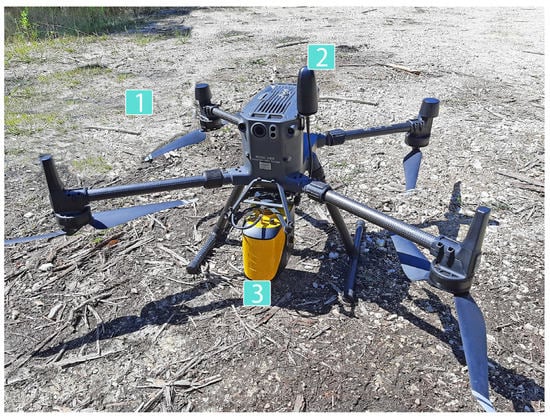
Figure 3.
Unmanned aerial vehicle (UAV) used to collect LiDAR point clouds: (1) Matrice 300 RTK; (2) YellowScan RTK Antenna; (3) YellowScan Mapper.
The UAV-LiDAR postprocessing phase was performed with YellowScan CloudStation software. Automatic strip generation and production of LASer (LAS) files were the first procedures after the LiDAR data collection. Depending on surface sector, the usage of UAV terrain following mode allows a good distribution of points and scan angle ranging from 20% to 40%.
The FUSION/LDV software of the USDA Forest Service [51] as used to extract bare-earth DEM surfaces in dense point clouds. The workflow was as follows:
(i) Filter data (Filterdata FUSION/LDV tool) to remove outliers and overlayed return data, that works by computing the mean elevation and standard deviation of elevations for each cell in the comparison grid;
(ii) Ground filter to identify the returns which are likely to form the surface (bare-earth points) using different cell size (windows size) measures (0.1 m, 0.25 m, 0.5 m, and 1 m) and a constrained tolerance value for the final filtering of ground points. The ground filtering algorithm used is available in the GroundFilter tool implemented in FUSION/LDV, which is Weighted Linear Least Squares (WLS), and it combines filtering and interpolation procedures;
(iii) Conversion of the DEM file format obtained from the ground filter step to an ASCII file. This step was essential to observe the returns not completely removed in QGIS software;
(iv) Visualization and identification of returns not completely removed in QGIS, namely the vegetation in water lines such as Acacia dealbata and scrubs;
(v) Finally, the no bare earth points were manually removed using the CloudCompare [52] software, and the workflow started again in step (ii), until all the ground points were removed. This iterative process was done to produce 0.1 m, 0.25 m, 0.5 m, and 1 m bare earth DEMs.
2.3. DEM Build-Up
The DEM resolutions considered in this study aimed two represent contrasting topographic scenarios: (1) the presence of terraces (in 59% of the area, representing the actual topography) and (2) the absence of terraces (no terrace).
To accurately capture the terraces, four very high-resolution DEMs (1 m, 0.5 m, 0.25 m, and 0.10 m), based on a Light Detection and Ranging (LiDAR) survey (Ls) were built up (Figure 4).
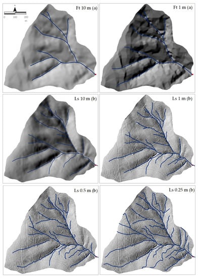
Figure 4.
DEMs for the Braçal catchment: (a) 10 m and 1 m Ft DEMs; (b) 10 m, 1 m, 0.5 m, 0.25 m Ls DEMs.
The absence of terraces was reflected in two DEM resolutions: 10 m and 1 m. DEMs interpolated with 10 m equidistant contour lines obtained via photogrammetric techniques (Ft) (Portuguese Geographical Institute, National Cartography Series, map no. 175-1:10,000 scale) based on two premises: (a) the lack of proper cartographic resolution to represent terraces and (b) the 10 m contour lines were produced around 1995/1996 when no terraces were yet defined within the catchment. In addition, a 10 m Ls DEM was defined to for no terrace scenario to get proper comparation with the 10 m Ft DEM. This 10 m Ls DEM is based on the same input data that provided the Ls DEMs. In this sense, the actual topographic setting is the same differencing in the pixel size for the produced DEMs. The 10 m Ls DEM focuses on the use of a topographic surface that was generated without considering the actual physical existence of bench terraces analyses due to a coarser cell size.
For the 10 m and 1 m Ls DEMs the pixels were downscaled to compare resolutions and provide valuable insights on topographic surfaces and morphometric features. The input data for the Ls and Ft DEMs was computed by a triangulated irregular network surface through the Delaunay triangulation and converted to raster. The 10 m and 1 m (Ft and Ls) DEMs denote similar horizontal resolutions but are based on different acquisition methods (LiDAR and photogrammetry) and production scales, providing differential morphometric and hydrological responses.
The input data for the Ft DEM dates back to the middle 1990s, whereas Ls DEMs were built based on data collected in late 2021.
For each DEM, the stream networks were calculated using the D8 hydrological algorithm [53] provided by the Terrain Analysis Using Digital Elevation Models (TauDEM), and their accuracy was assessed based on: drainage density (Dd: average total stream length/catchment area, with a higher value representing a more agglutination of the channels), sinuosity (S: length of meandering/straight-line distance, with zero indicating a curvy line), vertex index (Vi: number of vertices/total stream length, with zero indicating poor complexity, with no curvy lines), and the bifurcation ratio (number of stream network segments of a given Strahler order divided by the number of divisions on a higher order) [54,55,56].
The stream network obtained by LiDAR was further validated with orthophoto imagery from a UAV survey held in the catchment area in November 2021. The rectified and validated stream network generated with the 0.25 m DEM was used to calculate the matching degree between the reference (actual) stream network and the other DEM resolution extracted networks [57,58].
2.4. Hydrological Modeling
2.4.1. SWAT Setup and Parametrization
SWAT is a time-continuous, physically based and semi-distributed model that allows the simulation of landscape processes and catchment responses, from a sub-daily to the yearly basis [59,60]. SWAT uses small detailed spatial units, named Hydrologic Response Units (HRUs), by overlaying land use/cover types, soil types and slopes classes. The model simulates processes from the HRU level up to the watershed scale [61,62]. Several inputs and parameters are required for model build-up—namely, a DEM; a soil map; a land use/land cover map; and meteorological data (specifically, rainfall, minimum and maximum air temperature, relative humidity, wind speed and direction, and solar radiation).
For catchment delineation, a pre-defined watershed (0.25 m Ls DEM) limit was used following the approaches of Luo et al. [63] and Rocha et al. [64]. The automatic delineation process can lead to misrepresentations of the real watershed limit with some sector being defined outside the actual limit or cutting-off parts of the watershed resulting, on an increase or decrease of the actual area, as stressed by Śliwiński et al. [65].
The DEM is one of the first inputs added in the model to support simulations. Six individual SWAT models were set up using the 10 m and 1 m Ft DEMs and 10 m, 1 m, 0.5 m and 0.25 m Ls DEMs.
SWAT databases included site-specific parameters, namely related to soils and eucalypt ecophysiology, which were obtained, respectively, from field work surveys and by destructive and non-destructive forest inventories. The eucalypt operation schedule (e.g., plant/begin growing season, harvest index target) was defined by date to preserve observed meteorological conditions. The silviculture operations (SWAT management operations) for the eucalypt stands within the catchment were established considering The Navigator Company operational practices. General plant parameters and management operations were defined based on the SWAT database and adapted from previous studies [16,17,64,66,67,68].
Sub-hourly meteorological data (e.g., rainfall, air temperature, air humidity, solar radiation, wind speed and direction) were provided by one automatic meteorological station installed within the catchment area. Sub-hourly streamflow data was provided by an automatic hydrometric station installed on an H-flume at the catchment outlet.
SWAT2012 was run on a daily basis from 2012 to 2022 with seven years of warm-up to minimize initial effect of catchment dynamics and to ensure model stabilization.
For the no terrace scenario the input DEM resolution lacked the authentic morphological and topographical effect of terraces, SWAT was parametrized to simulate terraces by fine-tuning of erosion and runoff parameters (e.g., USLE practice factor, average slope length, initial curve number, initial SCS runoff curve number for moisture condition II; [62,69].
2.4.2. Model Calibration and Performance Assessment
Model calibration is influenced by the uncertainties of the input data and model results tend to be different for each of the input DEMs. For this reason, the same SWAT parameters were assumed for each model when running the model with the different DEMs, to minimize model uncertainty.
To fully understand the constrains provided by the DEM resolutions, a preliminary assessment was performed considered by comparing the overall model results based on a non-calibrated approach. This hypothetical scenario lacked a fine-tuning terrace-associated parameters (since it used default values) providing insights on the mismatch of the observed and simulated data and on the influence of terraces, in line with what was proposed by Khelifa et al. [43].
The model was calibrated using streamflow data collected at the catchment outlet from March 2019 to May 2022. Using the 0.25 m DEM as reference, the SWAT was first manually calibrated to narrow the parameter ranges, and latter was automatically calibrated using the Calibration and Uncertainty Analysis Program (SWAT-CUP; [70]). This calibration procedure defined the SWAT parameters that were used for the different models built from different DEMs. SWAT-CUP is an iterative calibration procedure that allows the use of optimization algorithms and objective functions to simultaneously calibrate multiple parameters. For the calibration routines, it was used the Sequential Uncertainty Fitting algorithm (SUFI2—[60,71] to perform not only the calibration, but also a sensitivity analysis and an uncertainty analysis. SUFI2 was run with 3 iterations each comprehending 440 simulations.
Four goodness-of-fit indicators were used to assess model performance: (i) the average percent model error (PBIAS—percentage of bias), with zero (optimal value) indicating a perfect fit and, positive and negatives values indicating, respectively, model underestimation and overestimation; (ii) the Nash-Sutcliffe model efficiency index (NSE) ranging from one (optimal value) to −∞ (unacceptable model calibration); (iii) the Coefficient of Determination (R2) multiplied by the coefficient of the regression line (bR2), ranging from one (optimal value) to zero; and (iv) the Kling-Gupta efficiency index (KGE) ranging from one (optimal value) to −0.41 [64,65,66,67].
The ranges of the goodness-of-fit indicators used for evaluating model performance were adapted from Moriasi et al. ([72,73,74,75]: Table 1).

Table 1.
Goodness-of-fit indicators for evaluating the performance of hydrological models for streamflow (adapted from Moriasi et al. [74,75]).
3. Results and Discussion
3.1. Effects of DEM Resolution on Surface and Morphometric Features
The coarser resolution 10 m Ls and Ft DEMs generated topographic surfaces and morphometric features that were not able to represent the terrace’s location and geometry and did not fully account for the significance on the runoff misestimating catchment overall hydrological responses.
In general, an increase in DEM resolution gradually improved the accuracy of the extracted morphometric features (Table 2).
Table 2.
Morphometric features for the LIDAR (Ls) and photogrammetric (Ft) DEMs.
The altimetry amplitude of the catchment was proved to be incitingly more accurate with increasing DEM resolution. The coarser resolutions, denoted an altimetry detail loss on the maximum and minimum elevation values as a result of both underestimation and overestimation routines, as reported by Zhang et al. [25] and Reddy et al. [76].
The Ls 1 m and 10 m DEMs achieved slightly enhanced accuracy namely on the drainage density, sinuosity and matching degree. For the same scale range (1 m and 10 m) a parallel visual analysis highlights the details gains achieved on topographic surface representation by Ls DEMs when compared with the Ft DEMs.
The drainage density and sinuosity were also more accurate for the Ls DEMs with the highest resolution, especially when compared with the Ft DEMs.
The Ft DEMs registered a total watershed area of 36.12 ha and 38.77 ha, respectively, for the 10 m and 1 m DEMs.
The Ls DEMs registered a more reduced gap for the on the total catchment areas, ranging from the 42.18 ha, 42.36 ha, 42.54 ha, and 42.89 ha, respectively, for the 10 m, 1 m, 0.5 m, and 0.25 m DEMs (Figure 4).
The 0.10 m Ls DEM denoted some incongruences on the actual representation of the topographic surface and morphometric features. These constrains may be linked with dense vegetation that inhibits laser ground return signal and with the two individual returns (low density number of returns) per pulse from the LiDAR survey. Dense canopy and ground vegetation can reduce the penetration of LiDAR pulses to the ground especially on complex topography and dense vegetation cover regions [77,78,79]. Constrains imposed by vegetation patterns in the actual topographic surface representation were also reported by Goulden et al. [24,25], while White et al. [80] found similar constrains of terrain representation using a low-density LiDAR survey. Thus, this very high-resolution 0.10 m DEM did not result in additional gains on the surface representation, on the catchment morphometric features and on streamflow representation. This 0.10 m DEM seems not to be suitable for proper stream flow representation due to erroneous flow patch and direction calculations. The 0.10 m DEM extracted stream network represented, in specific sectors, channel lines according to the topographic surface with no running free flow on all channels. The decreased accuracy at 0.10 m DEM may be caused by geomorphological micro-scale variations (“noise”) provided by real-world topographic variation or by artifacts of DEM generation, as reported by Baltensweiler et al. [81]. The 0.10 m DEM was not considered for these analyses due to the above-mentioned incongruences. As a result, the 0.25 m DEM was defined as the reference for this work as this DEM proved to be the most reliable and accurate for representing the topographic surface.
The 0.25 m DEM extracted features (e.g., stream network, slope) were also explored with the D∞ method [82] but the involved computation cost and the overall result denoted no additional gains, in line with suggested by Yang et al. [83].
The stream network tended be more detailed for the very high-resolution Ls DEMs (Figure 5), as several streamlines are narrower than the 0.5 m pixel size input DEM data and may not be totally accounted by coarser topographic settings.
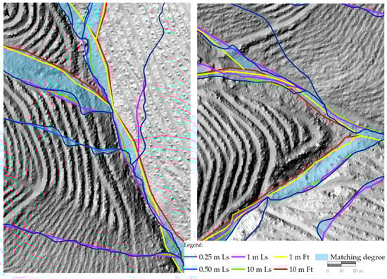
Figure 5.
Matching degree of the extracted stream networks for the different DEMs considering the 0.25 m Ls DEM as a reference.
3.2. SWAT Perfomance
Previous modelling approaches stressed the importance of using non-calibrated models rather than fine-tuned models to better account for the effect of medium-to high-resolution DEMs [77,84]. Although the 10 m Ls and the Ft DEMs were unable to represent terraces, the model performance was still rated as satisfactory. The simulations within the terrace scenario denoted an increased model performance associated to the DEM improved accuracy. These simulations registered an improved rank for the goodness-of-fit indicators (PBIAS, NSE, bR2, and KGE) with the 0.25 DEM and achieved higher overall model performance, due to a more accurate representation of the terraces and the overall catchment characteristics. These results are corroborated by the increased improvements on the representation of the topographic surface and morphometric features by means of gradually applying more detailed very high-resolution DEMs.
The simulations with the 10 m Ls DEM, however, were slightly more accurate than those using the Ft DEMs. These findings seem to be related to the detail imposed by the LiDAR survey and to the enhanced capability to represent the actual topographic surface and the extracted morphometric features. When comparing the 10 m Ls and Ft DEMs, it became obvious that despite having the same spatial resolution (cell size) the very high-resolution of the LiDAR produced enhanced SWAT stream flow simulations and impacted the overall model performance, as supported by the goodness-of-fit indicators presented in Table 1.
The no terrace scenario denoted satisfactory model performance, although simulations with the Ls DEM showed slight better performance when compared with the Ft DEMs (Table 3).
Table 3.
Goodness-of-fit indicators for model performance when using LIDAR (Ls) and photogrammetric (Ft) DEMs as input for SWAT.
As model parameters were the same for both the Ft and Ls DEM simulations, these results were to be expected, as stressed by Strehmel et al. [85] and Roostaee et al. [86].
If some specific SWAT parameters, such as SURLAG (surface runoff lag coefficient), GW_DELAY (time that the water released by the soil bottom layer needs to reach shallow aquifer) and runoff curve number [62,87] were fine-tuned, model performance would be better. A lower SURLAG value means more water storage over time resulting in smoother streamflow hydrographs. A reduced GW_delay (e.g., 1, 2) value mimics conditions of more permeability and results in different water availability affecting peaks runoff rate and base-flow rates.
3.3. Effects of DEM Resolution on the Catchment Hydrological Responses
For the no terraces scenario (Ft DEMs and 10 m Ls DEM), the overall streamflow was 28 to 36% higher than in the terrace scenario (Figure 6 and Figure 7; Ls DEMs). In the absence of terraces, the model response to rainfall events was more dynamic, likely because of the reduced water concentration time (Figure 6 and Figure 7). These findings reinforce the importance of terraces as a water conservation practice.
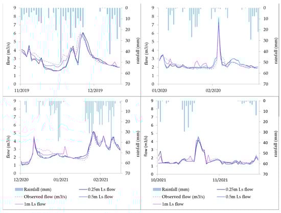
Figure 6.
Observed and simulated streamflow for the terrace’s scenarios (0.25 m, 0.50 m, and 1 m Ls DEMs), from November 2019 to November 2021.
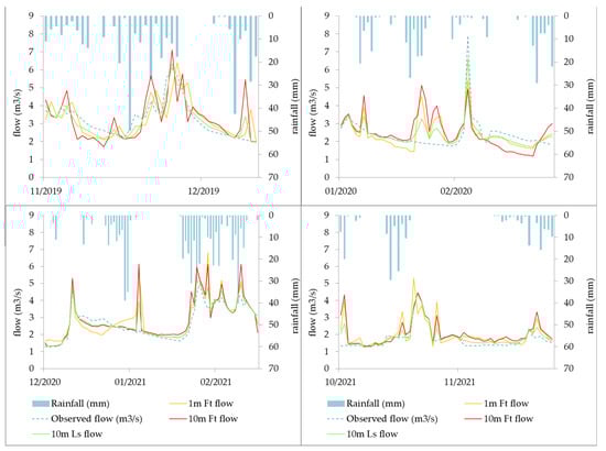
Figure 7.
Observed and simulated streamflow for the no terraces scenarios (1 m and 10 m Ft DEMs, and 10 m Ls DEM), from November 2019 to November 2021.
For the terrace scenario, the increasing DEM resolution denoted gains on streamflow simulation due to the increased realism of topographic and morphometric features, which possibly enhanced the representation of the water connectivity patterns within the catchment. These findings, however, contrast with previous research from Goulden et al. [24] using a 1 m DEM and Kumar et al. [88] with 16 DEMs (from 40 m to 1000 m), where the authors referred that DEM have a negligible effect on streamflow reduction, although these studies are not addressed in terraced catchments. Lin et al. [89] and Zhang et al. [26] have also reported little influence on SWAT-simulated streamflow by improving DEM resolution, but these authors used coarser cell sizes than in the present study, respectively, from 5 to 140 m and from 30 to 1000 m.
Overall, the stage hydrographs for the all period of the different DEMs tended to mimic some responses to rainfall events since the hydrographs for the different DEMs overlap (Figure 6 and Figure 7). However, when analyzing only the hydrographs of the bigger rainfall events, differences between DEMs were noticeable. For the Ls DEMs, the increasing resolution translated into a more realistic representation of streamflow peaks and a delay on the time to peak, when compared with the observed records. For the Ft DEMs, the decreased resolution translates into more erratic overall streamflow representation, with higher stream flow peaks and a more rapid responses to rainfall events with several irregular and anticipated peaks when compared with the observed records or the 0.25 m reference DEM.
Assuming the 0.25 Ls DEM as the reference simulation, normalized flow-duration curves were constructed using the results of daily streamflow simulations under the different DEMs (Figure 8). The results showed a good agreement between the flow-duration curves of the different DEMs, which is in line with the good model performance achieved by the different SWAT models (Table 2).
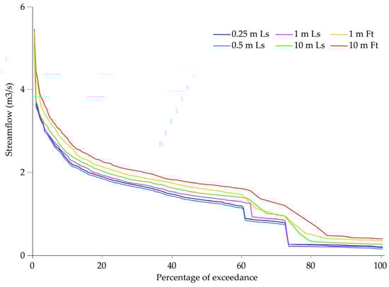
Figure 8.
Normalized flow-duration curves for the terraces (Ls DEMs) and no terraces (10 m and 1 m Ft DEM and 10 m Ls DEM) scenarios.
When analyzing the flow-duration curves for the terraces (Ls DEMs) and no terraces (10 m and 1 m Ft DEM and 10 m Ls DEM) scenarios, some differences became evident. The presence of terraces seems to reduce streamflow as also pointed out by other authors [90,91,92].
The curves for the 0.25 m and 0.50 m DEMs were very similar as would be expected since the topographic surfaces and morphometric features were also similar (Figure 4). Differences between flow-duration curves tend to be more evident on the 60% to 85% exceedance interval, where little variability between curves was observed for the exceedance intervals of 0–10% and 85–100% exceedance level for both scenarios (terrace and no terrace).
4. Limitations to the Work
The postprocessing LiDAR data on this sloped forest catchment demanded a high computation cost and as a result was necessary to execute a partition of the point clouds in several smaller parts in order to produce the necessary DEMs. Conversely, low number of echoes of pulse (maximum of two echoes) scan angle, slope, and very dense canopy, due to stands ages and aboveground vegetation, in some sectors of the catchment may have played an important role on the final accuracy of the produced DEMs and on the extracted features (e.g., stream network, slopes).
The lack of multi-depth soil moisture sensors within the catchment was also a limitation to model parameterization and performance. Actual soil moisture data gather within terraced areas could enhanced model parameterization and improve simulation results. In turn, overall model performance can gain from additional use of data as calibration was not solely based on outlet streamflow data.
The fact that model parameters were similar for the different DEMs influenced model performance. If the different SWAT models were individually fine-tuned, the accuracy of model simulations would have likely improved.
The limited streamflow dataset is also a major drawback of the present work. A larger data set, including several wet and dry years, would have increased the robustness of the calibration. Ideally, the model should also have been validated to improve the confidence in its ability to reproduce the catchment hydrological processes. The model uncertainties associated to flow measurements are also worth to be highlighted. Rainfall events tend to stop from late May to mid-October reducing the overall quantity of available free flow in the catchment. Within this period, some sporadic rainfall events might not have been able to generate water levels to be recorded by H-flume sensors, which influenced the total amount of annual streamflow measured.
5. Conclusions
In this study an exploratory ecohydrological modelling approach coupled with remotely sensed high to very high-resolutions DEMs to simulate two contrasting topographic surfaces defined by the presence of bench terraces and the absence of terraces on a eucalyptus dominated catchment. The multi-resolution DEMs (provided by Lidar and photogrammetric techniques) used as input for the SWAT model provided valuable insights on the potential role of bench terraces as a sustainable water conservation practice on a forest-dominated catchment.
The 0.10 m LiDAR-derived DEM denoted some incongruences concerning the representation of the topographic surface and morphometric features and produced only minor improvements in model performance when compared to the 0.25 m DEM. In this sense, the 0.25 m was defined as a reference for the modelling approach.
The presence of bench terraces in 59% of the catchment area points to a reduction of 28 to 36% in the streamflow when compared with the no terrace scenario. The SWAT simulated hydrological responses embodied by stage hydrographs and flow-duration curves demonstrated more dynamic and rapid responses to rainfall events, potentially denoting a more reduced water storage capacity because of the absence of terraces.
Future modelling approaches coupled with soil moisture data (obtained from terraced and no terraced catchment sectors) and with a LiDAR survey with five echoes will enhance the SWAT performance.
The SWAT ecohydrological model provided valuable insights on the hydrological responses of a forest-dominated and terraced catchment and as proven to be an added-value for research on forest hydrology, to simulate different scenarios and to be used as a suitable decision-support tool for forest managers and owners.
Author Contributions
Conceptualization, J.R., A.Q. and D.S.; Data curation, J.R. and A.D.; Formal analysis, J.R. and A.D.; Investigation, J.R., A.D., A.Q. and D.S.; Methodology, J.R., A.Q. and D.S.; Software, J.R. and A.D.; Validation, J.R.; Visualization, J.R.; Resources, A.Q. and S.F.; Project administration A.Q. and S.F.; Supervision, A.Q., D.S. and S.F.; Writing—original draft, J.R.; and Writing—review and editing, J.R., A.D., A.Q., D.S. and S.F. All authors have read and agreed to the published version of the manuscript.
Funding
The author (Dalila Serpo) would like to acknowledge the financial support of CESAM (UIDP/50017/2020+UIDB/50017/2020+LA/P/0094/2020) by FCT/MCTES, through national funds. Dalila Serpa was funded by national funds (OE) through FCT, I.P., in the scope of the framework contract foreseen in the numbers 4, 5, and 6 of article 23 of the Decree-Law 57/2016, of 29 August, changed by Law 57/2017, of 19 July.
Data Availability Statement
Not applicable.
Acknowledgments
The authors would like to express appreciation for the efforts from Bruna Scarparo, Célia Fernandes, Fernando Arede and Filipe Louro on data collection and hydrological survey and Luis Munoz on LiDAR data collection and processing.
Conflicts of Interest
The authors declare no conflict of interest.
References
- Chen, D.; Wei, W.; Chen, L. Effects of terracing practices on water erosion control in China: A meta-analysis. Earth-Sci. Rev. 2017, 173, 109–121. [Google Scholar] [CrossRef]
- Khelifa, W.B.; Strohmeier, S.; Benabdallah, S.; Habaieb, H. Evaluation of bench terracing model parameters transferability for runoff and sediment yield on catchment modelling. J. Afr. Earth Sci. 2021, 178, 104177. [Google Scholar] [CrossRef]
- World Bank. A Catalogue of Nature-Based Solutions for Urban Resilience; World Bank: Washington, DC, USA, 2021. [Google Scholar]
- Wei, W.; Chen, D.; Wang, L.; Daryanto, S.; Chen, L.; Yu, Y.; Feng, T. Global synthesis of the classifications, distributions, benefits and issues of terracing. Earth-Sci. Rev. 2016, 159, 388–403. [Google Scholar] [CrossRef]
- Moreno-de-las-Heras, M.; Lindenberger, F.; Latron, J.; Lana-Renault, N.; Llorens, P.; Arnáez, J.; Romero-Díaz, A.; Gallart, F. Hydro-geomorphological consequences of the abandonment of agricultural terraces in the Mediterranean region: Key controlling factors and landscape stability patterns. Geomorphology 2019, 333, 73–91. [Google Scholar] [CrossRef]
- Yang, Q.; Zhao, Z.; Chow, T.L.; Rees, H.W.; Bourque, C.P.A.; Meng, F.R. Using GIS and a digital elevation model to assess the effectiveness of variable grade flow diversion terraces in reducing soil erosion in northwestern New Brunswick, Canada. Hydrol. Process. Int. J. 2009, 23, 3271–3280. [Google Scholar] [CrossRef]
- Shao, H.; Baffaut, C.; Nelson, N.O.; Janssen, K.A.; Pierzynski, G.M.; Barnes, P.L. Development and application of algorithms for simulating terraces within SWAT. Trans. ASABE 2013, 56, 1715–1730. [Google Scholar]
- Garcia-Franco, N.; Wiesmeier, M.; Goberna, M.; Martínez-Mena, M.; Albaladejo, J. Carbon dynamics after afforestation of semiarid shrublands: Implications of site preparation techniques. For. Ecol. Manag. 2014, 319, 107–115. [Google Scholar] [CrossRef]
- Chen, D.; Wei, W.; Daryanto, S.; Tarolli, P. Does terracing enhance soil organic carbon sequestration? A national-scale data analysis in China. Sci. Total Environ. 2020, 721, 137751. [Google Scholar] [CrossRef] [PubMed]
- Zhao, P.; Fallu, D.J.; Cucchiaro, S.; Tarolli, P.; Waddington, C.; Cockcroft, D.; Snape, L.; Lang, A.; Doetterl, S.; Brown, A.G.; et al. Soil organic carbon stabilization mechanisms and temperature sensitivity in old terraced soils. Biogeosciences 2021, 18, 6301–6312. [Google Scholar] [CrossRef]
- Deng, C.; Zhang, G.; Liu, Y.; Nie, X.; Li, Z.; Liu, J.; Zhu, D. Advantages and disadvantages of terracing: A comprehensive review. Int. Soil Water Conserv. Res. 2021, 9, 344–359. [Google Scholar] [CrossRef]
- Schiechtl, H.M. FAO Watershed Management Field Manual: Vegetative and Soil Treatment Measures (No. 1–5); Food and Agriculture Organization of the United Nations: Rome, Italy, 1985; Volume 13/1.
- Stavi, I.; Fizik, E.; Argaman, E. Contour bench terrace (shich/shikim) forestry systems in the semi-arid Israeli Negev: Effects on soil quality, geodiversity, and herbaceous vegetation. Geomorphology 2015, 231, 376–382. [Google Scholar] [CrossRef]
- Sørensen, R.; Seibert, J. Effects of DEM resolution on the calculation of topographical indices: TWI and its components. J. Hydrol. 2007, 347, 79–89. [Google Scholar] [CrossRef]
- Vaze, J.; Teng, J.; Spencer, G. Impact of DEM accuracy and resolution on topographic indices. Environ. Model. Softw. 2010, 25, 1086–1098. [Google Scholar] [CrossRef]
- Rocha, J.; Duarte, A.; Fabres, S.; Quintela, A.; Serpa, D. Water yield and biomass production on a eucalypt-dominated Mediterranean catchment under climate change scenarios. J. For. Res. 2022. [Google Scholar] [CrossRef]
- Rocha, J.; Duarte, A.; Silva, M.; Fabres, S.; Vasques, J.; Revilla-Romero, B.; Quintela, A. The importance of high resolution digital elevation models for improved hydrological simulations of a mediterranean forested catchment. Remote Sens. 2020, 12, 3287. [Google Scholar] [CrossRef]
- Zhao, H.; Fang, X.; Ding, H.; Strobl, J.; Xiong, L.; Na, J.; Tang, G. Extraction of terraces on the Loess Plateau from high-resolution DEMs and imagery utilizing object-based image analysis. ISPRS Int. J. Geo-Inf. 2017, 6, 157. [Google Scholar] [CrossRef]
- López-Vicente, M.; Álvarez, S. Influence of DEM resolution on modelling hydrological connectivity in a complex agricultural catchment with woody crops. Earth Surf. Process. Landf. 2018, 43, 1403–1415. [Google Scholar] [CrossRef]
- Tarolli, P.; Cavalli, M.; Masin, R. High-resolution morphologic characterization of conservation agriculture. Catena 2019, 172, 846–856. [Google Scholar] [CrossRef]
- Buakhao, W.; Kangrang, A. DEM resolution impact on the estimation of the physical characteristics of watersheds by using SWAT. Adv. Civ. Eng. 2016, 2016, 8180158. [Google Scholar] [CrossRef]
- Wu, M.; Shi, P.; Chen, A.; Shen, C.; Wang, P. Impacts of DEM resolution and area threshold value uncertainty on the drainage network derived using SWAT. Water SA 2017, 43, 450. [Google Scholar] [CrossRef]
- Tan, M.L.; Ramli, H.P.; Tam, T.H. Effect of DEM resolution, source, resampling technique and area threshold on SWAT outputs. Water Resour. Manag. 2018, 32, 4591–4606. [Google Scholar] [CrossRef]
- Goulden, T.; Hopkinson, C. Mapping simulated error due to terrain slope in airborne lidar observations. Int. J. Remote Sens. 2014, 35, 7099–7117. [Google Scholar] [CrossRef]
- Goulden, T.; Hopkinson, C.; Jamieson, R.; Sterling, S. Sensitivity of DEM, slope, aspect and watershed attributes to LiDAR measurement uncertainty. Remote Sens. Environ. 2016, 179, 23–35. [Google Scholar] [CrossRef]
- Zhang, P.; Liu, R.; Bao, Y.; Wang, J.; Yu, W.; Shen, Z. Uncertainty of SWAT model at different DEM resolutions in a large mountainous watershed. Water Res. 2014, 53, 132–144. [Google Scholar] [CrossRef]
- Lin, S.; Jing, C.; Chaplot, V.; Yu, X.; Zhang, Z.; Moore, N.; Wu, J. Effect of DEM resolution on SWAT outputs of runoff, sediment and nutrients. Hydrol. Earth Syst. Sci. Discuss. 2010, 7, 4411–4435. [Google Scholar]
- Tran, T.H.D.; Nguyen, B.Q.; Vo, N.D.; Le, M.H.; Nguyen, Q.D.; Lakshmi, V.; Bolten, J.D. Quantification of global Digital Elevation Model (DEM)–A case study of the newly released NASADEM for a river basin in Central Vietnam. J. Hydrol. Reg. Stud. 2023, 45, 101282. [Google Scholar] [CrossRef]
- Trepekli, K.; Balstrøm, T.; Friborg, T.; Fog, B.; Allotey, A.N.; Kofie, R.Y.; Møller-Jensen, L. UAV-borne, LiDAR-based elevation modelling: A method for improving local-scale urban flood risk assessment. Nat. Hazards 2022, 113, 423–451. [Google Scholar] [CrossRef]
- Stereńczak, K.; Ciesielski, M.; Balazy, R.; Zawiła-Niedźwiecki, T. Comparison of various algorithms for DTM interpolation from LIDAR data in dense mountain forests. Eur. J. Remote Sens. 2016, 49, 599–621. [Google Scholar] [CrossRef]
- Baltsavias, E.P. Airborne laser scanning: Existing systems and firms and other resources. ISPRS J. Photogramm. Remote Sens. 1999, 54, 164–198. [Google Scholar] [CrossRef]
- Hyyppä, H.; Yu, X.; Hyyppä, J.; Kaartinen, H.; Kaasalainen, S.; Honkavaara, E.; Rönnholm, P. Factors affecting the quality of DTM generation in forested areas. Int. Arch. Photogramm. Remote Sens. Spat. Inf. Sci. 2005, 36, 85–90. [Google Scholar]
- Estornell, J.; Ruiz, L.A.; Velázquez-Martí, B.; Hermosilla, T. Analysis of the factors affecting LiDAR DTM accuracy in a steep shrub area. Int. J. Digit. Earth 2011, 4, 521–538. [Google Scholar] [CrossRef]
- Popescu, S.C. Estimating biomass of individual pine trees using airborne lidar. Biomass Bioenergy 2007, 31, 646–655. [Google Scholar] [CrossRef]
- Wulder, M.A.; White, J.C.; Nelson, R.F.; Næsset, E.; Ørka, H.O.; Coops, N.C.; Hilker, T.; Bater, C.W.; Gobakken, T. Lidar sampling for large-area forest characterization: A review. Remote Sens. Environ. 2012, 121, 196–209. [Google Scholar] [CrossRef]
- Tinkham, W.T.; Smith, A.M.; Hoffman, C.; Hudak, A.T.; Falkowski, M.J.; Swanson, M.E.; Gessler, P.E. Investigating the influence of LiDAR ground surface errors on the utility of derived forest inventories. Can. J. For. Res. 2012, 42, 413–422. [Google Scholar] [CrossRef]
- Murphy, P.N.; Ogilvie, J.; Meng, F.R.; Arp, P. Stream network modelling using lidar and photogrammetric digital elevation models: A comparison and field verification. Hydrol. Process. Int. J. 2008, 22, 1747–1754. [Google Scholar] [CrossRef]
- Turner, A.B.; Colby, J.D.; Csontos, R.M.; Batten, M. Flood modeling using a synthesis of multi-platform LiDAR data. Water 2013, 5, 1533–1560. [Google Scholar] [CrossRef]
- Esin, A.İ.; Akgul, M.; Akay, A.O.; Yurtseven, H. Comparison of LiDAR-based morphometric analysis of a drainage basin with results obtained from UAV, TOPO, ASTER and SRTM-based DEMs. Arab. J. Geosci. 2021, 14, 1–15. [Google Scholar] [CrossRef]
- Lyu, F.; Xu, Z.; Ma, X.; Wang, S.; Li, Z.; Wang, S. A vector-based method for drainage network analysis based on LiDAR data. Comput. Geosci. 2021, 156, 104892. [Google Scholar] [CrossRef]
- Koutantou, K.; Mazzotti, G.; Brunner, P.; Webster, C.; Jonas, T. Exploring snow distribution dynamics in steep forested slopes with UAV-borne LiDAR. Cold Reg. Sci. Technol. 2022, 200, 103587. [Google Scholar] [CrossRef]
- Arabi, M.; Frankenberger, J.R.; Engel, B.A.; Arnold, J.G. Representation of agricultural conservation practices with SWAT. Hydrol. Process. Int. J. 2008, 22, 3042–3055. [Google Scholar] [CrossRef]
- Khelifa, W.B.; Hermassi, T.; Strohmeier, S.; Zucca, C.; Ziadat, F.; Boufaroua, M.; Habaieb, H. Parameterization of the effect of bench terraces on runoff and sediment yield by SWAT modeling in a small semi-arid watershed in Northern Tunisia. Land Degrad. Dev. 2017, 28, 1568–1578. [Google Scholar] [CrossRef]
- Boufala, M.H.; El Hmaidi, A.; Essahlaoui, A.; Chadli, K.; El Ouali, A.; Lahjouj, A. Assessment of the best management practices under a semi-arid basin using SWAT model (case of M’dez watershed, Morocco). Model. Earth Syst. Environ. 2022, 8, 713–731. [Google Scholar] [CrossRef]
- Köppen, W. Grundriss der Klimakunde; Walter de Gruyter: Berlin, Germany, 1931; p. 388. [Google Scholar]
- Martins, C.M.B. The Mining Complex of Braçal and Malhada, Portugal: Lead Mining in Roman Times and Linking Historical Social Trends–Amphitheatre Games. Eur. J. Archaeol. 2010, 13, 195–216. [Google Scholar] [CrossRef]
- Ribeiro, C. Relatório sobre as minas de chumbo do Braçal. In Arquivo Técnico do Instituto Geológico e Mineiro (Pasta 226); Technical Archive of the Geological and Mining Institute: Lisboa, Portugal, 1853; p. 24. [Google Scholar]
- SROA. Carta dos Solos de Portugal. I Vol: Classificação e Caracterização Morfológica dos Solos; Ministério da Economia, Secretaria de Estado da Agricultura, Serviço de Reconhecimento e Ordenamento Agrário: Lisboa, Portugal, 1970. (In Portuguese)
- Cardoso, J.V.J.C. A Classificação dos Solos de Portugal-Nova Versão. Boletim Solos (SROA) 1974, 17, 14–46. (In Portuguese) [Google Scholar]
- IUSS Working Group WRB. World Reference Base for Soil Resources 2014, Update 2015 International Soil Classification System for Naming Soils and Creating Legends for Soil Maps; World Soil Resources Reports No. 106; FAO: Rome, Italy, 2015.
- McGaughey, R.J. FUSION/LDV: Software for LIDAR Data Analysis and Visualization (Version 3.60+); Pacific Northwest Research Station, United States Department of Agriculture Forest Service: Seattle, WA, USA, 2009; p. 123.
- CloudCompare v2.12. 2022. Available online: https://www.danielgm.net/cc/ (accessed on 18 August 2018).
- Tarboton, D.G. A new method for the determination of flow directions and upslope areas in grid digital elevation models. Water Resour. Res. 1997, 33, 309–319. [Google Scholar] [CrossRef]
- Horton, R.E. Erosional development of streams and their drainage basins; hydrophysical approach to quantitative morphology. Geol. Soc. Am. Bull. 1945, 56, 275–370. [Google Scholar] [CrossRef]
- Schumm, S.A. Evolution of drainage systems and slopes in badlands at Perth Amboy, New Jersey. Geol. Soc. Am. Bull. 1956, 67, 597–646. [Google Scholar] [CrossRef]
- Mueller, J.E. An introduction to the hydraulic and topographic sinuosity indexes. Ann. Assoc. Am. Geogr. 1968, 58, 371–385. [Google Scholar] [CrossRef]
- Vogt, J.V.; Colombo, R.; Bertolo, F. Deriving drainage networks and catchment boundaries: A new methodology combining digital elevation data and environmental characteristics. Geomorphology 2003, 53, 281–298. [Google Scholar] [CrossRef]
- Satge, F.; Denezine, M.; Pillco, R.; Timouk, F.; Pinel, S.; Molina, J.; Garnier, J.; Seyler, F.; Bonnet, M.P. Absolute and relative height-pixel accuracy of SRTM-GL1 over the South American Andean Plateau. ISPRS J. Photogramm. Remote Sens. 2016, 121, 157–166. [Google Scholar] [CrossRef]
- Di Luzio, M.; Srinivasan, R.; Arnold, J.G.; Neitsch, S.L. Soil and Water Assessment Tool–ArcView GIS Interface Manual–Version 2000; Grassland, Soil and Water Research Laboratory, Agricultural Research Service and Blackland Research Center, Texas Agricultural Experiment Station: Temple, TX, USA, 2001.
- Abbaspour, K.C.; Rouholahnejad, E.; Vaghefi, S.; Srinivasan, R.; Yang, H.; Kløve, B. A continental-scale hydrology and water quality model for Europe: Calibration and uncertainty of a high-resolution large-scale SWAT model. J. Hydrol. 2015, 524, 733–752. [Google Scholar] [CrossRef]
- Neitsch, S.L.; Arnold, J.G.; Kiniry, J.R.; Srinivasan, R.; Williams, J.R. Soil and Water Assessment Tool Input/Output File Documentation, Version 2012; USDA-ARS Grassland, Soil and Water Research Laboratory: Temple, TX, USA, 2012.
- Arnold, J.G.; Moriasi, D.N.; Gassman, P.W.; Abbaspour, K.C.; White, M.J.; Srinivasan, R.; Jha, M.K. SWAT: Model use, calibration, and validation. Trans. ASABE 2012, 55, 1491–1508. [Google Scholar] [CrossRef]
- Luo, Y.; Su, B.; Yuan, J.; Li, H.; Zhang, Q. GIS techniques for watershed delineation of SWAT model in plain polders. Procedia Environ. Sci. 2011, 10, 2050–2057. [Google Scholar] [CrossRef]
- Rocha, J.; Carvalho-Santos, C.; Diogo, P.; Beça, P.; Keizer, J.J.; Nunes, J.P. Impacts of climate change on reservoir water availability, quality and irrigation needs in a water scarce Mediterranean region (southern Portugal). Sci. Total Environ. 2020, 736, 139477. [Google Scholar] [CrossRef] [PubMed]
- Śliwiński, D.; Konieczna, A.; Roman, K. Geostatistical resampling of LiDAR-derived DEM in wide resolution range for modelling in SWAT: A case study of Zgłowiączka River (Poland). Remote Sens. 2022, 14, 1281. [Google Scholar] [CrossRef]
- Nunes, J.P.; Jacinto, R.; Keizer, J.J. Combined impacts of climate and socio-economic scenarios on irrigation water availability for a dry Mediterranean reservoir. Sci. Total Environ. 2017, 584, 219–233. [Google Scholar] [CrossRef] [PubMed]
- Rocha, J.; Roebeling, P.; Rial-Rivas, M.E. Assessing the impacts of sustainable agricultural practices for water quality improvements in the Vouga catchment (Portugal) using the SWAT model. Sci. Total Environ. 2015, 536, 48–58. [Google Scholar] [CrossRef]
- Serpa, D.; Nunes, J.P.; Santos, J.; Sampaio, E.; Jacinto, R.; Veiga, S.; Lima, J.C.; Moreira, M.; Corte-Real, J.; Keizer, J.J. Impacts of climate and land use changes on the hydrological and erosion processes of two contrasting Mediterranean catchments. Sci. Total Environ. 2015, 538, 64–77. [Google Scholar] [CrossRef]
- Waidler, D.; White, E.M.; Steglich, E.M.; Wang, X.; Williams, J.; Jones, C.A.; Srinivasan, R. Conservation Practice Modeling Guide for SWAT and APEX. TR-399; Texas Water Resource Institute: College Station, TX, USA, 2011.
- Abbaspour, K.C. User Manual for SWAT-CUP, SWAT Calibration and Uncertainty Analysis Programs; Swiss Federal Institute of Aquatic Science and Technology, Eawag: Duebendorf, Switzerland, 2007. [Google Scholar]
- Abbaspour, K.C.; Johnson, C.A.; Van Genuchten, M.T. Estimating uncertain flow and transport parameters using a sequential uncertainty fitting procedure. Vadose Zone J. 2004, 3, 1340–1352. [Google Scholar] [CrossRef]
- Gupta, H.V.; Sorooshian, S.; Yapo, P.O. Toward improved calibration of hydrologic models: Multiple and noncommensurable measures of information. Water Resour. Res. 1998, 34, 751–763. [Google Scholar] [CrossRef]
- Krause, P.; Boyle, D.P.; Bäse, F. Comparison of different efficiency criteria for hydrological model assessment. Adv. Geosci. 2005, 5, 89–97. [Google Scholar] [CrossRef]
- Moriasi, D.N.; Arnold, J.G.; Van Liew, M.W.; Bingner, R.L.; Harmel, R.D.; Veith, T.L. Model evaluation guidelines for systematic quantification of accuracy in watershed simulations. Trans. ASABE 2007, 50, 885–900. [Google Scholar] [CrossRef]
- Moriasi, D.N.; Gitau, M.W.; Pai, N.; Daggupati, P. Hydrologic and water quality models: Performance measures and evaluation criteria. Trans. ASABE 2015, 58, 1763–1785. [Google Scholar]
- Reddy, A.S.; Reddy, M.J. Evaluating the influence of spatial resolutions of DEM on watershed runoff and sediment yield using SWAT. J. Earth Syst. Sci. 2015, 124, 1517–1529. [Google Scholar] [CrossRef]
- Guan, H.; Li, J.; Yu, Y.; Zhong, L.; Ji, Z. DEM generation from lidar data in wooded mountain areas by cross-section-plane analysis. Int. J. Remote Sens. 2014, 35, 927–948. [Google Scholar] [CrossRef]
- Maguya, A.S.; Junttila, V.; Kauranne, T. Algorithm for extracting digital terrain models under forest canopy from airborne LiDAR data. Remote Sens. 2014, 6, 6524–6548. [Google Scholar] [CrossRef]
- Montealegre, A.L.; Lamelas, M.T.; De La Riva, J. Interpolation routines assessment in ALS-derived digital elevation models for forestry applications. Remote Sens. 2015, 7, 8631–8654. [Google Scholar] [CrossRef]
- White, J.C.; Woods, M.; Krahn, T.; Papasodoro, C.; Bélanger, D.; Onafrychuk, C.; Sinclair, I. Evaluating the capacity of single photon lidar for terrain characterization under a range of forest conditions. Remote Sens. Environ. 2021, 252, 112169. [Google Scholar] [CrossRef]
- Baltensweiler, A.; Walthert, L.; Ginzler, C.; Sutter, F.; Purves, R.S.; Hanewinkel, M. Terrestrial laser scanning improves digital elevation models and topsoil pH modelling in regions with complex topography and dense vegetation. Environ. Model. Softw. 2017, 95, 13–21. [Google Scholar] [CrossRef]
- Tarboton, D.G.; Bras, R.L.; Rodriguez-Iturbe, I. On the extraction of channel networks from digital elevation data. Hydrol. Process. 1991, 5, 81–100. [Google Scholar] [CrossRef]
- Yang, P.; Ames, D.P.; Fonseca, A.; Anderson, D.; Shrestha, R.; Glenn, N.F.; Cao, Y. What is the effect of LiDAR-derived DEM resolution on large-scale watershed model results? Environ. Model. Softw. 2014, 58, 48–57. [Google Scholar] [CrossRef]
- Tan, M.L.; Ficklin, D.L.; Dixon, B.; Yusop, Z.; Chaplot, V. Impacts of DEM resolution, source, and resampling technique on SWAT-simulated streamflow. Appl. Geogr. 2015, 63, 357–368. [Google Scholar] [CrossRef]
- Strehmel, A.; Jewett, A.; Schuldt, R.; Schmalz, B.; Fohrer, N. Field data-based implementation of land management and terraces on the catchment scale for an eco-hydrological modelling approach in the Three Gorges Region, China. Agric. Water Manag. 2016, 175, 43–60. [Google Scholar] [CrossRef]
- Roostaee, M.; Deng, Z. Effects of digital elevation model resolution on watershed-based hydrologic simulation. Water Resour. Manag. 2020, 34, 2433–2447. [Google Scholar] [CrossRef]
- Williams, J.R.; Kannan, N.; Wang, X.; Santhi, C.; Arnold, J.G. Evolution of the SCS runoff curve number method and its application to continuous runoff simulation. J. Hydrol. Eng. 2012, 17, 1221–1229. [Google Scholar] [CrossRef]
- Kumar, B.; Lakshmi, V.; Patra, K.C. Evaluating the uncertainties in the SWAT model outputs due to DEM grid size and resampling techniques in a large Himalayan river basin. J. Hydrol. Eng. 2017, 22, 04017039. [Google Scholar] [CrossRef]
- Lin, S.; Jing, C.; Coles, N.A.; Chaplot, V.; Moore, N.J.; Wu, J. Evaluating DEM source and resolution uncertainties in the Soil and Water Assessment Tool. Stoch. Environ. Res. Risk Assess. 2013, 27, 209–221. [Google Scholar] [CrossRef]
- Potter, K.W. Hydrological impacts of changing land management practices in a moderate-sized agricultural catchment. Water Resour. Res. 1991, 27, 845–855. [Google Scholar] [CrossRef]
- Huang, M.; Zhang, L. Hydrological responses to conservation practices in a catchment of the Loess Plateau, China. Hydrol. Process. 2004, 18, 1885–1898. [Google Scholar] [CrossRef]
- Mu, X.; Zhang, L.; McVicar, T.R.; Chille, B.; Gau, P. Analysis of the impact of conservation measures on stream flow regime in catchments of the Loess Plateau, China. Hydrol. Process. Int. J. 2007, 21, 2124–2134. [Google Scholar] [CrossRef]


Disclaimer/Publisher’s Note: The statements, opinions and data contained in all publications are solely those of the individual author(s) and contributor(s) and not of MDPI and/or the editor(s). MDPI and/or the editor(s) disclaim responsibility for any injury to people or property resulting from any ideas, methods, instructions or products referred to in the content. |
© 2022 by the authors. Licensee MDPI, Basel, Switzerland. This article is an open access article distributed under the terms and conditions of the Creative Commons Attribution (CC BY) license (https://creativecommons.org/licenses/by/4.0/).