Indoor 3D Point Cloud Segmentation Based on Multi-Constraint Graph Clustering

Abstract

Indoor scene point cloud segmentation plays an essential role in 3D reconstruction and scene classification. This paper proposes a multi-constraint graph clustering method (MCGC) for indoor scene segmentation. The MCGC method considers multi-constraints, including extracted structural planes, local surface convexity, and color information of objects for indoor segmentation. Firstly, the raw point cloud is partitioned into surface patches, and we propose a robust plane extraction method to extract the main structural planes of the indoor scene. Then, the match between the surface patches and the structural planes is achieved by global energy optimization. Next, we closely integrate multiple constraints mentioned above to design a graph clustering algorithm to partition cluttered indoor scenes into object parts. Finally, we present a post-refinement step to filter outliers. We conducted experiments on a benchmark RGB-D dataset and a real indoor laser-scanned dataset to perform numerous qualitative and quantitative evaluation experiments, the results of which have verified the effectiveness of the MCGC method. Compared with state-of-the-art methods, MCGC can deal with the segmentation of indoor scenes more efficiently and restore more details of indoor structures. The segment precision and the segment recall of experimental results reach 70% on average. In addition, a great advantage of the MCGC method is that the speed of processing point clouds is very fast; it takes about 1.38 s to segment scene data of 1 million points. It significantly reduces the computation overhead of scene point cloud data and achieves real-time scene segmentation.

1. Introduction

With the development of 3D point cloud acquisition technologies, automatic and efficient segmentation of indoor scenes from point clouds has potential applications in a variety of fields, including indoor reconstruction [1,2], robot localization [3], object recognition [4,5], and building information model reconstruction [6,7]. As necessary prior to classification and reconstruction applications in data processing, 3D scene segmentation results directly impact the quality of the point cloud products.

After decades of development, extensive point cloud segmentation work has been conducted with different solutions for different sensor platforms and applications. Traditional point cloud segmentation (PCS) methods are mainly unsupervised methods extracting point clouds based on strict handcrafted features according to geometric constraints and statistical rules, including region growing based, model fitting based, graph based and supervoxel based methods. Additionally, the popular supervised point cloud segmentation method has recently attracted great attention. These deep learning-based methods resort to sophisticated probabilistic graphical models to encode complex contextual relationships of different objects and geometric features. A detailed review of the unsupervised PCS methods and deep learning-based methods are provided as follows.

The region growing-based PCS method refers to developing groups of points into larger regions driven by certain principles. Beginning with a random selection of seed points, region growing is achieved by merging neighboring points with similar geometric attributes to a region. Typically, Euclidean distance and normal vectors are employed as criteria factors in the formulation of a region growing algorithm. Fan et al. [8] proposed a self-adaptive segmentation algorithm to automatically select seed points according to extracted features. Wu et al. [9] presented a multiscale tensor voting algorithm to determine the seed points for the region-growing method. Ali et al. [10] proposed a non-sequential region growing method inspecting only the local curvatures.

Model fitting based PCS methods match the point clouds to geometric models by primitive detection, and can be considered a segmentation method when dealing with 3D scenes containing parametric geometric models. The RANSAC algorithm, which is one of the most famous methods in model fitting based methods, can classify a wide range of models, including planar and nonplanar geometry shapes (e.g., planes, cylinders, and spheres), offering a helpful method for segmenting curved indoor objects. RANSAC has been extended in several works for PCS. Schnabel et al. [11] expanded the RANSAC method to fit basic geometric models in an unorganized point cloud. Li et al. [12] improved the RANSAC method to avoid spurious planes for 3D point-cloud plane segmentation. Xu et al. [13] adopted a hybrid voting RANSAC algorithm to separate the point clouds into corresponding segments.

Graph-based PCS methods are inspired by the field of 2D images [14,15,16,17]; a number of research have used comparable methodologies in PCS and obtained success with a variety of datasets. In the graph, each point is represented by a node, and each node has an edge that extends from to neighbors that it shares with other nodes. Golovinskiy et al. [18] presented a PCS technique to detect outdoor urban objects using min-cut [19] on a graph constructed with k-nearest neighboring points. Yan et al. [20] employed an extended $\alpha$-expansion method [21] to minimize the energy function in order to accomplish the roof segmentation objective. Yang et al. [22] presented a Two-Layer-Graph structure by using Euclidean distance and the angle of the sensor position as the segmentation standard to distinguish different objects close to each other. Xu et al. [23] proposed a voxel-based graph using a probabilistic model for building structure segmentation.

The supervoxel based PCS methods aim to reduce computation overhead and the detrimental effects of noise. It is standard procedure to divide the raw point cloud into small patches before employing computationally expensive methods. Voxels could be considered as the most basic over-segmentation structures. Similar to the superpixels from 2D, supervoxels are tiny groups of similar voxels based on certain attributes. The standard approach for over-segmenting point clouds is Voxel Cloud Connectivity Segmentation (VCCS) [24]. In this approach, a point cloud is voxelized using an octree. The K-means clustering approach is then used to achieve supervoxel segmentation. Lin et al. [25] developed a supervoxel segmentation method that used local information to solve the subset selection problem, which can produce supervoxels with adaptive resolutions instead of the selection of seed points. Li et al. [26] proposed an improved multi-resolution super-voxel segmentation algorithm based on a graph for supervoxel clustering.

Deep learning based methods have become more and more popular in recent years. Point cloud segmentation based on deep learning can be divided into two tasks, which are semantic segmentation and instance segmentation. Given a point cloud, the goal of semantic segmentation is to separate it into several subsets according to the semantic meanings of points. As a pioneering work, PointNet [27] directly processes input point sets, using a symmetric function to achieve permutation invariance. To handle the issue that PointNet merely captures per-point features individually without considering local geometric correlation, the PointNet++ [28] proposed a hierarchical network by using an iterative sampling strategy to learn features from a local geometric structure, layer by layer. Moreover, graph convolution, which has achieved great success in the field of 2D image segmentation [29,30,31,32], is introduced into 3D point clouds to capture the geometric structures and underlying shapes of 3D point clouds [33,34,35,36]. Wang et al. [37] proposed dynamic graph CNN (DGCNN) to overcome the problem of missing local features in PointNet++. Wang et al. [38] designed a graph attention convolution (GAC) to capture the structural features of point clouds while enabling kernels to be dynamically adapted to the structure of an object. Instance segmentation is more challenging than semantic segmentation, since it not only distinguishes points with distinct semantic labels, but also instances with the same semantic labels. As a groundbreaking study, Wang et al. [39] proposed the Similarity Group Proposal Network (SGPN) to learn a point-wise feature and semantic map. Chen et al. [40] proposed a learnable region growing method for instance label prediction. Yang et al. [41] presented a single-stage 3D-BoNet network to directly regress rough 3D bounding boxes for potential instances, followed by a point-level binary classifier to obtain instance labels. In this paper, our task is neither semantic segmentation nor instance segmentation, which is partitioning indoor scenes into objects and meaningful object parts based on an unsupervised geometric based algorithm.

The segmentation of scenes into basic object parts facilitates solutions in scene understanding [42,43], building information model [23,44], and modern SLAM systems [45,46]. More compactly, this process reveals the boundaries of the parts of the objects and the unity of the points in a segment produces new top-level geometric features, which provides fine, part-level scene understanding [47]. In addition, segmenting the 3D point cloud of 3D scenes into meaningful segments can benefit reconstructing as-built BIM [44], such as work progress tracking and productivity improvement. Using the fine structures from the segmented point clouds, engineers and workers obtain the actual changes and progress of the project [23]. Moreover, extracting and preserving meaningful object parts can build meaningful maps for autonomous robots to interact with in the environments [45]. Representing maps in terms of meaningful entities with as much detail as possible is a key step toward reconstructing 3D geometric maps of indoor scenes for robotic manipulation [46].

Although the satisfactory progress achieved by the unsupervised PCS work as mentioned above, they still have limitations. The current PCS methods primarily concentrate on large-scale planar structures while ignoring the local detail structures of indoor objects, such as RG-based methods. Region-growing based methods are widely employed to detect planes with small normal differences; thus, they are generally used for plane segmentation. However, they have unsatisfactory segmentation results for indoor objects with curved shapes and are sensitive to noise, occlusion, and varying degrees of point density. Compared to outdoor scenes, where plane detection can be effectively used to segment scene 3D point clouds [44,48,49], complex indoor scenes consist of irregularly shaped objects with a high level of detail, leading to these outdoor segmentation approaches being incapable of segmenting entire indoor scenes. In addition, directly fitting the regular shape models (e.g., model fitting based method) will result in model mismatches [50] and a lack of detailed structures.

As a result, for a cluttered indoor scene, it is necessary to extract the main plane structures of the scene (e.g., walls, floors, and ceilings) before the segmentation of the indoor objects (e.g., chairs and sundries). Accurately extracting the main planar structures with large areas is conducive to the subsequent partitioning of small indoor objects with complex shapes. It can eliminate the errors of scene segmentation caused by focusing only on plane segmentation or local geometric features in previous work. In MCGC we proposed, we can respectively employ different constraints to split indoor items according to their distinct geometric properties through a multi-constraint graph clustering method to prevent segmentation errors caused by a single constraint applied on indoor items with different geometric properties.

Moreover, existing PCS algorithms still face the issue of low-quality point clouds with high-level noise and outliers. The normal estimation of the methods based on local surface convexities [51] can be inaccurate, resulting in incorrect convex or concave classification. To improve this problem, we designed a post-refinement step to filter out noisy surface patches. Besides, most existing methods are based on the point level, while the number of points in indoor scenes might reach several million with the increase in complexity and completeness. The increase in the amount of scene point cloud data will significantly increase the execution time and computation overhead of the scene segmentation based on points, making those approaches computationally expensive. In this regard, the MCGC method is based on supervoxel cells, which improves the time efficiency of processing large point cloud scenes. The main contributions of this paper are as follows:

• The MCGC method based on graph clustering with multi-constraints effectively exploits indoor main structural planes, local surface convexities, and color information of point clouds to partition indoor scenes into object parts. In this way, we can not only completely segment large-scale structural planes, but also perform efficient segmentation with the local details of indoor objects.
• We propose a series of heuristic rules based on the prior knowledge of the indoor scenes to extract horizontal structural planes and achieve the match between surface patches and structural planes by a global energy optimization. This process improves the robustness of the segmentation method to noise, outliers, and clutter.
• We design a post-refinement procedure to merge the over-segmented segments from the inaccurate normal estimation of noisy point clouds at boundaries into their neighboring segments and filter out the outliers, improving the accuracy of segmentation.

The chapters are arranged as follows: Section 2 explains the MCGC method in detail. Then our algorithm is validated with two real indoor scene benchmark datasets in several experimental studies with analysis in Section 3. Compared with the state-of-the-art segmentation algorithms, the effectiveness of the MCGC is further discussed in Section 4. Finally, the conclusions of the study are presented in Section 5.

2. Materials and Methods

A MCGC method with a successive workflow is proposed that includes surface patch generation (Section 2.1), robust structural plane extraction (Section 2.2), patch-to-plane assignment (Section 2.3), graph clustering using multi-constraints (Section 2.4) and post-refinement (Section 2.5). Figure 1 presents an illustration of our indoor segmentation method. Firstly, MCGC partitions the raw point cloud depicted in Figure 1(I) into groups of surface patches, as shown in Figure 1(II). Then, a robust structural plane extraction algorithm is proposed to effectively extract structural planes from full indoor scenes, as shown in Figure 1(III). Next, the match between surface patches to structural planes and objects is achieved by a global energy optimization, and the graph clustering algorithm with multi-constraints is proposed to segment the surface patches of a whole indoor scene into objects, as depicted in Figure 1(IV,V). Finally, the scene segmentation result is further refined to filter outliers through a post-refinement step, as shown in Figure 1(VI).

2.1. Surface Patch Generation

As the quantity of point clouds for indoor scenes reaches several million, we express the raw point clouds by a group of surface patches to reduce the calculation costs. We adopt the Voxel Cloud Connectivity Segmentation method (VCCS) [24] to over-segment scene point clouds into surface patches. Using a set of small supervoxels to represent the indoor scene data containing millions of points significantly reduces the calculation costs as well as the influence of variations in outlier and densities. This method does not cross the object boundary, and divides the 3D scene point clouds into semantic regions that conform to the boundary of the target object. The local underlying features (point cloud coordinate position, normal information, color information, etc.) are used to cluster point clouds to form supervoxels. Using the VCCS method, the raw point cloud is partitioned into a collection of patches $V={\left\{v_i\right\}}_{i=1}^N$, containing a centroid $c_i$, a normal vector $n_i$, and a curvature $u_i$. Meanwhile an adjacency graph $G=\left\{V,E\right\}$ constructed over the patches $V$ is generated for the subsequent segmentation steps. $E=\left\{e_{ij}\right\}$ is the group of edges connecting neighboring patches.

2.2. Robust Structural Plane Extraction

In a complex indoor scene, the indoor items occupying the largest area are the main structural planes, such as ceilings, walls, and floors. Detecting these planes with large area and small curvature will improve the accuracy of subsequent segmentation of small indoor objects. The majority of known methods for detecting plane primitives in point cloud scenes are either computationally expensive or noise-sensitive. Inspired by the article [52], we propose a robust structural plane extraction algorithm based on statistical analysis theory, which can effectively extract plane structures from noisy point clouds accurately and quickly. Robust structural plane extraction includes two steps: scene plane detection and structural plane extraction.

2.2.1. Scene Plane Detection

Due to the uneven distribution of noise in point clouds of the scene, the accuracy of detecting planar structures will be disturbed by outliers. Moreover, most available techniques [12,53,54] use tuned parameters for different datasets, which is computationally expensive. Araújo [52] used robust statistics to develop a fast plane detection method (RSPD) in unorganized point clouds that is insensitive to noise and independent of parameter tuning. Inspired by RSPD, we employed this plane detection technique in indoor scenes to detect scene planes.

According to the theoretical analysis of robust statistics, the breakdown point of the mean estimator is 0%, while the median estimator breakdown point is 50%, which requires more than 50% outliers to interfere with it. Therefore, the median estimator is considered as a reliable substitute for the mean estimator. Based on this theory, median absolute deviation is used in RSPD to introduce a robust planarity test to replace the traditional principal component analysis (PCA) to detect the flatness of the patch. Compared with the most popular approaches for plane detection which include methods based on the RANSAC [11,12], Hough transform [54], and region growing [53,55], the plane detection method we adopt is less sensitive to noise. Most of the commonly used techniques based on PCA highlight its dependence on the noise level and the need for parameter tuning, however, using robust planarity tests to detect scene planes can overcome these problems that are either time consuming or sensitive to noise. Experimental research shows that the method can efficiently detect all of the existing planes with high-level noise and outliers in a large indoor scene dataset.

2.2.2. Structural Plane Extraction

After the scene plane detection, we will extract indoor structural planes based on the prior knowledge of the indoor scenes. Taking rich prior knowledge about the distribution of structure objects in indoor scenes into consideration, we design a series of heuristic rules to extract horizontal structural planes (e.g., ceilings $P_{ceiling}$ and floors $P_{floor}$) and vertical structural planes (e.g., wall planes $P_{wall}$).

A horizontal structural plane $P_i$ is extracted when the following criteria is satisfied: (a) angle (($\overrightarrow{n_i}$, $\overrightarrow{z}$) < 5°, and $A_i$ > 1 m², where $A_i$ and $n_i$ represent the area and normal vector of $P_i$; (b) we select the two largest areas of planes to be the floor and the ceiling.

Then, we consider a primitive $P_i$ as a vertical structural plane if: (a) angle ($\overrightarrow{n_i}$, $\overrightarrow{z}$) > 85°; (b) height ($P_i$) > 1.0 m; and (c) min (dis($P_i$, $P_{ceiling}$), dis($P_i$, $P_{floor}$)) < 0.3 m), where dis(A, B) represents the distance between plane A and plane B.

Finally, all of the extracted structural planes throughout the plane extraction rules form the set of the structure planes $P=P_{ceiling}\cup P_{floor}\cup P_{wall}$. An example of the robust structural plane extraction is illustrated in Figure 2. The extracted structural planes in the indoor scene are shown in Figure 2a, where each plane is marked in a different color. The remaining point clouds that are not used to fit the structural planes in the scene are shown in Figure 2b.

2.3. Patch-to-Plane Assignment via Global Energy Optimization

After the robust structural plane extraction, we split the patches belonging to the main structural planes. We formulate the issue of assignment of the surface patches to the extraction of structural planes as a global energy optimization due to its robustness to high levels of noise and clutter. The main inputs of the algorithm are the set of surface patches segmented in Section 2.1 and the structural planes extracted in Section 2.2. The match of surface patches to plane models is accomplished by minimizing the global energy function defined in Equation (1). The algorithm of the optimization is described in Algorithm 1.

Algorithm 1. Patch-to-Plane Assignment
Input: $V={\left\{v_i\right\}}_{i=1}^n$: the set of all surface patches of the indoor scene $P={\left\{P_i\right\}}_{i=1}^k$: indoor scene structural planes Output: $L={\left\{l_i\right\}}_{i=1}^n$: assignment variables which indicates surface patch $v_i$ belonging a plane $P_{li}$ Initialization: iteration $I\leftarrow 0$, maximum iteration $I_{max}\leftarrow 25$
1.	while $I<I_{max}$ do
2.	calculate the energy $E_{old}$ of Equation (1)
3.	Repeat
4.	obtain initial assignment variables $L=\left\{l_1, l_2,\dots , l_n\right\}$ by minimizing Equation (1)
5.	move the plane label $P_l{}_i$ of patch $v_i$ to another plane label ${P_{li}}^{\prime }$
6.	recalculate $E_{new}$ by Equation (1) via new assignment variables $L^{\prime }=\left\{{l_1}^{\prime }, {l_2}^{\prime },\dots , {l_n}^{\prime }\right\}$
7.	if $E_{new}<E_{old}$ then
8.	$L\leftarrow L^{\prime }$
9.	$I\leftarrow 0$
10.	$E_{old}\leftarrow E_{new}$
11.	Else
12.	$I\leftarrow I+1$
13.	end if
14.	end while
15.	Return $L$

Assume that k structural planes $P=\left\{P_1, P_2,\dots , P_k\right\}$ have been selected from the input indoor scene. The surface patch sets $V=\left\{v_1,v_2,\dots ,v_n\right\}$ can be separated by optimizing a global energy function of assignment labels $L=\left\{l_1,l_2,\dots ,l_n\right\}$. Each $l_i$ takes value in $\left[0,k\right]$, which represents the label of the matching planes $P_{li}$ to which surface patch $v_i$ belongs. We formulate the partitioning of surface patches $V$ into the structural planes $P$ as an optimal labeling issue with the objective function order to balance geometric errors and spatial coherence, as Equation (1).

$$E\left(L\right)={\sum }_{i=1}^n\Vert v_i-P_{li}\Vert +{\sum }_{i,j\in Nei}S\left(l_i,l_j\right)$$

(1)

The geometric error $\Vert v_i-P_{li}\Vert$ measures the normalized distance between each surface patch $v_i$ to its matching plane $P_{li}$ in Equation (2). The data cost function is constructed as:

$$\Vert v_i-P_{li}\Vert =-ln(\frac{1}{2\delta \sqrt{\pi }}\cdot exp (-\frac{r{(c_i,p_{li})}^2}{2{\delta }^2}))$$

(2)

where $r\left(c_i,p_{li}\right)$ measures distance from centroid point $c_i$ of the surface patch $v_i$ to plane $P_{li}$ and can be presented as Equation (3).

$$r\left(c_i,p_{li}\right)=\{\begin{array}{l}\frac{a_{li}{x}_{li}+b_{li}{y}_{li}+c_{li}{z}_{li}+d_{li}}{\sqrt{a_{li}^2+b_{li}^2+c_{li}^2}}\mathrm{if}li\in [1,k]\\ 2\delta \mathrm{if}li=0\end{array}$$

(3)

$\delta$ is the noise threshold and if a normalized distance from a patch to its matching plane is more than $2\delta$, we consider the patch as an outlier. In addition, the longer the distance $r\left(c_i,p_{li}\right)$ is, the greater, penalty for matching the surface patch $v_i$ to the plane $P_{li}$ becomes.

The smooth cost term $S\left(P_{li},P_{lj}\right)$ penalizes the label inconsistency between neighboring surface patches. The smoothness cost between neighboring patches $v_i$ and $v_j$ is defined by the Potts model [56], in Equation (4), which indicates that if a pair of neighbor patches $v_i$ and $v_j$ are assigned the same label, the smooth cost is 0; otherwise, it is 1.

$$S\left(l_i,l_j\right)=\{\begin{array}{c}1,\mathrm{if}{l}_i\ne l_j\\ 0,\mathrm{if}{l}_i=l_j\end{array}$$

(4)

As the number of the patches and planes are relatively small, the global energy function in Equation (1) can be optimized very efficiently using the α-expansion method [21]. We accept the new labels and update the new patch assignment when the energy decreases after optimization $(E_{new}\left(L\right)<E_{old}\left(L\right))$. Otherwise, the optimization enters the next iteration. The process is continued until $E_{new}\left(L\right)$ fails to decrease.

2.4. Graph Clustering Using Multi-Constraints

The MCGC algorithm considers not only the local properties of point clouds but also the structural components occupying large areas in the scene. In particular, the color information of point clouds is employed to split objects when the local properties of the objects on the structural planes are not significant enough to be distinguished by the normal difference, such as the windows, the decorative painting and so on. We closely integrate these multi-constraints based on a graph clustering algorithm to achieve an effective indoor scene partition.

We used the adjacency graph generated by supervoxel segmentation in Section 2.1 to over-segment the scene. As previously described, the supervoxel segmentation method also provides a graph $G=\left\{V,E\right\}$ over the patches $V=\left\{v_i\right\}$ and $E=\left\{e_{ij}\right\}$ defined the collection of edges connecting neighboring patches. Using the adjacency graph $G$ scene object segmentation can be described as a graph cut issue. Specifically the edges $E$ which connect pairs of neighboring patches from the same objects are marked as CLOSED, otherwise as OPEN. This means that when the off edges are removed from the adjacency graph, a series of connected components are generated and each of which represents either an indoor structure (i.e., ceiling, wall, floor), an object (i.e., computer, book, window, decorative painting) or an object part (i.e., arm of chair, table leg). The pseudo-code of the algorithm for multi-constraint graph clustering is described in Algorithm 2.

Algorithm 2. Multi-Constraint Graph Clustering
Input:
$V={\left\{v_i\right\}}_{i=1}^n$: the set of all surface patches of the indoor scene
$G=\left\{V,E\right\}$: the adjacent graph of the surface patches
$L={\left\{l_i\right\}}_{i=1}^n$: assignment variables which indicates surface patch $v_i$ belonging a plane $P_l{}_i$
Output:
$C={\left\{c_i\right\}}_{i=1}^k$: the set of connected components after edge classification
$SV={\left\{s{v}_i\right\}}_{i=1}^n$: the labels of surface patches after segmentation
1.	for all $v_i\in V$ do
2.	for all $v_j=G.neighbors\left(v_i\right)$ do
3.	if $l_i\ne l_j$ then
4.	$e_{ij}=0$, $e_{ij}\in E$
5.	else if $\left(l_i=l_j\ne 0\right)$ && $\left(SimilarColor\left(v_i,v_j\right)=true\right)$ then
6.	$e_{ij}=1$, $e_{ij}\in E$
7.	else if $\left(l_i=l_j=0\right)$ && $\left(IsConvexity\left(v_i,v_j\right)=true\right)$ then
8.	$e_{ij}=1$, $e_{ij}\in E$
9.	for all $e_{ij}\in E$ do
10.	remove $e_{ij}=0$
11.	$C={\left\{c_i\right\}}_{i=1}^k \leftarrow$ connected components
12.	for all $c_i\in C$ do
13.	$s{v}_i \leftarrow$ the label assigned to $c_i$
14.	Return $C and SV$

In a recent work [51], S. Stein et al. proposed an object partitioning method (LCCP) using local convexity and concavity of edges according to the normals at two nodes. Nevertheless, the estimated normal direction can be inaccurate at the boundaries of the objects or when the point cloud within the patches is noisy, leading to inaccurate convexity classification and object partitioning. Unlike LCCP, which only considers the geometric characteristics of surface patches, we consider the local convexity information, the structural plane of the scene, and the color information of the RGB-D point cloud at the same time and use the graph cut with these multiple constraints to complete the indoor scene segmentation.

Specifically, if two adjacent patches correspond to the same structural plane, they probably come from the same indoor structure. In this case, the edges of the two patches are classified as off. If just one of the two patches matches the plane, these two patches belong to two different indoor objects. At this time, the edges of the two patches are classified as CLOSED. If two adjacent patches do not match any plane, we classify the edges connecting them based on their local convexity information. When local convexity cannot complete the correct segmentation due to local noise, we complete the edge classification through the color difference between the patches. For all $e_{ij}\in E$, we propose the function of edge classification with multiple constraints, defined in Equation (5).

$$f\left(e_{ij}\right)=\{\begin{array}{l}0\mathrm{if}{l}_i\ne l_j\\ 1\mathrm{if}{l}_i=l_j\ne 0\cap \mathrm{color}\left(v_i,v_j\right)\\ 1\mathrm{if}li=lj=0\cap \mathrm{convexity}\left(v_i,v_j\right)\end{array}$$

(5)

where 1 represents CLOSED and 0 represents OPEN. We use the metric $convexity\left(v_i,v_j\right)$ to judge whether the edge between patch $v_i$ and patch $v_j$ is classified as concave or convex, which is detailed in [51]. The local convexity of the objects on the walls is not significant enough to be distinguished by the normal difference, so it is difficult to split the objects on the walls, such as the decorative paintings and the windows. Therefore, we design color constraints to split objects, measured by the color difference between the structural planes and objects, defined as $color\left(v_i,v_j\right)$. After the classification, we cut all OPEN edges from the graph $G$, generating a set of subgraphs that each represent either an individual object or a scene structural plane. The segmentation results of multi-constraint graph clustering are illustrated in Figure 3a. There are some over-segmentation parts caused by noise in the segmentation result. These problems will be solved through the following post-refinement step.

2.5. Post-Refinement

After the multi-constraint graph clustering, some wrong segments may occur due to inaccurate normal estimation of noisy point clouds at boundaries. Moreover, some indoor objects may be over-segmented due to the surface patches independent of the adjacent graph of the whole scene. In order to achieve a satisfactory segmentation result, the outliers will be filtered out in the two cases mentioned above in the post-refinement step. The algorithm of segmentation post-refinement is shown in Algorithm 3.

Algorithm 3. Segmentation post-refinement
Input: $V={\left\{v_i\right\}}_{i=1}^n$: the set of all surface patches of the indoor scene; $G=\left\{V,E\right\}$: the adjacent graph of the surface patches $C={\left\{c_i\right\}}_{i=1}^k$: the set of connected components after edge classification $SV={\left\{s{v}_i\right\}}_{i=1}^n$: the labels of surface patches after segmentation Output: $FS={\left\{s{v_i}^{\prime }\right\}}_{i=1}^n$: the final labels of surface patches after post-refinement initialization: $nu{m}_{max}$, $i{d}_{max}$
1.	for all $c_i\in C$ do
2.	if the number of patches $nu{m}_i.patches\left(c_i\right)<n_{count}$ then
3.	for all $v_i\in c_i$ do
4.	for all $v_{nei}\in G.neighbors\left(v_i\right)$ do
5.	$nu{m}_{max}\leftarrow nu{m}_i$
6.	if $nu{m}_j.patches\left(c_j\right).label\left(s{v}_{nei}\right)>nu{m}_{max}$ then
7.	$nu{m}_{max}\leftarrow nu{m}_j$
8.	$i{d}_{max}\leftarrow j$
9.	$s{v_i}^{\prime }\leftarrow s{v}_{i{d}_{max}}$
10.	for all $v_i\in V$ do
11.	if the number of points $n_i.patch\left(v_i\right)<n_{outlier}$ then
12.	$s{v_i}^{\prime }=0$
13.	Return $FS={\left\{s{v_i}^{\prime }\right\}}_{i=1}^n$

2.5.1. Segments Merging

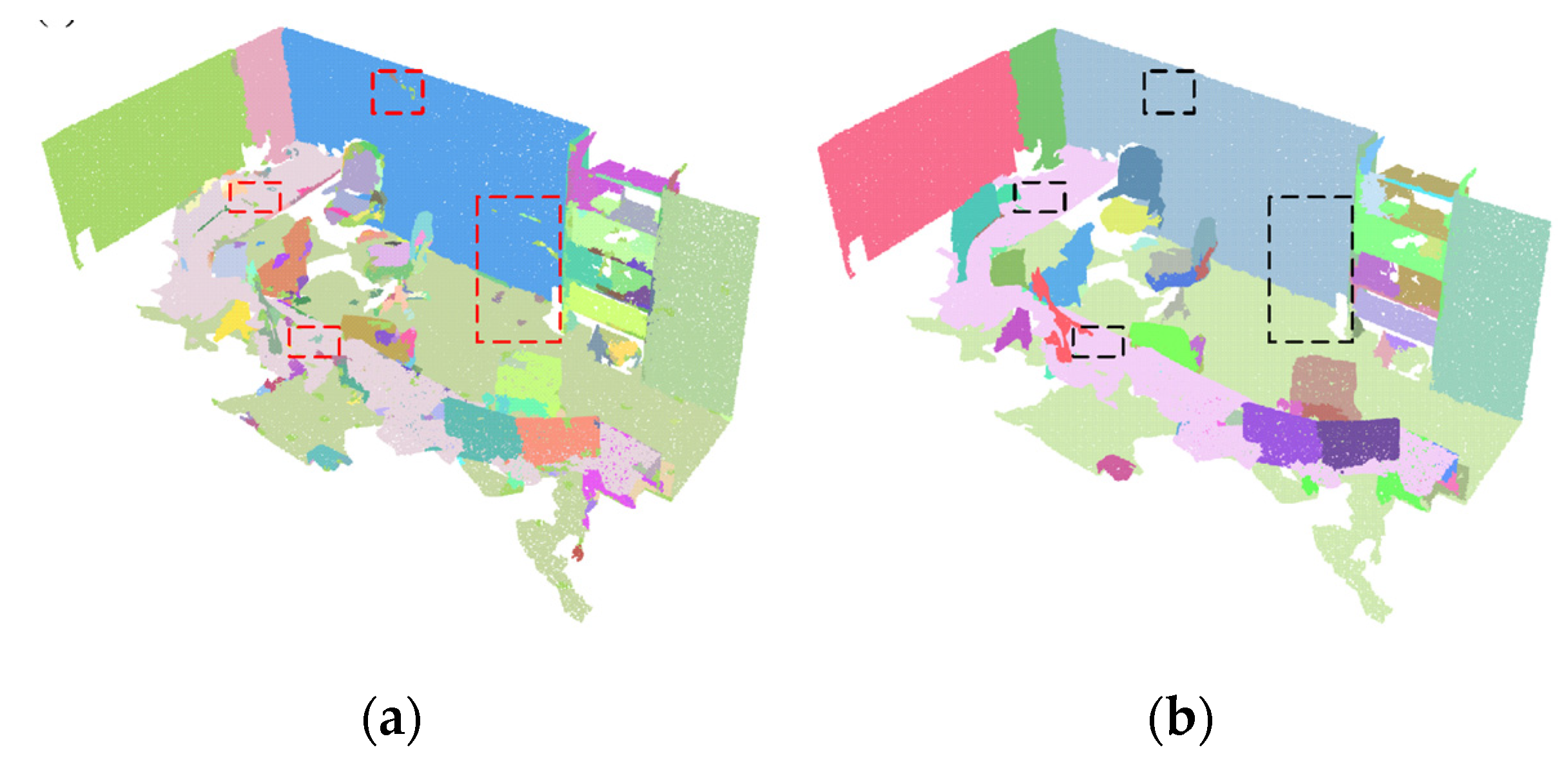
We need to merge these over-segmented parts into its neighboring segment with the greatest size. For each segment, we check whether it contains at least $n_{count}$ patches. If the size of the part partitioning is less than or equal to the filter size threshold $n_{count}$, we merge it with the neighboring segment with the maximum size of surface patches. Part merging will continue until there is no part partitioning with a size less than $n_{count}$ in the indoor scene. As shown in Figure 3a, the over-segmented parts in the red box are merged into their neighboring segments, as depicted in the black box in Figure 3b.

2.5.2. Noise Filtering

There are some noisy point clouds at the boundary in the scene, and the surface patches generated by these noise points are independent of the global supervoxel adjacent graph. Due to the fact that MCGC is based on the supervoxel adjacent graph, the surface patches to which these noise points belong will generate wrong part partitioning in the scene. The number of noise points is usually small. Therefore we set a noise threshold $n_{outlier}$ in the final segmentation result to check whether the number of point clouds of each segment is less than $n_{outlier}$, in which the labels of all point clouds are reset to the outliers.

3. Results

This section describes the details of the experiments, including the specifications of the benchmark dataset, the evaluation criteria, the parameter settings, the qualitative and quantitative evaluation of MCGC, and the effect analysis. The MCGC algorithm is implemented by point cloud Library. All experimental studies were executed on an Intel(R) Core(TM) i7-11390H @ 3.40 GHz processor with 16 GB RAM.

3.1. Datasets Description

The performance of MCGC was evaluated using two benchmark indoor datasets. One dataset is Stanford large-scale 3D Indoor Spaces (S3DIS) benchmark dataset [57] which collected RGB-D point clouds using cameras, as displayed in Figure 4a, Figure 5a and Figure 6a, and the other one is from University of Zurich (UZH) research dataset which contains 3D scanned point datasets using a 3D laser scanner, as displayed in Figure 7a and Figure 8a. The UZH dataset can be downloaded and used on the website https://www.ifi.uzh.ch/en/vmml/research/datasets.html (accessed on 26 October 2022). Generally, the S3DIS dataset is more challenging than the UZH dataset due to the fact that the point clouds collected by structured-light sensors contain a lower point location precision and higher level of noise, both of which provide significant difficulties for PCS.

The S3DIS dataset was obtained with different point position precisions, point densities, and levels of outliers and noise and captured via the Matterport Camera. It includes six large-scale indoor regions with a total of 695,878,620 points and comprises a variety of indoor scenes, including offices, conference rooms, pantries, copy rooms, lounges, and hallways. The UZH dataset contains the available 3D scanned point datasets acquired using a Faro Focus 3D laser range scanner by the Visualization and MultiMedia Lab at two locations of the University of Zürich and one of ETH Zürich. Each indoor scene consists of an ASCII PTX file with color (x, y, z, intensity, r, g, b).

Table 1. Descriptions of the data.

Data		Points	Area	Height	Density	From
			(m2)	(m)	(Points/m3)
S3DIS	conference	1,922,357	42.75	4.5	9993	Matterport
	office-1	759,861	16.8	2.7	16,752	Matterport
	office-2	2,145,926	40.7	2.8	18,831	Matterport
UZH	Room-L9	10,997,024	23.4	3	156,653	Laser
	Room-L80	10,843,388	22.75	3	158,877	Laser

shows the statistics for the indoor scene data used in the experiment.

3.2. Evaluation Metric

The performance of MCGC was evaluated based on six metrics widely used to evaluate the object classification [44,48,49]. The evaluation metrics include segment precision $\left(S_P\right)$ and segment recall $\left(S_R\right)$, segment F1-score $\left(S_{F1}\right)$, over-segmentation rate $\left(R_{OS}\right)$ and under-segmentation rate $\left(R_{US}\right)$.

The segment precision $\left(S_P\right)$ and the segment recall $\left(S_R\right)$ and segment F1-score $\left(S_{F1}\right)$ are respectively defined as follows:

$$S_P=\frac{N_C}{N_S}$$

(6)

$$S_R=\frac{N_C}{N_G}$$

(7)

$$S_{F1}=2\ast \frac{S_P\ast S_R}{S_P+S_R}$$

(8)

where $N_C$ indicates the number of correct part partitioning. As in previous studies [58], we consider a segment to be valid if it overlaps with the ground truth by more than 80%. $N_S$ and $N_G$ respectively represent the total number of parts in our segmentation result and the total number of segments in the ground truth.

The over-segmentation rate $\left(R_{OS}\right)$ is a measure of the percentage of the segments in the truth value overlapping with the actual multiple partitioned segments, and the part under-segmentation rate $\left(R_{US}\right)$ is formulated as the percentage of the segments in the truth value overlapping with the multiple corresponding segments, as Equations (9) and (10). $N_{OS}$ is the number of segments with over-segmentation, and $N_{US}$ is the number of segments with under-segmentation.

$$R_{OS}=\frac{N_{OS}}{N_G}$$

(9)

$$R_{US}=\frac{N_{US}}{N_S}$$

(10)

3.3. Parameter Settings

Table 2. Parameter settings of MCGC method.

Parameter	Descriptor	Value
$r_{voxel}$	The voxel resolution	0.01 m
$r_{seed}$	The seed resolution	0.07 m
$\delta$	The distance threshold of the outliers	0.03 m
$t{h}_{convexity}$	The threshold of local convexity constraint	8
$t{h}_{color}$	The threshold of color constraint	25
$n_{count}$	The maximum number of patches of the component to be merged	3
$n_{outlier}$	The maximum number points of the separated parts to be outliers	50

lists the parameter settings of the MCGC method. The experimental parameters in our algorithm are primarily generated from surface patch generation, global energy optimization, multi-constraint graph clustering, and the post-refinement step. There are two parameters in surface patch generation, that are $r_{voxel}$ and $r_{seed}$, indicating the voxel resolution and seed resolution of the surface patches. The resolution will affect the fineness of segmentation and we set $r_{voxel}=0.01$ and $r_{seed}=0.07$ according to experience. The energy optimization process includes one key parameter $\delta$ which indicates the distance threshold of the outliers. We set $\delta =0.03$ which meets conditions of the outlier distance threshold for all indoor scenes in the experiments. In the process of multi-constraint graph clustering, we set $t{h}_{convexity}=8$ to ensure the effective object partitioning by local convexity and $t{h}_{color}=25$ to further refine the partitioning of the details on the structural planes. The post-refinement step uses two parameters, $n_{count}$ and $n_{outlier}.$ The components with the number of patches less than $n_{count}$ will be merged into the maximum adjacent components. The separated parts with the number of points less than $n_{outlier}$ will be labeled as outliers and we set $n_{outlier}=50$ in our experiments.

3.4. Qualitative Evaluation

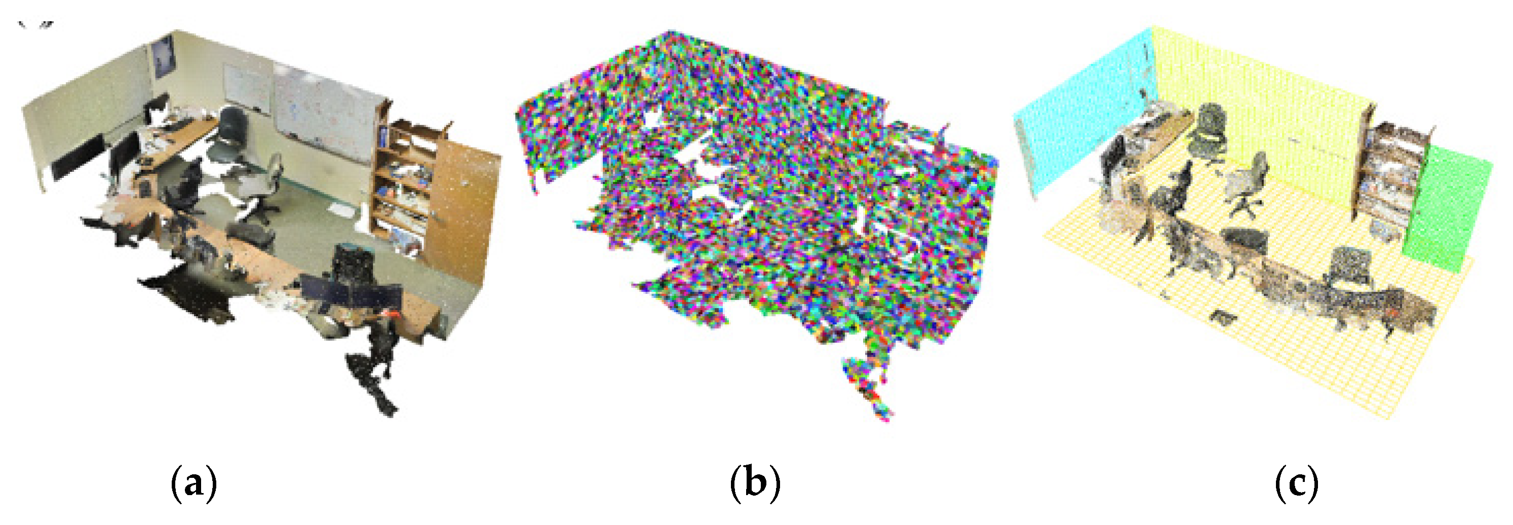
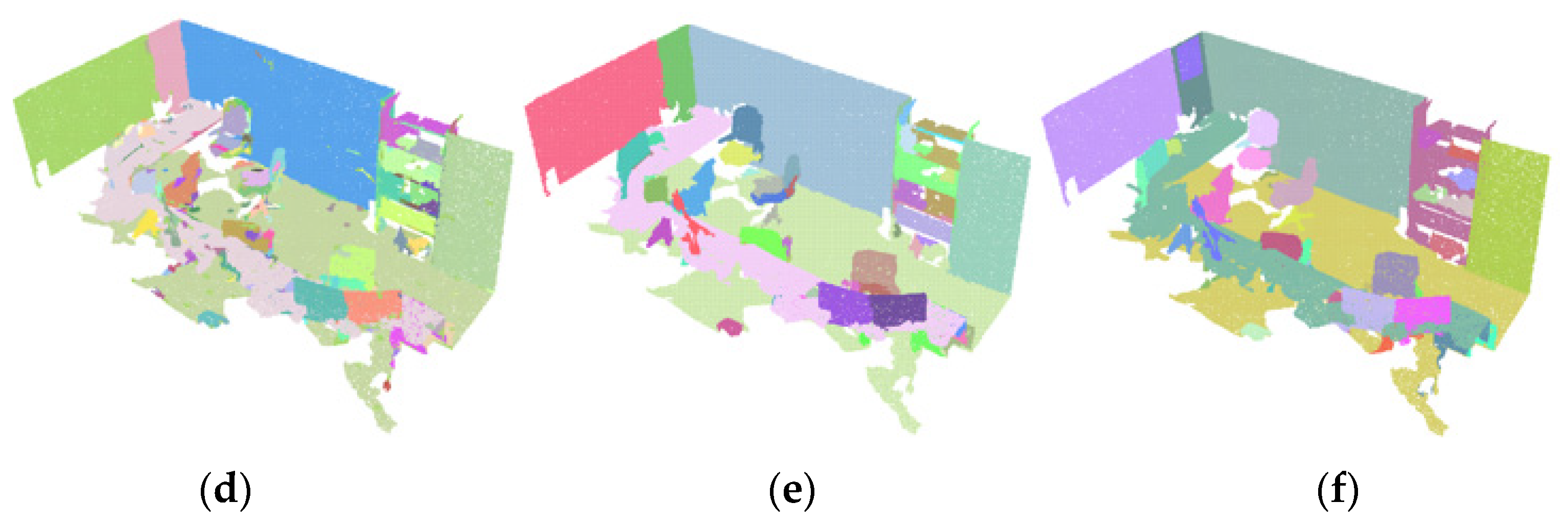
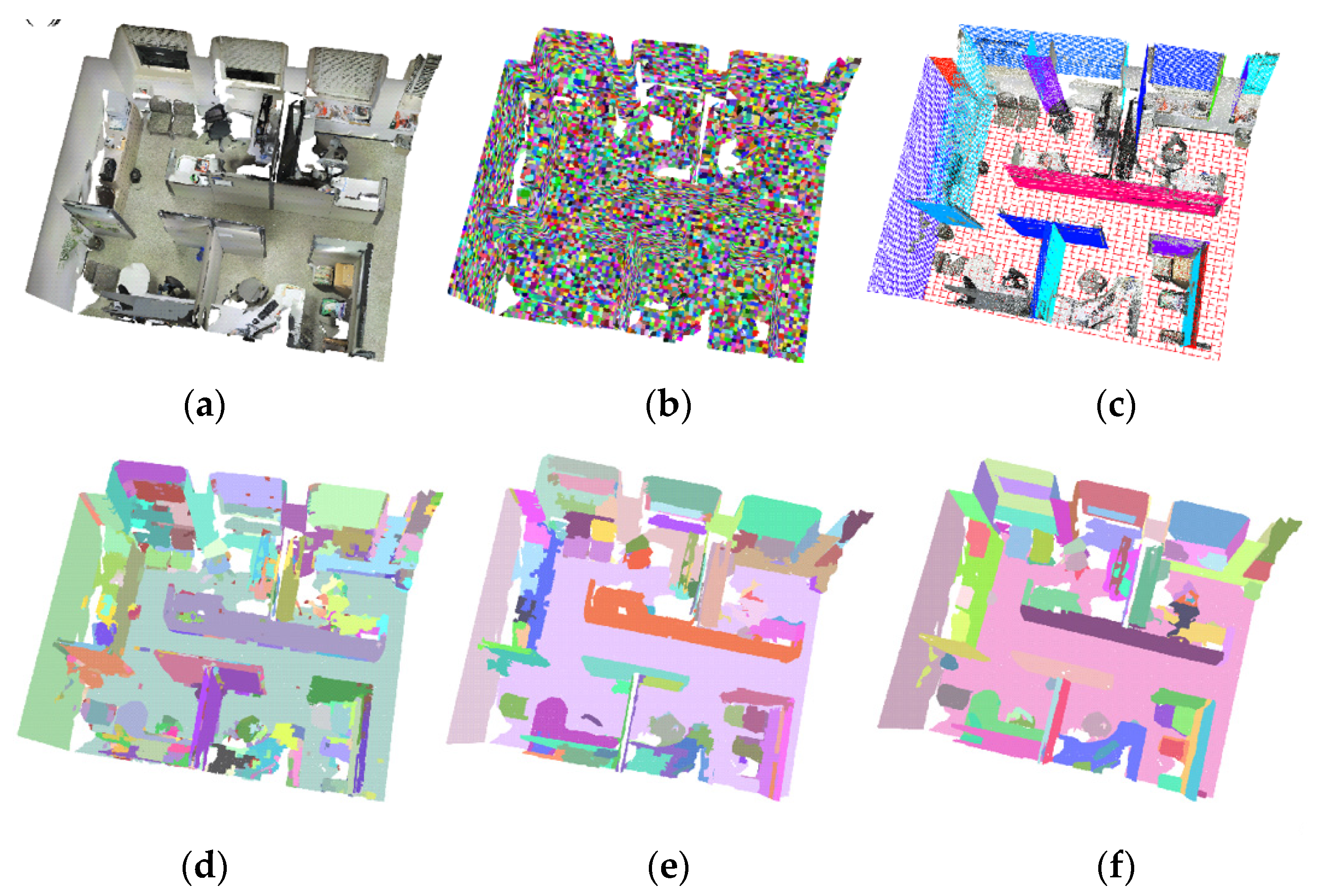
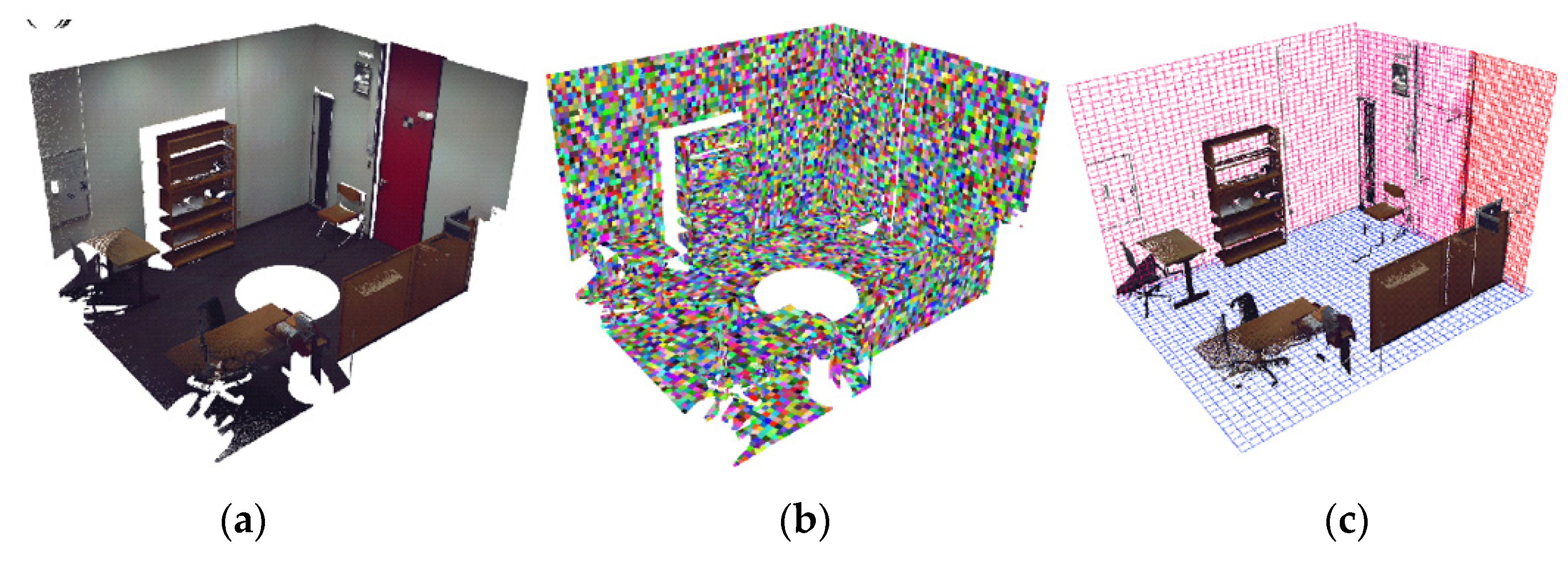
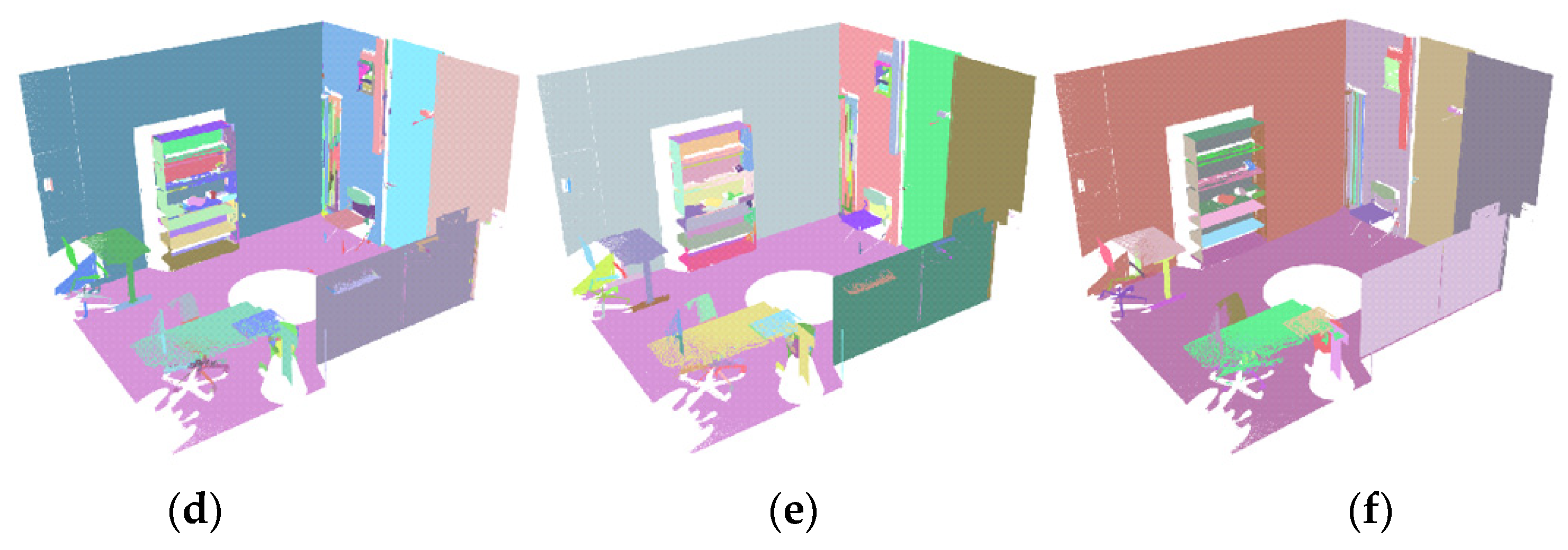
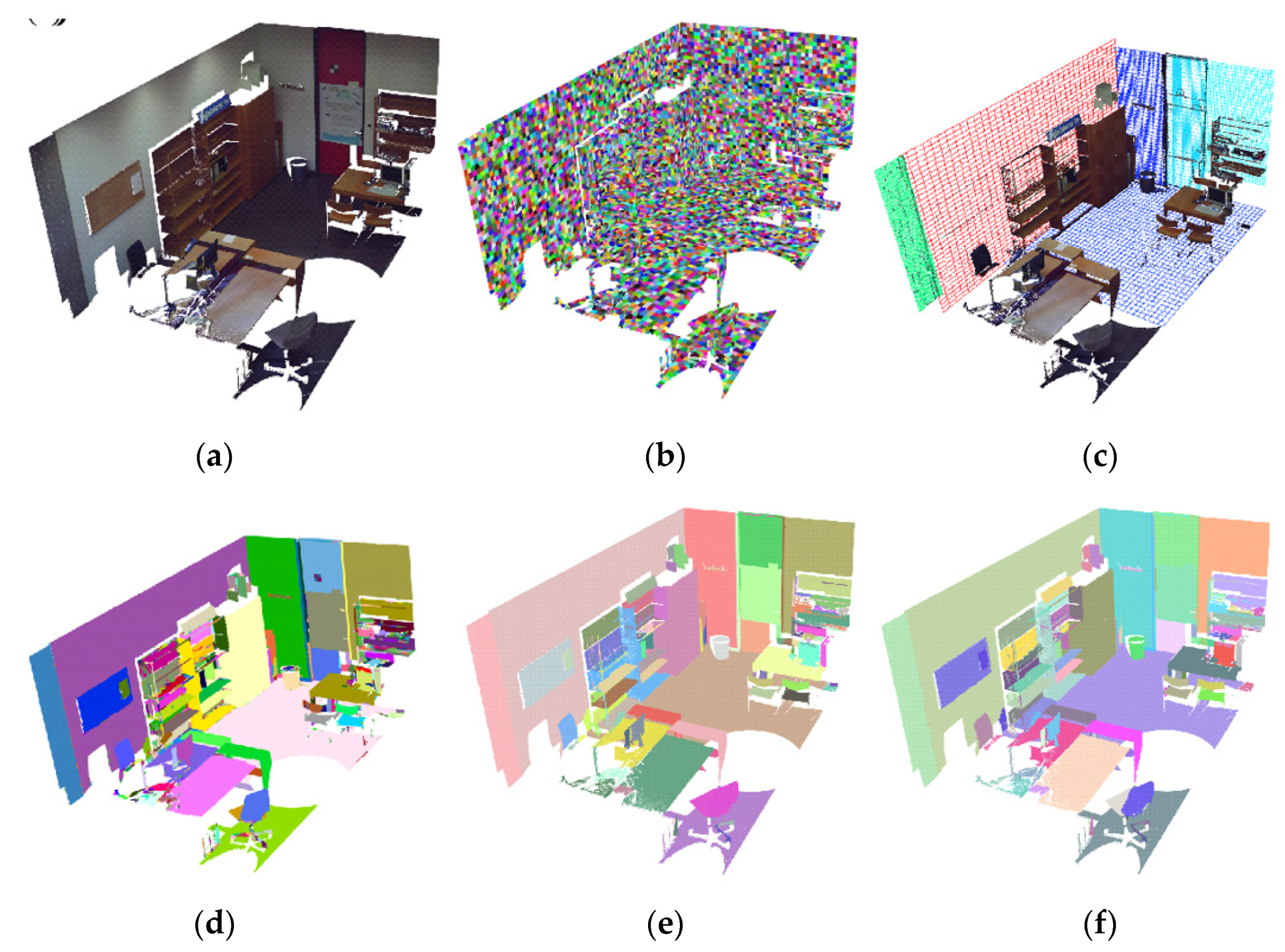
The MCGC method was tested both on the RGB-D benchmark dataset and the laser scanning benchmark dataset. Figure 4, Figure 5 and Figure 6 show the qualitative evaluation results on the S3DIS dataset, and Figure 7 and Figure 8 show the qualitative evaluation results on the UZH dataset. Figure 4a, Figure 5a, Figure 6a, Figure 7a and Figure 8a depict the raw point clouds, colored according to their RGB values. Figure 4b, Figure 5b, Figure 6b, Figure 7b and Figure 8b denote the over-segmented surface patches for input point clouds, where each patch is marked differently. Figure 4c, Figure 5c, Figure 6c, Figure 7c and Figure 8c show the structural plane extraction results, including the extracted scene structural planes and the remaining point clouds that are not used to fit the structural planes in the scene, where each plane is represented by a single color. Figure 4d, Figure 5d, Figure 6d, Figure 7d and Figure 8d display the indoor segmentation results after multi-constraint graph clustering and the final results after post-refinement are shown in Figure 4e, Figure 5e, Figure 6e, Figure 7e and Figure 8e, where each segment is dotted in a different color. Figure 4f, Figure 5f, Figure 6f, Figure 7f and Figure 8f show the ground truths which are manually labeled, where each segment is labeled in a different color.

For structural planes and objects above them, we segmented most structural planes correctly due to the accurately extracted planes from robust structure plane extraction and the correct match between patches and planes via global energy optimization. However, there are a few error cases in splitting the details above the walls, as exemplified by the whiteboards on the walls from the conference in Figure 4 and office-1 in Figure 5. The under-segmentation of the whiteboards is caused by the similarity of the colors between objects and walls. Consequently, as shown by the decorative paintings in Figure 4 and the windows in Figure 6, the objects whose colors differ significantly from the walls can be separated by color restraint. However, it is challenging to segment objects by similar colors to the walls, such as whiteboards.

For indoor objects, we detected most individual indoor objects by edge classifier based on the label assignment between patches and structural planes. Then, indoor objects can be further distinguished by the local convexity constraint. However, there are a few limitations in the local surface convexities. When the surface patches are at the boundary of the objects or the point cloud within the patch is noisy, the estimation of the normals of the patches will be inaccurate, resulting in incorrect classification of the local surface convexities, and subsequently leads to the object partitioning to fail, such as the undetected objects on the bookcase from the conference in Figure 4. Several pipes of the radiator in Figure 7 are over-segmentation for the same reason.

In general, most indoor structures, objects and/or their parts in the scenes, including walls, floors, windows, computers, backs of chairs, and legs of tables, can be correctly separated by our method. The qualitative results indicate that MCGC achieved a satisfactory performance of indoor PCS both in a high-precision laser scanning dataset and a low-quality RGB-D point cloud dataset.

3.5. Quantitative Evaluation

In order to evaluate the performance of MCGC for indoor PCS in a more rigorous statistical manner, we conducted a quantitative analysis using the five metrics mentioned in Section 3.2 and counted the execution time of each procedure of the experiment.

Table 3. Quantitative results of 3D indoor segmentation.

Data	${\mathit{S}}_{\mathit{P}}$ (%)	${\mathit{S}}_{\mathit{R}}$ (%)	${\mathit{R}}_{\mathit{O}\mathit{S}}$ (%)	${\mathit{R}}_{\mathit{U}\mathit{S}}$ (%)	${\mathit{S}}_{\mathit{F}1}$ (%)
Conference	73.53	69.44	8.30	10.29	71.43
Office-1	70.91	72.22	9.26	7.27	71.56
Office-2	79.45	66.67	10.34	8.22	72.50
Room-L9	77.05	87.04	11.11	3.28	81.74
Room-L80	74.26	80.65	4.30	2.97	77.32

reports the quantitative results of the five metrics on the experimental data. The results demonstrated in Table 3 indicate that MCGC provides high performance in the partitioning of the whole indoor scenes into object parts with $S_P$ and $S_{F1}$, above 0.7 both on the RGB-D point cloud dataset and the laser scanning dataset. The execution time data in

Table 4. Execution time of experimental data.

Data	Computing Time (s)
	Surface Patch Generation	Robust Structural Plane Extraction	Patch-to-Plane Assignment	Multi-Constraint Graph Clustering	Post-Refinement	Total Time
Conference	0.762	3.04	0.002	0.17	0.266	4.24
Office-1	0.291	1.092	0.002	0.052	0.146	1.583
Office-2	0.646	5.26	0.001	0.292	0.425	6.624
Room-L9	4.656	17.685	0.002	0.316	0.885	23.544
Room-L80	2.692	10.08	0.002	0.222	0.536	13.532

shows that the MCGC can quickly process scene point clouds, further validating the effectiveness of the MCGC.

For the S3DIS dataset, the $S_P$, $S_R$ and $S_{F1}$ are all above 0.7 and the $R_{OS}$ and $R_{US}$ are below 0.1 in the results of office-1, validating the feasibility of the MCGC. The $R_{US}$ of 7.27% mainly came from the unrecognized whiteboard on the wall and small objects on the bookshelf, as shown in Figure 6. The $R_{OS}$ of 9.26% is mainly due to incorrect local convex edge classification caused by the noise on the curved surface of the office chairs. In office-2, which contains more complicated details compared with the office-1, the $S_P$ of office-2 is higher than the former, but the $S_R$ is slightly underperforming. The same reason as office-1 caused the errors. In the conference, the under-segmentation rate of the conference was 10.29%. The errors were caused by missing some object partitioning on the bookshelf, as shown in Figure 5. Due to the occlusion between the bookshelves, the estimated normals of the noisy point clouds are incorrect, subsequently resulting in the small objects cannot be separated by local surface convexities.

For the UZH dataset, the $S_{F1}$ is improved and the $R_{OS}$ is reduced compared with the S3DIS dataset since the noise level of point clouds scanned by laser is lower than that collected by structured-light sensors, which improves the overall segmentation accuracy. The $S_R$ and the $S_{F1}$ of Room-L9 reaches 87.04 and 81.74, achieving satisfactory segmentation results. However, the $R_{OS}$ of 11.11% is mainly due to holes caused by occlusion in scanned point clouds. Missed point clouds caused discontinuities of geometric properties, leading to over segmentation. The $R_{US}$ and $R_{OS}$ of Room-L80 is lower than the former since the point clouds collected in Room-L80 is more complete with less occlusion and missing data, reaching high precision scene PCS with the $S_R$ of 80.65, the $S_P$ of 74.26 and the $S_{F1}$ of 77.32.

The execution time of each procedure of the MCGC algorithm is listed in Table 4. The time taken for multi-constraint graph clustering and post-refinement is just 10% of the overall time cost. It can be found that robust structural plane extraction consumes on average 70% of the overall time and the time spent on the remaining stages is insignificant. The overall time cost is calculated and listed in the last column of Table 4. The average time achieved to process 1 million points is about 1.38 s (724,000 points per second) by running our proposed method. Total processing time is dependent on the number of initial point clouds and proportional to the complexity of the scene data. This reflects the time-efficient advantage of MCGC, which is able to process large-quantity point clouds of scenes in real time.

In summary, we evaluated the MCGC on indoor scenes consisting of a variety of indoor structures and indoor objects in various shapes. The quantitative evaluation results demonstrate that our method achieves high performance in both accuracy and time efficiency for different indoor datasets collected by different sensors.

3.6. Effect Analysis

To further investigate the effects of our contribution on indoor PCS, we also calculate the metrics of MCGC-1, MCGC-2, MCGC-3, MCGC-4, and MCGC-5, which are the variants of the MCGC method.

First, we evaluated the performance of indoor PCS using only local convex constraints, denoted as MCGC-1. Based on the MCGC-1, we added the procedure of global robust structural plane extraction described in Section 2.2. As such, the effectiveness of the global plane constraint and the local geometric constraint joining together for indoor PCS can be quantitatively evaluated, denoted as MCGC-2. According to the corresponding metrics listed in

Table 5. Performance analysis of the MCGC.

Data		${\mathit{S}}_{\mathit{P}}$ (%)	${\mathit{S}}_{\mathit{R}}$ (%)	${\mathit{R}}_{\mathit{O}\mathit{S}}$ (%)	${\mathit{R}}_{\mathit{U}\mathit{S}}$ (%)	${\mathit{S}}_{\mathit{F}1}$ (%)
Room_L80	MCGC-1	39.67	51.61	13.98	7.44	44.86
	MCGC-2	46.09	56.99	16.13	5.22	50.96
	MCGC-3	52.73	62.37	21.51	0.9	57.15
	MCGC-4	71.43	75.27	4.3	6.1	73.28
	MCGC-5	50.45	60.22	16.13	2.7	54.9
	MCGC	74.26	80.65	4.3	2.97	77.32
Conference	MCGC-1	30.95	31.33	3.61	8.33	31.13
	MCGC-2	36.84	42.17	16.87	9.47	39.32
	MCGC-3	48.84	50.6	12.05	2.33	49.71
	MCGC-4	68.57	57.83	7.23	12.86	62.75
	MCGC-5	39.58	45.78	10.84	7.29	42.46
	MCGC	73.53	69.44	8.3	10.29	71.43

, MCGC-2 increased the $S_P$, $S_R$ and $S_{F1}$ on the selected two point clouds compared with MCGC-1, which indicates that it is effective in joining the global plane constraint and the local geometric constraint together for indoor PCS.

To further accurately evaluate the effect of our innovation, we evaluated the case in which structural plane extraction was not included. In other words, we used the plane results in the phase of scene plane detection described in Section 2.2.1 for subsequent experiments, and did not use prior knowledge to extract the structural planes described in Section 2.2.2. In this regard, we can accurately evaluate whether the design of structural plane extraction is effective in the procedure of the robust structural plane extraction, denoted as MCGC-3. As shown in Table 5, MCGC far surpassed MCGC-3 in terms of the $S_P$, $S_R$ and $S_{F1}$, which demonstrates the structural plane extraction process after the scene plane detection process can significantly improve the precision of indoor PCS. All detected planes in the scene that participated in the segmentation will cause error cases of the object over segmentation with the increased $R_{OS}$ from (4.3 and 8.3) to (21.51 and 12.05).

Next, we evaluated the case in which the color constraint was not included in the MCGC, denoted as MCGC-4. By comparing the metrics of MCGC-4 and MCGC in Table 5, it can be seen that the color constraint plays a part in improving the efficiency of indoor PCS. In this case, the objects on the structural planes can not be effectively distinguished, such as posters and blackboards, resulting in an increase in the $R_{US}$.

Finally, we evaluated the case in which the procedure of post-refinement was not included in the MCGC, denoted as MCGC-5. According to the corresponding metrics listed in Table 5, the $S_P$, $S_R$ and $S_{F1}$ of MCGC-5 is greatly reduced without the post-refinement procedure, which indicates that the post-refinement procedure enhances the capability of filtering the wrong segments caused by the outliers, with the decreased $R_{OS}$ from (16.13 and 10.84) to (4.3 and 8.3).

4. Discussion

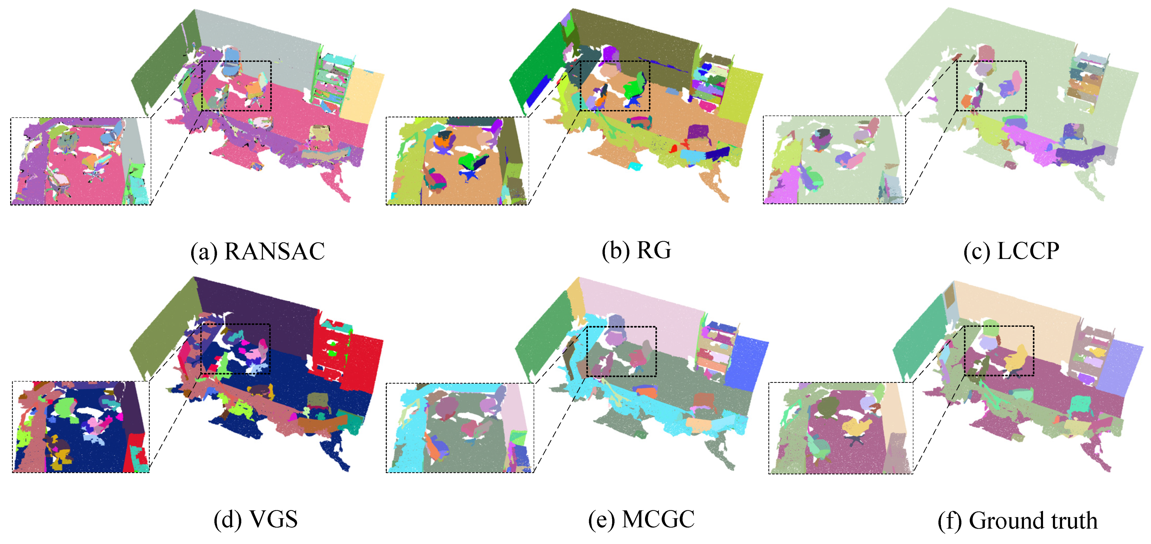
We further analyzed and discussed the effectiveness of the MCGC compared with the state-of-the-art segmentation algorithms with the same datasets. Efficient RANSAC [11] is the most widely used and cited method for detecting 3D shapes, and it has been proven useful for scene segmentation. Rabbani et al. [59] proposed a region growing (RG) method with better performance than the classic PBRG method. S. Stein et al. [51] proposed a recent object partitioning method using local convexity, denoted as LCCP. Xu et al. [44] proposed a voxel-based method for building structure segmentation using a probabilistic model. As a result, these most advanced algorithms of PCS are adopted as a performance comparison benchmark. The key parameters of these methods are set according to the parameters suggested in the original papers. Figure 9, Figure 10, Figure 11, Figure 12 and Figure 13 show the comparison visualization results and the corresponding evaluation metrics and execution time are listed in

Table 6. Performance comparison of indoor segmentation with different methods.

Data	Method	${\mathit{S}}_{\mathit{P}}$ (%)	${\mathit{S}}_{\mathit{R}}$ (%)	${\mathit{R}}_{\mathit{O}\mathit{S}}$ (%)	${\mathit{R}}_{\mathit{U}\mathit{S}}$ (%)	${\mathit{S}}_{\mathit{F}1}$ (%)	Runtime (s)
Conference	Efficient RANSAC	19.35	28.92	48.19	7.50	23.19	6.3027
	RG	32.94	33.73	21.69	12.94	33.33	20.43
	LCCP	30.95	31.33	3.61	8.33	31.13	3.47
	VGS	42.86	43.37	28.92	7.14	43.12	10.101
	MCGC	73.53	69.44	8.30	10.29	71.43	5.771
Office-1	Efficient RANSAC	19.82	40.74	42.59	2.70	26.67	3.846
	RG	50.00	46.30	20.37	6.00	48.10	8.352
	LCCP	31.58	44.44	9.26	10.53	36.92	1.497
	VGS	53.66	40.72	16.67	14.63	46.31	4.752
	MCGC	70.91	72.22	9.26	7.27	71.56	2.586
Office-2	Efficient RANSAC	40.23	39.77	34.48	10.23	40.00	10.138
	RG	20.96	40.23	43.68	3.00	27.55	78.094
	LCCP	28.21	25.29	16.09	11.54	26.67	4.486
	VGS	33.58	45.98	36.78	7.46	38.81	9.786
	MCGC	79.45	66.67	10.34	8.22	72.50	6.88
Room-L9	Efficient RANSAC	24.36	35.19	27.78	6.41	28.83	78.450
	RG	34.44	57.41	35.19	5.56	43.05	266.326
	LCCP	27.06	42.59	11.11	10.59	33.09	37.638
	VGS	65.79	46.30	9.26	10.53	54.35	46.630
	MCGC	77.05	87.04	11.11	3.28	81.74	23.544
Room-L80	Efficient RANSAC	47.62	43.00	16.13	11.90	45.16	64.287
	RG	42.22	61.29	9.70	2.96	50.00	155.026
	LCCP	39.67	51.61	13.98	7.44	44.86	24.788
	VGS	64.81	37.63	9.68	14.81	47.62	33.186
	MCGC	74.26	80.65	4.30	2.97	77.32	13.532

. The results show that the MCGC method is superior to other benchmark methods. More specifically, some conclusions can be drawn from the comparison results.

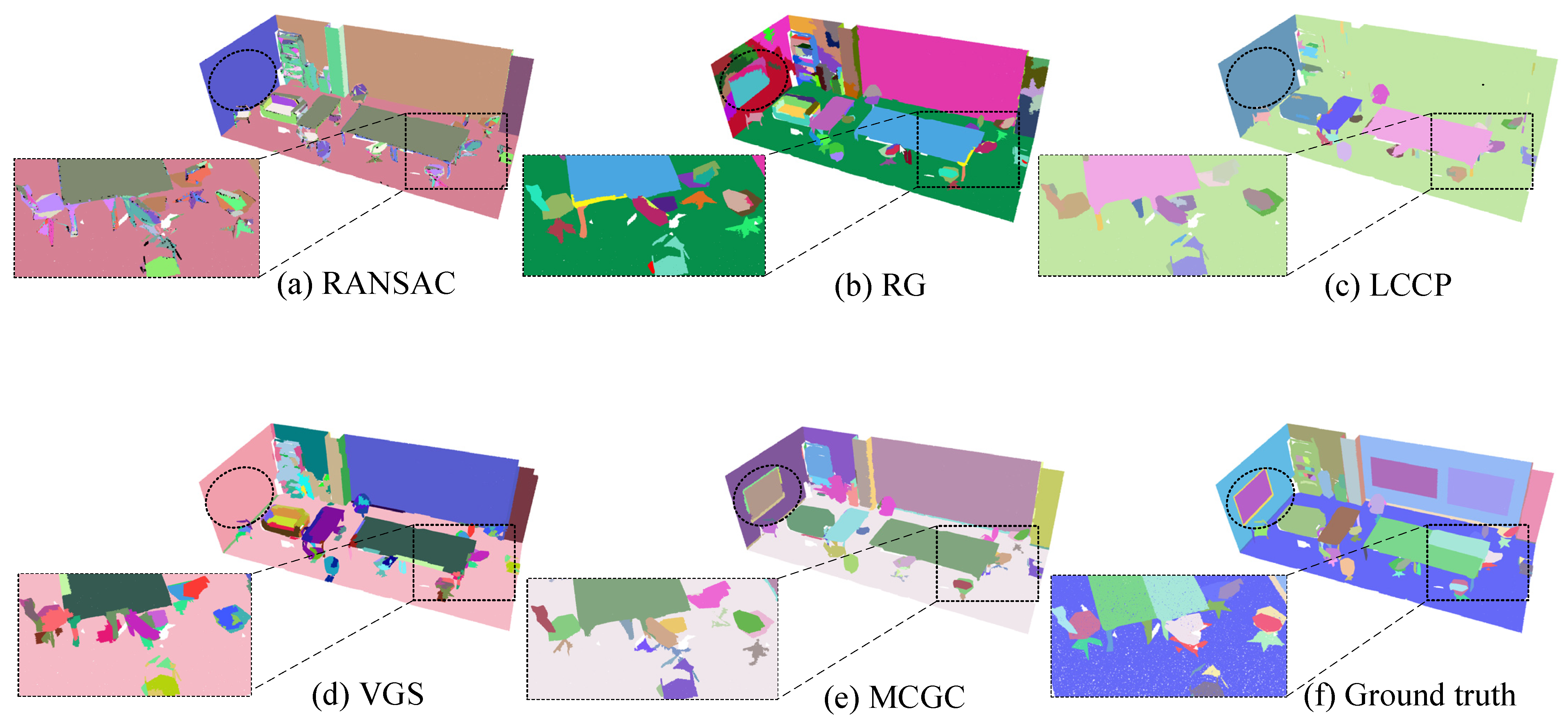
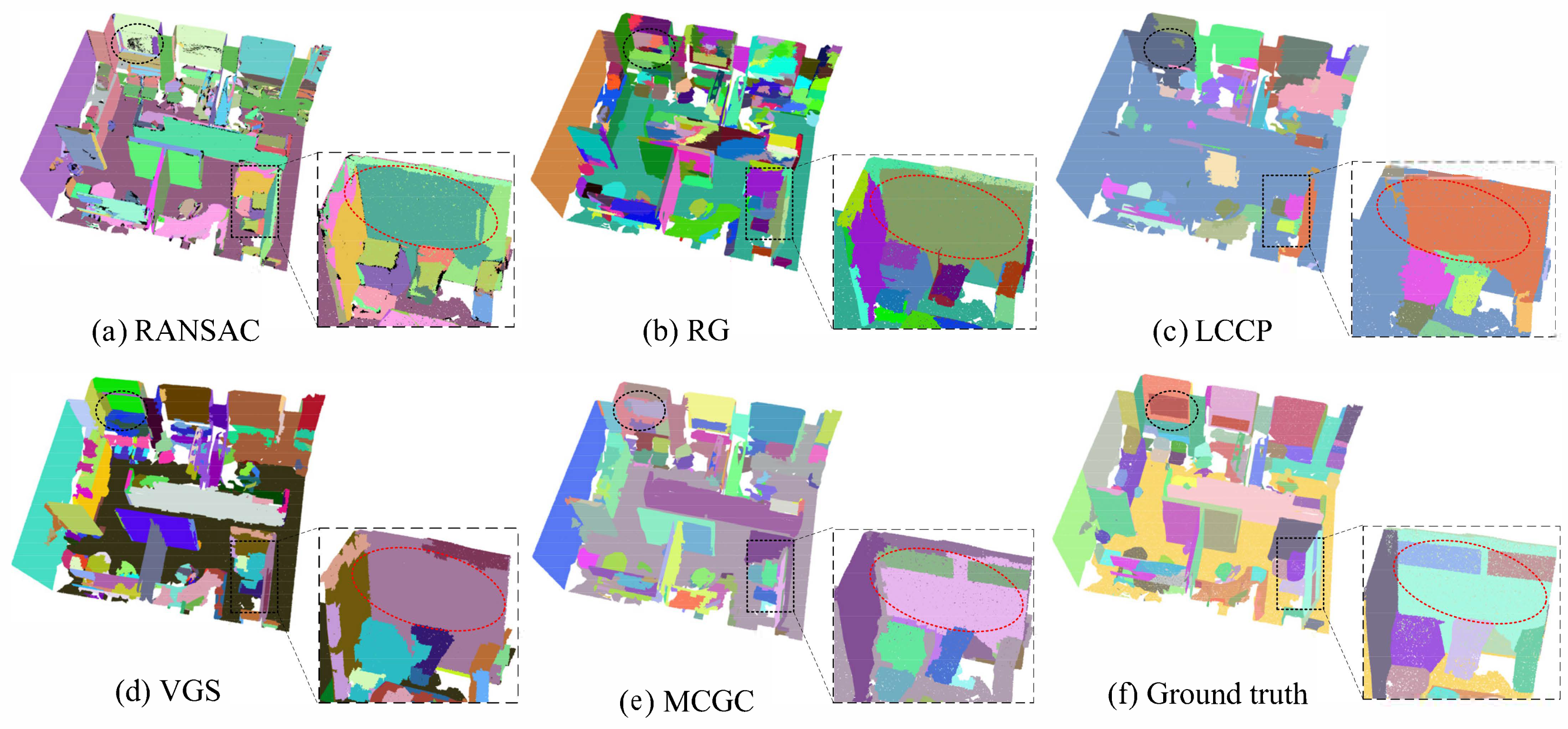
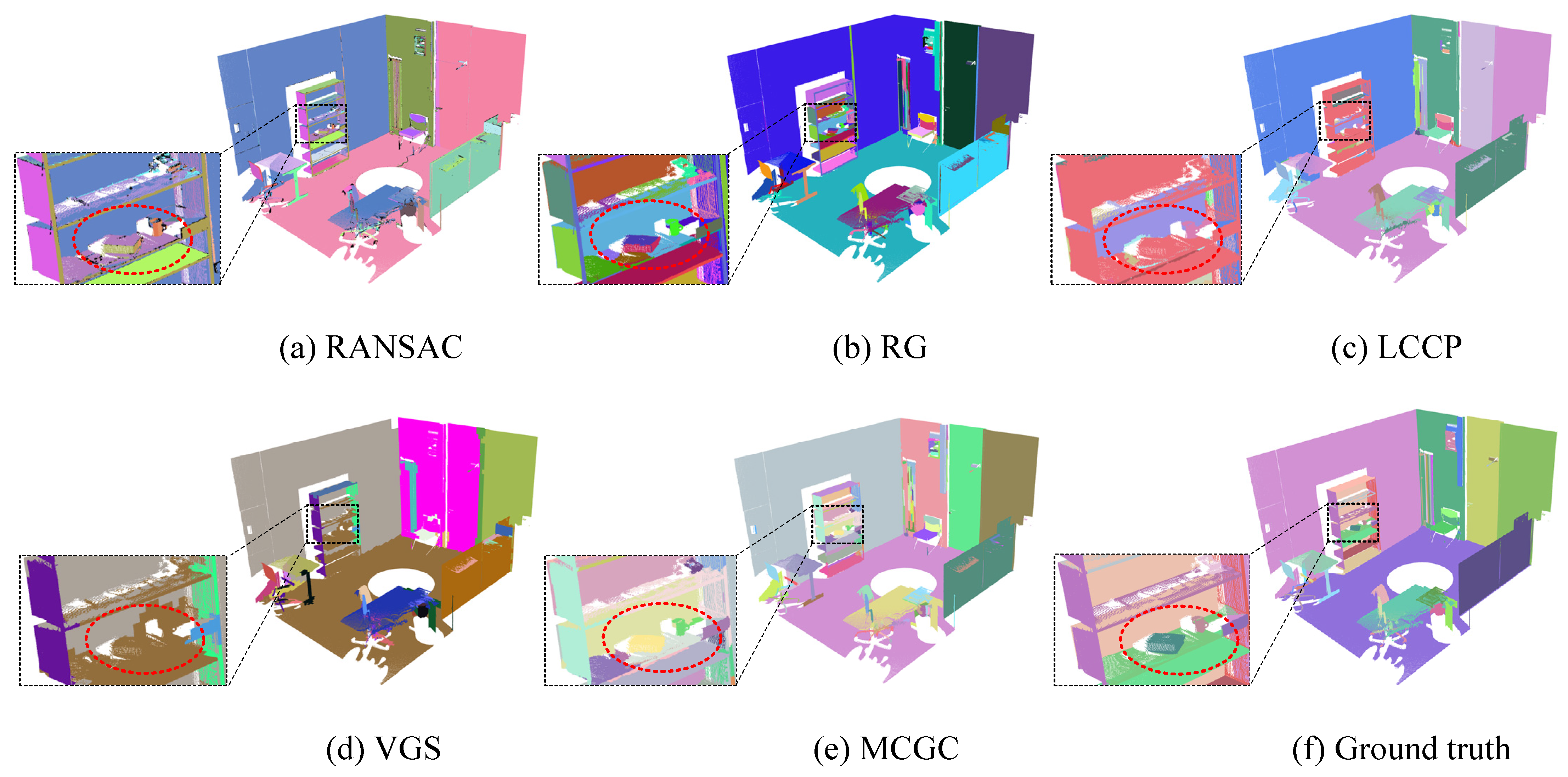
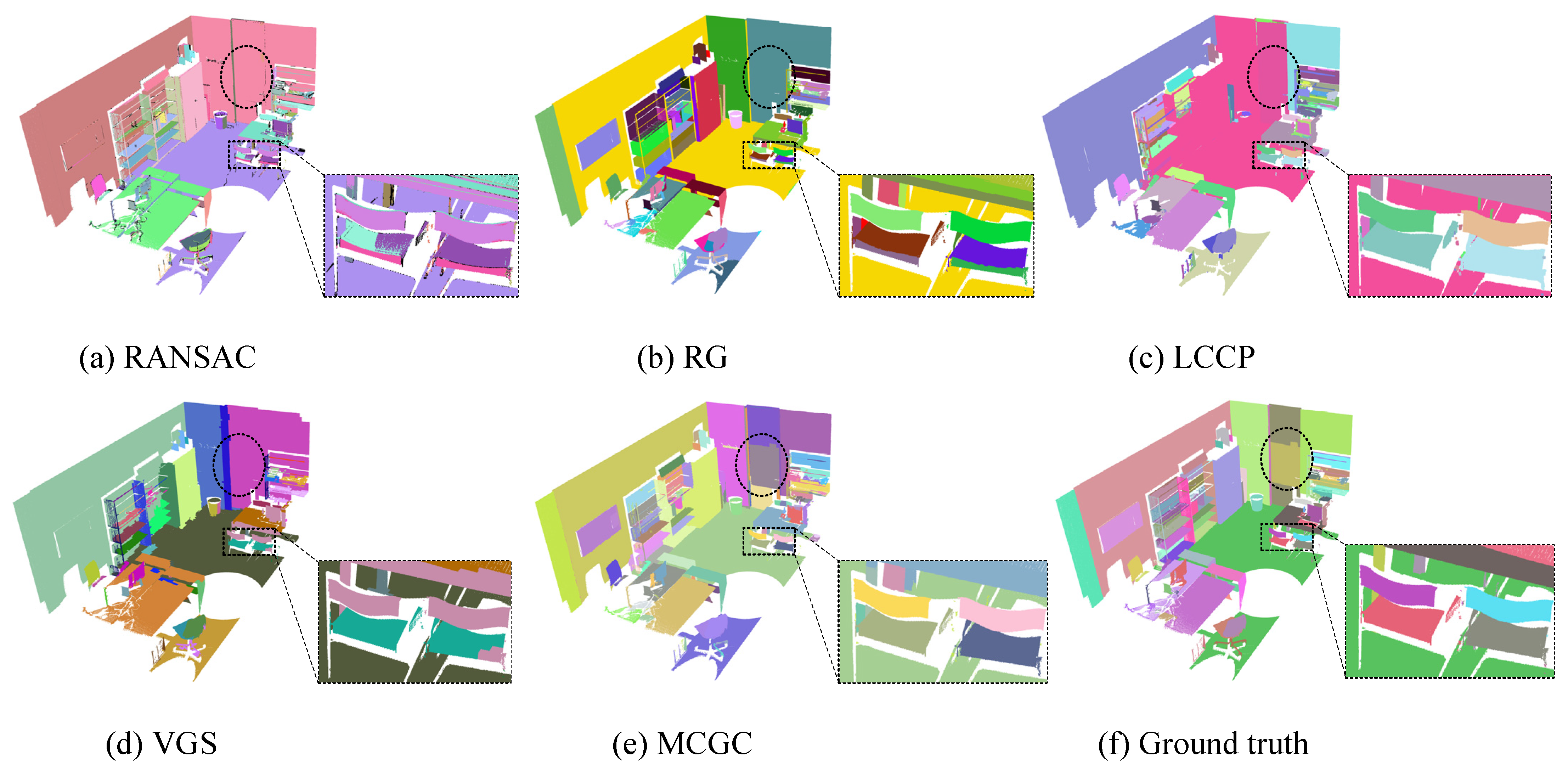
Figure 9a, Figure 10a, Figure 11a, Figure 12a and Figure 13a and Figure 9b, Figure 10b, Figure 11b, Figure 12b and Figure 13b demonstrate that when the local optimal algorithms (RANSAC and RG methods) are used to segment an indoor scene, the segmentation results are highly scattered and many object parts are over-segmented. In addition, the quantitative results presented in Table 6 indicate that RG and RANSAC obtain relatively lower $S_P$, $S_R$ and $S_{F1}$ values, especially higher $R_{OS}$ than the MCGC. In the following discussion, we analyze the factors that contributed to the lower performance.

RG method merges neighboring points that satisfy the smooth constraint based on the angle difference between the normals of points, which is appropriate for detecting planes with small normal differences, leading to the objects with curved surface structures in the indoor scene not being accurately separated, such as the over-segmented chair back in Figure 9b and Figure 10b. As the segmentation result is significantly affected by the differences between normals, the RG algorithm not only easily leads to the over-segmentation of indoor objects, such as the walls in Figure 11b, is but also difficult to split parts with small differences between normals, such as the whiteboards on the wall in Figure 9b and Figure 10b. It is noteworthy that the segmentation performance of the RG method on the UZH is significantly improved. As shown in the Room_L80 of Table 6, the $S_R$ of 61.29, the $S_{F1}$ of 50.00 and the $S_P$ of 42.22 overtake the RANSAC, LCCP and VGS method due to the lower level of noise and higher point position precision in the laser scanned dataset. In this regard, we can conclude that the RG method is very sensitive to the noise. However, the evaluation results of the MCGC method in the two datasets differ little due to statistical analysis based plane detection procedure which is robust to noise.

Detecting the primitives one by one is limited to the shape prior provided by RANSAC, extracting only five categories of primitives: plane, sphere, cylinder, cone, and ring. However, indoor objects are usually more complex geometric models with irregular shapes. Therefore, direct fitting of the models will lead to the problem of model mismatch and a higher over-segmentation rate. Moreover, greedy search for most inlier points often leads to the suboptimal solution with the transition error of the fitting models, which leads to the inaccurate boundaries between the object parts, such as the chair backs in Figure 9a. The details of objects are partitioned into many irregular parts, such as the cushion and foot of the chairs as shown in Figure 10a. To solve the limitations of local optimal algorithms mentioned above, MCGC not only uses global optimization to achieve robust segmentation of high-level noise and clutter data sets, but also uses local convexity information and color constraint to complete the segmentation of various indoor objects and the details on the indoor structures.

The LCCP method performed better on the issue of over-segmentation than RANSAC and RG, as shown in $R_{OS}$ from Table 6, due to the object partitioning separated by local surface convexities. Compared with LCCP, the MCGC has better performance in $S_P$, $S_R$ and $S_{F1}$ values. From the visualization results, it can be found that the LCCP algorithm fails to split the structural walls and floors from the scene, and also fails to separate isolated objects, such as the tables in Figure 11c. The former is because the normals of the adjacent patches are very similar, and they fail to meet the singular value threshold set in LCCP for compensating the sensor noise, resulting in the errors of the object partitioning. The latter is because the LCCP algorithm fails to form a closed loop over convex edges during the region growing process. It can be seen that there are many small segments on the edges of walls that are not connected successfully, as shown in Figure 10c. To sum up, the constraint range of geometric convexity measure in LCCP algorithm is finite, and it is difficult to achieve the segmentation of planar large-scale structural parts and curved objects only by a single geometric convexity measure at the same time in dense indoor scenes.

The VGS method constructed an adjacency graph between the voxels, which is similar to the MCGC method we proposed. The main difference is the criterion to split the edges in the graph. Specifically, the VGS method uses the surface connectivity, the shape similarity, and the spatial distance to calculate the saliencies of the weighted edges, while the MCGC method considers the structural planes of indoor scenes, local convexity and color of point clouds to divide the graph into several subgraphs. By comparing the visualization results of Figure 9d–f, it can be found that the red wall beside the bookcase is not separated from the bookcase which are accurately separated in the MCGC method. Similar cases appear in the Figure 12d and Figure 13d since the large structural planes in the scene are not easy to distinguish by local geometric attributes, leading the $R_{US}$ of the VGS method is higher compared with others. Nevertheless, the overall segmentation performance is better than the RANSAC, RG and LCCP method with higher $S_P$, $S_R$ and $S_{F1}$.

The execution time listed in Table 6 shows that compared with RANSAC and RG, the execution time of the MCGC is reduced by two orders of magnitude, which indicates that surface patch generation significantly accelerates computation speed and reduces calculation cost. In summary, the experiment results show that the MCGC method greatly outperforms the efficient RANSAC, RG, LCCP, VGS methods.

The MCGC we proposed respectively deal with the main structural planes and attached objects (walls, floors, windows, skirting lines, decorative paintings, etc.) and the indoor objects (sofas, desks, bookcases and chairs, etc.). The workflow for respectively processing indoor parts with different geometric attributes enhances the ability of the partitioning of cluttered indoor scenes into object parts with more details, improving the accuracy and completeness of indoor segmentation. However, the MCGC method has limitations in handling spatially discontinuous objects. Compared with Figure 12f, the dark green door with a poster on it is partitioned into two pieces with the poster between them displayed in Figure 12e. The two pieces of the door divided by the poster belong to an indoor object in theory, but the algorithm fails to segment such spatially discontinuous objects. The same error cases occur when there are occlusions, holes or missing data caused by limitations of acquisition devices. In future work, we will further utilize global information to overcome these limitations. Specifically, global semantic information will participate in the segmentation algorithm together with local geometric properties.

5. Conclusions

• This paper introduced a novel method (MCGC) based on multi-constraint graph clustering for indoor segmentation, which effectively exploits pluralistic information of 3D indoor scenes. Importantly, we closely integrated extracted structural planes, local surface convexity, and color information of objects for scene segmentation to solve the issues of the model mismatch and the lack of detailed parts in the previous unsupervised segmentation algorithms. In particular, we presented a robust plane extraction method and used global optimization to assign patches to the indoor structural planes. Moreover, we demonstrated how the extracted planes are jointly segmented with local convexity information and color constraint by employing a graph clustering method. In addition, the entire MCGC algorithm is based on surface patches generated from the point cloud, and a post-refinement step is designed to filter the outliers, which significantly improves computation speed and saves computation overhead. The segment precision and recall of experimental results reach 70% on average, at an average processing speed of 724,000 points per second.

The results of the experiment on the challenging RGB-D point cloud dataset (S3DIS) and the laser scanned dataset (UZH) show that the MCGC greatly enhances the efficiency and the accuracy of the indoor PCS and outperforms the state-of-the-art unsupervised scene segmentation methods. In planned future work, we will consider improving the boundary accuracy of the object partitioning and explore better segmentation criteria to effectively segment indoor scenes.

References

1. Zhao, B.; Hua, X.; Yu, K.; Xuan, W.; Chen, X.; Tao, W. Indoor Point Cloud Segmentation Using Iterative Gaussian Mapping and Improved Model Fitting. IEEE Trans. Geosci. Remote Sens. 2020, 58, 7890–7907. [Google Scholar] [CrossRef]
2. Macher, H.; Landes, T.; Grussenmeyer, P. From Point Clouds to Building Information Models: 3D Semi-Automatic Reconstruction of Indoors of Existing Buildings. Appl. Sci. 2017, 7, 1030. [Google Scholar] [CrossRef] [Green Version]
3. Biglia, A.; Zaman, S.; Gay, P.; Aimonino, D.R.; Comba, L. 3D point cloud density-based segmentation for vine rows detection and localisation. Comput. Electron. Agric. 2022, 199, 107166. [Google Scholar] [CrossRef]
4. Maturana, D.; Scherer, S. VoxNet: A 3D Convolutional Neural Network for real-time object recognition. In Proceedings of the 2015 IEEE/RSJ International Conference on Intelligent Robots and Systems (IROS), Hamburg, Germany, 28 September–2 October 2015; pp. 922–928. [Google Scholar] [CrossRef]
5. Chen, X.; Wu, H.; Lichti, D.; Han, X.; Ban, Y.; Li, P.; Deng, H. Extraction of indoor objects based on the exponential function density clustering model. Inf. Sci. 2022, 607, 1111–1135. [Google Scholar] [CrossRef]
6. Xu, Z.; Liang, Y.; Xu, Y.; Fang, Z.; Stilla, U. Geometric Modeling and Surface-Quality Inspection of Prefabricated Concrete Components Using Sliced Point Clouds. J. Constr. Eng. Manag. 2022, 148, 04022087. [Google Scholar] [CrossRef]
7. Park, J.; Kim, J.; Lee, D.; Jeong, K.; Lee, J.; Kim, H.; Hong, T. Deep Learning–Based Automation of Scan-to-BIM with Modeling Objects from Occluded Point Clouds. J. Manag. Eng. 2022, 38, 04022025. [Google Scholar] [CrossRef]
8. Fan, Y.; Wang, M.; Geng, N.; He, D.; Chang, J.; Zhang, J.J. A self-adaptive segmentation method for a point cloud. Vis. Comput. 2017, 34, 659–673. [Google Scholar] [CrossRef]
9. Wu, H.; Zhang, X.; Shi, W.; Song, S.; Tristan, A.C.; Li, K. An Accurate and Robust Region-Growing Algorithm for Plane Segmentation of TLS Point Clouds Using a Multiscale Tensor Voting Method. IEEE J. Sel. Top. Appl. Earth Obs. Remote Sens. 2019, 12, 4160–4168. [Google Scholar] [CrossRef]
10. Saglam, A.; Makineci, H.B.; Baykan, N.A.; Baykan, K. Boundary constrained voxel segmentation for 3D point clouds using local geometric differences. Expert Syst. Appl. 2020, 157, 113439. [Google Scholar] [CrossRef]
11. Schnabel, R.; Wahl, R.; Klein, R. Efficient RANSAC for point-cloud shape detection. Comput. Graph. Forum 2007, 26, 214–226. [Google Scholar] [CrossRef]
12. Li, L.; Yang, F.; Zhu, H.; Li, D.; Li, Y.; Tang, L. An Improved RANSAC for 3D Point Cloud Plane Segmentation Based on Normal Distribution Transformation Cells. Remote. Sens. 2017, 9, 433. [Google Scholar] [CrossRef] [Green Version]
13. Xu, B.; Chen, Z.; Zhu, Q.; Ge, X.; Huang, S.; Zhang, Y.; Liu, T.; Wu, D. Geometrical Segmentation of Multi-Shape Point Clouds Based on Adaptive Shape Prediction and Hybrid Voting RANSAC. Remote Sens. 2022, 14, 2024. [Google Scholar] [CrossRef]
14. Ding, Y.; Zhang, Z.; Zhao, X.; Hong, D.; Li, W.; Cai, W.; Zhan, Y. AF2GNN: Graph convolution with adaptive filters and aggregator fusion for hyperspectral image classification. Inf. Sci. 2022, 602, 201–219. [Google Scholar] [CrossRef]
15. Yao, D.; Zhi-Li, Z.; Xiao-Feng, Z.; Wei, C.; Fang, H.; Yao-Ming, C.; Cai, W.-W. Deep hybrid: Multi-graph neural network collaboration for hyperspectral image classification. Def. Technol. 2022, in press. [CrossRef]
16. Ding, Y.; Zhao, X.; Zhang, Z.; Cai, W.; Yang, N. Graph Sample and Aggregate-Attention Network for Hyperspectral Image Classification. IEEE Geosci. Remote Sens. Lett. 2021, 19, 5504205. [Google Scholar] [CrossRef]
17. Ding, Y.; Zhang, Z.; Zhao, X.; Hong, D.; Cai, W.; Yu, C.; Yang, N.; Cai, W. Multi-feature fusion: Graph neural network and CNN combining for hyperspectral image classification. Neurocomputing 2022, 501, 246–257. [Google Scholar] [CrossRef]
18. Golovinskiy, A.; Funkhouser, T. Min-cut based segmentation of point clouds. In Proceedings of the 2009 IEEE 12th International Conference on Computer Vision Workshops, ICCV Workshops, Kyoto, Japan, 27 September–4 October 2009; pp. 39–46. [Google Scholar] [CrossRef] [Green Version]
19. Boykov, Y.; Funka-Lea, G. Graph Cuts and Efficient N-D Image Segmentation. Int. J. Comput. Vis. 2006, 70, 109–131. [Google Scholar] [CrossRef] [Green Version]
20. Yan, J.; Shan, J.; Jiang, W. A global optimization approach to roof segmentation from airborne lidar point clouds. ISPRS J. Photogramm. Remote Sens. 2014, 94, 183–193. [Google Scholar] [CrossRef]
21. Isack, H.; Boykov, Y. Energy-Based Geometric Multi-model Fitting. Int. J. Comput. Vis. 2011, 97, 123–147. [Google Scholar] [CrossRef] [Green Version]
22. Yang, H.; Wang, Z.; Lin, L.; Liang, H.; Huang, W.; Xu, F. Two-Layer-Graph Clustering for Real-Time 3D LiDAR Point Cloud Segmentation. Appl. Sci. 2020, 10, 8534. [Google Scholar] [CrossRef]
23. Xu, Y.; Tuttas, S.; Hoegner, L.; Stilla, U. Voxel-based segmentation of 3D point clouds from construction sites using a probabilistic connectivity model. Pattern Recognit. Lett. 2018, 102, 67–74. [Google Scholar] [CrossRef]
24. Papon, J.; Abramov, A.; Schoeler, M.; Worgotter, F. “Voxel Cloud Connectivity Segmentation Supervoxels for Point Clouds,” in CVPR13. 2013, pp. 2027–2034. Available online: https://openaccess.thecvf.com/content_cvpr_2013/html/Papon_Voxel_Cloud_Connectivity_2013_CVPR_paper.html (accessed on 27 April 2022).
25. Lin, Y.; Wang, C.; Zhai, D.; Li, W.; Li, J. Toward better boundary preserved supervoxel segmentation for 3D point clouds. ISPRS J. Photogramm. Remote Sens. 2018, 143, 39–47. [Google Scholar] [CrossRef]
26. Li, H.; Liu, Y.; Men, C.; Fang, Y. A novel 3D point cloud segmentation algorithm based on multi-resolution supervoxel and MGS. Int. J. Remote Sens. 2021, 42, 8492–8525. [Google Scholar] [CrossRef]
27. Charles, R.Q.; Su, H.; Kaichun, M.; Guibas, L.J. PointNet: Deep Learning on Point Sets for 3D Classification and Segmentation. In Proceedings of the 2017 IEEE Conference on Computer Vision and Pattern Recognition (CVPR), Honolulu, HI, USA, 21–26 July 2017; pp. 77–85. [Google Scholar] [CrossRef] [Green Version]
28. Qi, C.R.; Yi, L.; Su, H.; Guibas, L.J. PointNet++: Deep Hierarchical Feature Learning on Point Sets in a Metric Space. arXiv 2017, arXiv:1706.02413. [Google Scholar] [CrossRef]
29. Ding, Y.; Zhang, Z.; Zhao, X.; Cai, W.; Yang, N.; Hu, H.; Huang, X.; Cao, Y.; Cai, W. Unsupervised Self-correlated Learning Smoothy Enhanced Locality Preserving Graph Convolution Embedding Clustering for Hyperspectral Images. IEEE Trans. Geosci. Remote Sens. 2022, 60, 5536716. [Google Scholar] [CrossRef]
30. Ding, Y.; Zhao, X.; Zhang, Z.; Cai, W.; Yang, N.; Zhan, Y. Semi-Supervised Locality Preserving Dense Graph Neural Network with ARMA Filters and Context-Aware Learning for Hyperspectral Image Classification. IEEE Trans. Geosci. Remote Sens. 2022, 60, 5511812. [Google Scholar] [CrossRef]
31. Ding, Y.; Zhang, Z.; Zhao, X.; Cai, Y.; Li, S.; Deng, B.; Cai, W. Self-Supervised Locality Preserving Low-Pass Graph Convolutional Embedding for Large-Scale Hyperspectral Image Clustering. IEEE Trans. Geosci. Remote Sens. 2022, 60, 5536016. [Google Scholar] [CrossRef]
32. Ding, Y.; Zhao, X.; Zhang, Z.; Cai, W.; Yang, N. Multiscale Graph Sample and Aggregate Network with Context-Aware Learning for Hyperspectral Image Classification. IEEE J. Sel. Top. Appl. Earth Obs. Remote Sens. 2021, 14, 4561–4572. [Google Scholar] [CrossRef]
33. Wan, J.; Xie, Z.; Xu, Y.; Zeng, Z.; Yuan, D.; Qiu, Q. DGANet: A Dilated Graph Attention-Based Network for Local Feature Extraction on 3D Point Clouds. Remote Sens. 2021, 13, 3484. [Google Scholar] [CrossRef]
34. Zeng, Z.; Xu, Y.; Xie, Z.; Wan, J.; Wu, W.; Dai, W. RG-GCN: A Random Graph Based on Graph Convolution Network for Point Cloud Semantic Segmentation. Remote. Sens. 2022, 14, 4055. [Google Scholar] [CrossRef]
35. Wan, J.; Xu, Y.; Qiu, Q.; Xie, Z. A geometry-aware attention network for semantic segmentation of MLS point clouds. Int. J. Geogr. Inf. Sci. 2022, 37, 138–161. [Google Scholar] [CrossRef]
36. Zeng, Z.; Xu, Y.; Xie, Z.; Tang, W.; Wan, J.; Wu, W. LEARD-Net: Semantic segmentation for large-scale point cloud scene. Int. J. Appl. Earth Obs. Geoinf. ITC J. 2022, 112, 102953. [Google Scholar] [CrossRef]
37. Wang, Y.; Sun, Y.; Liu, Z.; Sarma, S.E.; Bronstein, M.M.; Solomon, J.M. Dynamic Graph CNN for Learning on Point Clouds. ACM Trans. Graph. 2019, 38, 146. [Google Scholar] [CrossRef] [Green Version]
38. Wang, L.; Huang, Y.; Hou, Y.; Zhang, S.; Shan, J. Graph Attention Convolution for Point Cloud Semantic Segmentation. In Proceedings of the 2019 IEEE/CVF Conference on Computer Vision and Pattern Recognition (CVPR), Long Beach, CA, USA, 15–20 June 2019; pp. 10288–10297. [Google Scholar] [CrossRef]
39. Wang, W.; Yu, R.; Huang, Q.; Neumann, U. SGPN: Similarity Group Proposal Network for 3D Point Cloud In-stance Segmentation. arXiv 2019, arXiv:1711.08588. [Google Scholar] [CrossRef]
40. Chen, J.; Kira, Z.; Cho, Y.K. LRGNet: Learnable Region Growing for Class-Agnostic Point Cloud Segmentation. IEEE Robot. Autom. Lett. 2021, 6, 2799–2806. [Google Scholar] [CrossRef]
41. Yang, B.; Wang, J.; Clark, R.; Hu, Q.; Wang, S.; Markham, A.; Trigoni, N. Learning Object Bounding Boxes for 3D Instance Segmentation on Point Clouds. arXiv 2019, arXiv:1906.01140. [Google Scholar] [CrossRef]
42. Oh, S.; Lee, D.; Kim, M.; Kim, T.; Cho, H. Building Component Detection on Unstructured 3D Indoor Point Clouds Using RANSAC-Based Region Growing. Remote Sens. 2021, 13, 161. [Google Scholar] [CrossRef]
43. Wang, L.; Wang, Y. Slice-Guided Components Detection and Spatial Semantics Acquisition of Indoor Point Clouds. Sensors 2022, 22, 1121. [Google Scholar] [CrossRef]
44. Xu, Y.; Tuttas, S.; Hoegner, L.; Stilla, U. Geometric Primitive Extraction from Point Clouds of Construction Sites Using VGS. IEEE Geosci. Remote Sens. Lett. 2017, 14, 424–428. [Google Scholar] [CrossRef]
45. Runz, M.; Buffier, M.; Agapito, L. MaskFusion: Real-Time Recognition, Tracking and Reconstruction of Multiple Moving Objects. In Proceedings of the 2018 IEEE International Symposium on Mixed and Augmented Reality (ISMAR), Munich, Germany, 16–20 October 2018; pp. 10–20. [Google Scholar] [CrossRef] [Green Version]
46. Pham, T.T.; Eich, M.; Reid, I.; Wyeth, G. Geometrically consistent plane extraction for dense indoor 3D maps segmentation. In Proceedings of the 2016 IEEE/RSJ International Conference on Intelligent Robots and Systems (IROS), Daejeon, Republic of Korea, 9–14 October 2016; pp. 4199–4204. [Google Scholar] [CrossRef]
47. Yang, B.; Dong, Z.; Zhao, G.; Dai, W. Hierarchical extraction of urban objects from mobile laser scanning data. ISPRS J. Photogramm. Remote Sens. 2015, 99, 45–57. [Google Scholar] [CrossRef]
48. Dong, Z.; Yang, B.; Hu, P.; Scherer, S. An efficient global energy optimization approach for robust 3D plane segmentation of point clouds. ISPRS J. Photogramm. Remote Sens. 2018, 137, 112–133. [Google Scholar] [CrossRef]
49. Lin, Y.; Li, J.; Wang, C.; Chen, Z.; Wang, Z.; Li, J. Fast regularity-constrained plane fitting. ISPRS J. Photogramm. Remote Sens. 2020, 161, 208–217. [Google Scholar] [CrossRef]
50. Awwad, T.M.; Zhu, Q.; Du, Z.; Zhang, Y. An improved segmentation approach for planar surfaces from unstructured 3D point clouds. Photogramm. Rec. 2010, 25, 5–23. [Google Scholar] [CrossRef]
51. Stein, S.C.; Schoeler, M.; Papon, J.; Worgotter, F. Object Partitioning Using Local Convexity. In Proceedings of the 2014 IEEE Conference on Computer Vision and Pattern Recognition, Columbus, OH, USA, 23–28 June 2014; pp. 304–311. [Google Scholar] [CrossRef]
52. Araújo, A.M.C.; Oliveira, M.M. A robust statistics approach for plane detection in unorganized point clouds. Pattern Recognit. 2020, 100, 107115. [Google Scholar] [CrossRef]
53. Farid, R. Region-Growing Planar Segmentation for Robot Action Planning. In AI 2015: Advances in Artificial Intelligence; Springer: Cham, Switzerland, 2015; pp. 179–191. [Google Scholar] [CrossRef]
54. Limberger, F.A.; Oliveira, M.M. Real-time detection of planar regions in unorganized point clouds. Pattern Recognit. 2015, 48, 2043–2053. [Google Scholar] [CrossRef] [Green Version]
55. Vo, A.-V.; Truong-Hong, L.; Laefer, D.F.; Bertolotto, M. Octree-based region growing for point cloud segmentation. ISPRS J. Photogramm. Remote Sens. 2015, 104, 88–100. [Google Scholar] [CrossRef]
56. Boykov, Y.; Veksler, O.; Zabih, R. Fast approximate energy minimization via graph cuts. IEEE Trans. Pattern Anal. Mach. Intell. 2001, 23, 1222–1239. [Google Scholar] [CrossRef] [Green Version]
57. Armeni, I.; Sener, O.; Zamir, A.R.; Jiang, H.; Brilakis, I.; Fischer, M.; Savarese, S. 3D Semantic Parsing of Large-Scale Indoor Spaces. In Proceedings of the 2016 IEEE Conference on Computer Vision and Pattern Recognition (CVPR), Las Vegas, NV, USA, 27–30 June 2016; pp. 1534–1543. [Google Scholar] [CrossRef]
58. Su, F.; Zhu, H.; Li, L.; Zhou, G.; Rong, W.; Zuo, X.; Li, W.; Wu, X.; Wang, W.; Yang, F.; et al. Indoor interior segmentation with curved surfaces via global energy optimization. Autom. Constr. 2021, 131, 103886. [Google Scholar] [CrossRef]
59. Rabbani, T.; Heuvel, F.A.; Vosselman, G. Segmentation of point clouds using smoothness constraint. Int. Arch. Photogramm. Remote Sens. Spat. Inf. Sci. 2006, 36, 248–253. [Google Scholar]
Figure 1. Pipeline of the proposed multi-constraint graph clustering based 3D segmentation method.
Remotesensing 15 00131 g001
Figure 2. An example of robust structural plane extraction: (a) the extracted structural planes in the indoor scene, (b) the extracted structural planes and the remaining point clouds of the scene.
Remotesensing 15 00131 g002
Figure 3. The illustration of the indoor segmentation result: (a) the segmentation result after the multi-constraint graph clustering, (b) the segmentation result after the post-refinement.
Remotesensing 15 00131 g003
Figure 4. The segmentation result of the conference room. (a) Raw point clouds (b) The generated surface patches. (c) The extracted indoor structural planes set and leftover points of the scene. (d) The indoor segmentations after multi-constraint graph clustering. (e) The final segmentation result after post-refinement. (f) The ground truth.
Remotesensing 15 00131 g004
Figure 5. The segmentation result of office-1. (a) Raw point clouds (b) The generated surface patches. (c) The extracted indoor structural planes set and leftover points of the scene. (d) The indoor segmentations after multi-constraint graph clustering. (e) The final segmentation result after post-refinement. (f) The ground truth.
Remotesensing 15 00131 g005aRemotesensing 15 00131 g005b
Figure 6. The segmentation result of office-2. (a) Raw point clouds (b) The generated surface patches. (c) The extracted indoor structural planes set and leftover points of the scene. (d) The indoor segmentations after multi-constraint graph clustering. (e) The final segmentation result after post-refinement. (f) The ground truth.
Remotesensing 15 00131 g006
Figure 7. The segmentation result of Room-L9. (a) Raw point clouds (b) The generated surface patches. (c) The extracted indoor structural planes set and leftover points of the scene. (d) The indoor segmentations after multi-constraint graph clustering. (e) The final segmentation result after post-refinement. (f) The ground truth.
Remotesensing 15 00131 g007aRemotesensing 15 00131 g007b
Figure 8. The segmentation result of Room-L80. (a) Raw point clouds (b) The generated surface patches. (c) The extracted indoor structural planes set and leftover points of the scene. (d) The indoor segmentations after multi-constraint graph clustering. (e) The final segmentation result after post-refinement. (f) The ground truth.
Remotesensing 15 00131 g008
Figure 9. The visual comparison of the office-1 by different methods. One local scene slice which is selected to enlarge the segments in the black box. (a) The result from RANSAC. (b) The result from RG. (c) The result from LCCP. (d) The result from VGS. (e) The result from MCGC. (f) The ground truth.
Remotesensing 15 00131 g009
Figure 10. The visual comparison of the conference by different methods. One local scene slice which is selected to enlarge the segments in the black box. (a) The result from RANSAC. (b) The result from RG. (c) The result from LCCP. (d) The result from VGS. (e) The result from MCGC. (f) The ground truth.
Remotesensing 15 00131 g010
Figure 11. The visual comparison of the office-2 by different methods. One local scene slice which is selected to enlarge the segments in the black box. (a) The result from RANSAC. (b) The result from RG. (c) The result from LCCP. (d) The result from VGS. (e) The result from MCGC. (f) The ground truth.
Remotesensing 15 00131 g011
Figure 12. The visual comparison of the Room-L9 by different methods. One local scene slice which is selected to enlarge the segments in the black box. (a) The result from RANSAC. (b) The result from RG. (c) The result from LCCP. (d) The result from VGS. (e) The result from MCGC. (f) The ground truth.
Remotesensing 15 00131 g012
Figure 13. The visual comparison of the Room-L80 by different methods. One local scene slice which is selected to enlarge the segments in the black box. (a) The result from RANSAC. (b) The result from RG. (c) The result from LCCP. (d) The result from VGS. (e) The result from MCGC. (f) The ground truth.
Remotesensing 15 00131 g013